Article

An Efficient Sparse Synthetic Aperture Radar Imaging Method Based on L1-Norm and Total Variation Regularization

1
College of Information Engineering, Inner Mongolia University of Technology, Hohhot 010080, China
2
Inner Mongolia Key Laboratory of Radar Technology and Application, Hohhot 010051, China
*
Author to whom correspondence should be addressed.
Electronics 2025, 14(13), 2508; https://doi.org/10.3390/electronics14132508
Submission received: 29 April 2025 / Revised: 12 June 2025 / Accepted: 18 June 2025 / Published: 20 June 2025

Abstract

:
The continuous progress of synthetic aperture radar (SAR) imaging has led to a growing emphasis on the challenges involved in data acquisition and processing. And the challenges in data acquisition and processing have become increasingly prominent. However, traditional SAR imaging models are limited by their large demand for data sampling and slow image reconstruction speeds, which is particularly prominent in large-scale scene applications. To overcome these limitations, this study proposes an innovative L1-Total Variation (TV) regularization sparse SAR imaging algorithm. The submitted algorithm constructs an imaging operator and an echo simulation operator to achieve decoupling in the azimuth and range dimensions, respectively, as well as to reduce the requirement for sampling data. In addition, a Newton acceleration iterative method is introduced to the optimization process, aiming to accelerate the speed of image reconstruction. Comparative analysis and experimental validation indicate that the proposed sparse SAR imaging algorithm outperforms conventional methods in resolution, target localization, and clutter suppression. The results suggest strong potential for rapid scene reconstruction and real-time monitoring in complex environments.

1. Introduction

With the increasing demand for high-resolution and wide-swath imaging, traditional synthetic aperture radar (SAR) imaging methods have faced various challenges, such as a large amount of processed data, limited transmission bandwidth, low imaging efficiency, and poor imaging quality. Traditional imaging methods, such as the backpropagation (BP) algorithm, greatly rely on high-sampling data to reconstruct high-quality images. Therefore, when the sampling rate is insufficient, that is, under low oversampling conditions, the traditional imaging methods cannot effectively suppress noise and artifacts, yielding a significant decline in image quality. Moreover, SAR imaging is susceptible to noise, especially in weak target imaging. Currently, the main research hotspots in the field of SAR imaging include ensuring high-resolution imaging, reducing the storage pressure of system data volume, and enhancing the robustness of a system.
In the early stage of SAR imaging research, researchers mainly focused on classical image reconstruction algorithms, such as the Fourier transform method, inversion algorithms, and matched filtering methods. In [1], SAR imaging based on an inversion algorithm was proposed, and the physical process and mathematical modeling of SAR imaging were clarified, considering the inversion problem of phase unwrapping and image reconstruction. Although classical SAR imaging algorithms can provide reliable imaging results, these methods are highly susceptible to noise; that is, even slight noise fluctuations could have a significant impact on imaging accuracy.
The compressed sensing (CS) theory proposed by Donoho has shown that [2], in signal processing, if a signal exhibits compressibility, sparsity, or a sparse state in a specific transform domain, it can break through the constraints of the Nyquist sampling theorem. Studies have demonstrated that accurate reconstruction of the original signal remains feasible even under sampling rates significantly below the Nyquist criterion. The requirement for high-resolution imaging inevitably leads to an increase in the sampling rate and a surge in the pressure on a system to store data. The CS theory provides an innovative idea for solving the problem of enormous sampling data in SAR imaging. The idea of CS has been introduced to SAR imaging, and the imaging methods based on sparse representation have been explored [3]. An advanced SAR image reconstruction algorithm was proposed by using sparse representation and a dictionary learning method, providing higher resolution and robustness [4]. This method has significant advantages in handling various challenges, such as high noise and sparse data; however, it faces problems of high computational complexity, dictionary learning difficulties, overfitting, and dependence on the quality and quantity of training data. Based on the analytical relationship between the echo data observation matrix and the chirp rate, a parameterized sparse observation matrix for each optional value was constructed [5,6] and a single-step orthogonal matching pursuit iteration was performed, which could solve the problem of a mismatch of the traditional matched filter model caused by the chirp rate error of radar linear frequency modulation signal and can also improve the imaging effect of a one-dimensional range profile. A theoretical framework of sparse signal recovery based on the L1 norm minimization was proposed in [7]. It has also been proven that the L1 regularization can provide the global optimal solution under certain conditions, which lays a foundation for the future development of subsequent sparse SAR imaging processing methods. In [8], a fast CS reconstruction method was proposed, combining the L1 regularization and the threshold iteration method to achieve efficient and accurate reconstruction of SAR images. In addition, the iterative threshold was used to accelerate the reconstruction speed and improve the recovery accuracy of images, laying a theoretical foundation for future composite regularization sparse SAR imaging methods. Moreover, the adaptive dictionary and sparse representation were combined for SAR image reconstruction, which could not only efficiently reconstruct an image with a small number of sampling data but could also obtain higher-quality images in noisy environments [9,10,11,12,13].
The SAR imaging methods based on sparse representation have obvious advantages, but their disadvantages are also very prominent. In addition, it is difficult to construct an optimal dictionary suitable for multiple scenes. These algorithms are sensitive to noise, and even small interference might lead to large imaging deviations; also, their convergence characteristics are poor, and processing takes a long time. Hence, improving the practicability and efficiency of these algorithms in practical applications of SAR imaging has been the main challenge.
As sparse reconstruction techniques continue to advance, integrating various regularization approaches has emerged as a key area of interest. In particular, applying L1 regularization in SAR imaging helps mitigate noise and enhances reconstruction precision [14,15]. Total variation (TV) regularization can effectively preserve the edge information of an image while eliminating the noise and, thus, further optimizing the image quality based on sparse recovery [16]. The L1/2 regularization has also shown obvious advantages in terms of computational efficiency, noise immunity, and adaptability, particularly for SAR images with a complex background and multi-scale features [17,18,19,20]. To cope with the problem that background interference in complex environments can decrease the moving target detection accuracy, recent work has proposed a moving target detection method based on the L1/2-TV regularization [21]. The L1/2 norm with stronger sparse expression ability has been used to describe the moving target to suppress the background interference component effectively and highlight the characteristics of a moving target to the greatest extent. The L1-L2 space adaptive regularization method, which leverages the advantages of L1 regularization to help preserve important structures in an image and the advantages of L2 regularization to reduce noise and improve the smoothness of the reconstructed image, was proposed [22]. This hybrid regularization framework facilitates noise suppression, incomplete data processing, and a balance between sparsity and smoothness of the reconstructed image in electrical resistance tomography. Aiming at the problems of image reconstruction distortion and detail loss caused by low oversampling in radar imaging, a tiny oversampling staggered SAR representation technique formulated on the L1 & TV regularization was proposed in [23]. By combining the L1 and TV regularization methods, this algorithm can restore the details in SAR images and effectively suppress the noise. Compared to the traditional methods, this strategy can significantly reinforce the image quality and make the SAR image reconstruction more accurate and clearer under low oversampling conditions. However, although the staggered SAR sampling scheme used in this method is effective, it does not perform well in some specific scenarios. For instance, some specific sampling modes might lead to an unbalanced distribution of data, resulting in poor reconstruction quality in some areas. In addition, although the L1 and TV regularization methods can improve image quality, these regularization terms usually need to solve more complex optimization problems, especially in the reconstruction of large-scale data or high-resolution images.
To tackle the issues of limited azimuth resolution and slow iterative convergence in composite-regularized sparse SAR imaging, this work develops an improved reconstruction approach incorporating L1 and total variation regularization. In addition, to reduce memory usage, a visualization mechanic based on the chirp-scaling process is used to replace the traditional observation matrix and its conjugate transpose, thus reducing the storage requirement effectively. Furthermore, by embedding TV regularization into the sparse recovery process, the reconstruction performance for distributed targets is significantly enhanced. In addition, a Newton-accelerated scheme is employed to improve the convergence efficiency of the algorithm. Simulation results under complete and reduced sampling scenarios confirm the robustness of the proposed approach. Additionally, the proposed approach is compared to several established techniques, including the traditional chirp-scaling algorithm, L1/2 threshold iteration, and L1&TV regularization methods applied in low oversampling SAR imaging. The results demonstrate that the proposed method notably enhances both the resolution and convergence speed of SAR imaging. Furthermore, the algorithm’s effectiveness is confirmed through validation with real measured data, which confirms its ability to suppress background noise, reduce sidelobe levels, and eliminate redundant clutter, thereby highlighting its applicability in practical SAR imaging tasks.
The remainder of this paper is organized as follows. Section 2 presents a detailed formulation of the sparse SAR imaging model. Based on this foundation, Section 3 introduces the proposed L1-TV regularized reconstruction algorithm and elaborates on the construction of the imaging operator derived from the chirp-scaling principle. Section 4 describes both the simulated point target scenarios and real measured data experiments, followed by a comprehensive analysis of the imaging results. Finally, Section 5 summarizes the key contributions of this work and discusses potential directions for future research.

2. Imaging Mode

2.1. Sparse SAR Imaging Model

In this work, the side-looking strip SAR configuration shown in Figure 1 is taken as the basis for modeling. The observation matrix in this scene is assumed to be rectangular. In addition, it is assumed that the radar does not produce displacement when receiving the echo signal, which satisfies the situation of far-field and narrow-band signals. Consequently, the received echo corresponding to a target located in the observation area is given by
y t , τ = ( p , q ) C x p , q ω a t p v e x p j 4 π f c R p , q , t c s τ 2 R p , q , t c d p d q ,
where t and τ are azimuth time and range time, respectively; p and q are the azimuth position and ground distance of the target, consecutively; x(.) is the scattering function of the objective; ωa(.) is the antenna’s azimuth weighting; v is the equivalent rapidity of the stage relative to the observation scene; c is the speed of light; s(.) is the transmitted signal; fc is the carrier frequency of the transmitted signal; and R(p, q, t) is the instantaneous slope scope between the target located at a position (p, q) and the radar at an azimuth time t, which is expressed as follows:
R p , q , t = H 2 + q 2 + ( v t p ) 2 ,
where H is the height of a SAR platform relative to the ground.
In SAR systems, the baseband transmitted signal typically adopts a linear frequency modulation (LFM) waveform, which can be described as
s ( τ ) = r e c t ( τ T p ) ω a t p v e x p j π K r τ 2 ,
where Kr is the range frequency modulation, Tp is the pulse duration, and rect(.) is a rectangular window function.
Next, let
θ ( p , q , t , τ ) = ω a t p v e x p j 4 π f c R p , q , t c s τ 2 R p , q , t c .
Equation (1) defines the relationship between the radar-reflected echo and the reflection function of the observed scene target; that is, the echo signal is obtained by coherent superposition of the target function and the SAR two-dimensional impulse response function. When deriving the observation model, the main objective is to discretize the target and echo function. This process includes two main steps, which are described below.
The first step is to discretize a particular scene. In the actual radar detection, the observation scene is continuous, so there are reflection centers at any position in the scene. Therefore, to realize the discretization of a scene, it is necessary to divide a scene C into equal-sized small units, which are denoted by C n ( n = 1 , 2 , , N ) , and ensure that they satisfy the condition C = n C n , n C n = . Next, let xn denotes the average value of the scattering coefficient in Cn, and then, it can be written that
y t , τ = n = 1 N x n C n θ ( p , q , t , τ ) d p d q .
Since function θ(p, q, t, τ) is smooth and continuous on the interval (p, q) ∈ Cn, according to the integral mean value theorem, there is a point (pn, qn) on Cn that satisfies the condition C n = C n θ ( p , q , t , τ ) d p d q , where ‖Cn‖ represents the effective area of unit Cn. Therefore, Equation (5) can be expressed as follows:
y t , τ n = 1 N x n θ ( p n , q n , τ , t ) .
The second step is to discretize the echo signal. First, the received echo signal is divided into several time segments according to time, denoted by Tm (m = 1, 2, …, M), where T = m T m , m T m = . Then, the echo signal is weighted by the window function hm (t, τ) in a time interval Tm and sampled at a time (tm, τm). The sampling results are expressed as follows:
y ( t m , τ m ) = m = 1 M n = 1 N f ( m , n ) x n ,
where
ϕ ( m , n ) t , τ T m θ ( p n , q n , τ , t ) h m ( τ , t ) d τ d t .
By reshaping ϕ ( m , n ) along azimuth and range directions, the observation matrix corresponding to strip mode SAR sparse imaging is obtained as follows:
Φ = ϕ ( 1 , 1 ) ϕ ( 1 , 2 ) ϕ ( 1 , N ) ϕ ( 2 , 1 ) ϕ ( 2 , 2 ) ϕ ( 2 , N ) ϕ ( M , 1 ) ϕ ( M , 2 ) ϕ ( M , N ) C M × N .
Then, the system samples and records the results of the previous integration; the results are stored in the system memory.
In practical SAR imaging scenarios, the acquired data is inevitably affected by noise, typically modeled as additive Gaussian white noise. In practical SAR imaging scenarios, the acquired data is inevitably affected by noise, typically modeled as additive Gaussian white noise. In this study, additive white Gaussian noise (AWGN) is used as the noise model to simplify the algorithm analysis and performance evaluation. Although the noise in real SAR images is mainly characterized by multiplicative speckle noise and clutter, and its statistical properties significantly deviate from the Gaussian distribution, AWGN, as a commonly used simplifying assumption, has been widely adopted and verified by many related studies, and it has good representativeness and applicability [24]. Accordingly, a noise component is incorporated into Equation (7), leading to the following formulation of the strip map SAR sparse imaging model:
y = Φ x + n ,
where xCN×1 is the target scattering function vector, yCM×1 is the echo signal vector, and nCM×1 is the receiver noise vector.
In particular, when uniform discrete sampling is performed in the azimuth and range directions of a scene, and the sampling interval of t and τ strictly follows the azimuth and range radar resolution theory and Nyquist’s sampling theorem, the sparse microwave imaging matrix Φ can be expressed as the multiplicative integral solution of the sparse downsampling matrix E and the SAR imaging observation matrix Θ. The observation matrix Θ of strip map SAR is a Toeplitz-like matrix. For the targets in the scene in different azimuth directions but within the same slant range, the azimuth observation matrix is expressed as Θ A = { θ A ( m , n ) } M A × N A , where
θ A ( m , n ) = ω a t m p n v e x p j 4 π f c R p n , t m c .
For the targets in the same azimuth direction but within different slant ranges, the echo received by a radar at a specific position is considered to obtain the range observation matrix as Θ R = { θ R ( m , n ) } M R × N R , where
θ R ( m , n ) = r e c t τ m 2 R 0 / c T W s τ m 2 R q n c ,
where R0 is the nearest slant distance, and TW is the receiving window’s duration.
Due to the emergence of a blind area, which is caused by the time overlap of SAR signal transmission and echo reception, the radar’s receiving antenna beam exists in the area that cannot receive the echo signal. Moreover, in a complex detection scene, due to the occlusion effect, some areas might not be able to receive the echo signal. To solve the aforementioned problems about the loss of radar echo signal, this study defines a blind area index matrix BCM×N, whose elements are expressed as follows:
b ( t m , τ m ) = 0 ,           | τ m t m | T W 1 ,           o t h e r s ,
The sparse imaging model for SAR, derived from the observation matrix, can hence be described by
Y = B Y f = B ( H X ) + N ,
where YCM×N is the undersampled two-dimensional echo data matrix, Yf is the full-sampled two-dimensional echo data matrix, is the Hadamard product operator, H is the observation matrix of the radar system, and N is a two-dimensional matrix of white noise.

2.2. TV Regularized Sparse SAR Imaging Model

In SAR images, noise usually appears as random speckles. The existing studies have shown that using TV regularization can effectively reduce this speckle noise. Moreover, it has been demonstrated that TV regularization can constrain the gradient of an image so that the slope of the reconstruction is as meager as possible, and the edge and texture details of the image are preserved, while the noise is suppressed effectively. Therefore, to improve the imaging quality, this study introduces the TV regularization expression into imaging to reduce the image blurring and distortion caused by undersampling.
The size of SAR image h is a two-dimensional matrix with dimensions of M × M. In the context of two-dimensional SAR image reconstruction, the discrete TV norm of the image h is formulated as
T V ( h ) = i , j ( h ) i , j 2 = i , j h i + 1 , j h i , j 2 + h i , j + 1 h i , j 2 ,
where ( h ) i , j = ( ( h ) i , j 1 , ( h ) i , j 2 ) , and h represents the gradient of the image, which is defined by
( h ) i , j 1 = h i + 1 , j h i , j , i < M 0 , i = M ,
( h ) i , j 2 = h i , j + 1 h i , j , i < M 0 , i = M ,
where hi,j denotes the pixel value of an image h at the jth column in the ith line.
The L1-TV composite regularization term is added to the imaging model defined in Equation (14), which can be expressed as follows:
X ^ = a r g m i n X { Y B ( H X ) 2 2 + λ 1 X 1 + λ 2 T V ( X ) } ,
where λ1 is the regularization parameter of the L1 norm term, and λ2 is the regularization parameter of the TV norm.

3. A Composite Regularization Framework for Sparse SAR Imaging Based on L1 and TV Norms

3.1. L1-TV Regularized Sparse Reconstruction Process

This study aims to solve the following inverse optimization problem with composite regularization constraints:
X ^ = a r g m i n X { Y f Φ X 2 2 + λ 1 X 1 + λ 2 T V ( X ) } .
By applying a variable splitting approach, Equation (14) is transformed into the following constrained optimization formulation:
X ^ = a r g m i n X , z 1 , z 2 { Y f Φ X 2 2 + λ 1 z 1 1 + λ 2 T V ( z 2 ) } s . t . X z 1 2 2 = 0 X z 2 2 2 = 0 ,
where z1 and z2 are two auxiliary variables.
Through the use of the Lagrange multiplier approach, the problem described in Equation (20) is converted into the following optimization framework:
Γ ( x , z 1 , z 2 , ξ 1 , ξ 2 ) = Y f Φ X 2 2 + λ 1 z 1 1 + λ 2 T V ( z 2 ) + ξ 1 X z 1 ( k ) 2 2 + ξ 2 X z 2 ( k ) 2 2 ,
where ξ 1 and ξ 2 are Lagrange multipliers.
The alternating minimization method is used to obtain solutions to x, z1, and z2, and the minimization form of Γ ( x , z 1 , z 2 , ξ 1 , ξ 2 ) is obtained. The specific iteration process of the three variables is expressed as follows:
X ( k + 1 ) = a r g m i n X Y f Φ X 2 2 + ξ 1 X z 1 ( k ) 2 2 + ξ 2 X z 2 ( k ) 2 2 ,
z 1 ( k + 1 ) = a r g m i n z 1 ξ 1 z 1 X ( k + 1 ) 2 2 + λ 1 z 1 1 ,
z 2 ( k + 1 ) = a r g m i n z 2 ξ 2 z 2 X ( k + 1 ) 2 2 + λ 2 T V ( z 2 ) ,
To solve the minimization problem defined in Equation (22), this study expands the objective function and ignores the constant term independent of x. Let the gradient of the expansion term be equal to zero; then, the solution is obtained as follows:
X ( k + 1 ) = [ Φ H Φ + ( ξ 1 + ξ 2 ) I ] 1 [ Φ H Y f + ξ 1 z 1 ( k ) + ξ 2 z 2 ( k ) ] ,
where I represents the unit matrix.
Next, ξ 2 in Equation (24) is extracted outward, and a new normalized expression is obtained as follows:
z 2 ( k + 1 ) = a r g m i n z 2 1 2 ξ 2 z 2 X ( k + 1 ) 2 2 + λ 2 2 ξ 2 T V ( z 2 ) .
Further, by using the gradient form of TV regularization, a new iterative expression is derived by adopting the variational method and following the gradient descent idea as follows:
z 2 ( k + 1 ) = s i g n ( X ( k + 1 ) ) ( | X ( k + 1 ) | λ T V d i v ( d p ( k + 1 ) ) ) ,
where λ T V = λ 2 2 ξ 2 , and dp = (dp1, dp2) is the dual variable of z2.
The result obtained by the gradient descent projection method is expressed as follows:
d p i , j ( k + 1 ) = d p i , j ( k ) + δ ( ( d i v ( d p ( k ) ) | X ( k + 1 ) | / λ T V ) ) i , j m a x { d p i , j ( k ) + δ ( ( d i v ( d p ( k ) ) | X ( k + 1 ) | / λ T V ) ) i , j | , 1 } ,
where ( ) represents the gradient operator, d i v ( ) = * ( ) is the divergence operator, and δ denotes the iteration step size parameter.
The objective function of the L1 regularization is a convex function. The Newton accelerated iteration method can be used to accelerate the convergence process of convex optimization problems, which have the characteristics of quadratic convergence. The iterative calculation process of variables z1 and z2 is realized by the Newton accelerated iteration method as follows:
z 1 ~ ( k ) = z 1 ( k ) + β v z 1 ( k ) ,
z 2 ~ ( k ) = z 2 ( k ) + β v z 2 ( k ) .
In addition, the gradient is calculated as follows:
z 1 Γ ( z 1 ~ ( k ) ) = λ 1 s i g n ( z 1 ~ ( k ) ) + 2 ξ 1 ( z 1 ~ ( k ) X ( k ) ) ,
z 2 Γ ( z 2 ~ ( k ) ) = λ 2 λ T V + 2 ξ 2 ( z 2 ~ ( k ) X ( k ) ) .
Next, the momentum is updated as follows:
v z 1 ( k + 1 ) = β v z 1 ( k ) α z 1 Γ ( z 1 ~ ( k ) ) ,
v z 2 ( k + 1 ) = β v z 2 ( k ) α z 2 Γ ( z 2 ~ ( k ) ) ,
where vz1 and vz2 are momentum variables, α is the learning rate, and β ∈ [0.9, 0.99] is the acceleration parameter.

3.2. Construction of an Imaging Operator and an Echo Simulation Operator Based on Approximate Observation

In actual SAR imaging, the data present a coupled state between the azimuth and range directions. However, if the observation matrix is constructed directly to perform sparse reconstruction, it will occupy many memory resources, which is challenging to achieve in practical applications. The fast reconstruction method of sparse imaging based on approximate observation can reduce the memory consumption from the square relationship of the scene size to a linear relationship by means of the alternative observation matrix of the imaging operator and its conjugate transpose. In this way, the imaging efficiency can be significantly improved, making SAR imaging of large-scale scenes feasible and operable.
The preceding section outlined the L1-TV-based sparse reconstruction model for SAR imaging. However, in real-world scenarios, the acquired signals often involve coupling between the range and azimuth axes. Therefore, if the observation matrix is constructed directly for sparse reconstruction, the memory consumption and calculation amount will still be enormous, which is difficult to handle in practice. In [25], an approximate observation model was applied to the sparse SAR visualization approach, and the azimuth-range decoupling operator was used instead of the multiplication operation on the observation matrix-backscattering coefficient vector, which effectively reduced both the imaging complexity and data storage amount. Extensive experimental evidence suggests that a more effective approach to address the aforementioned issues is to integrate approximate observation with sparse signal processing, while substituting the observation matrix and its Hermitian transpose with imaging operators. This approach can reduce memory consumption, improve imaging efficiency, and make the realization of large-scale scene imaging feasible.
In this study, the approximate observation model is introduced into the L1-TV regularization, and the imaging operator and echo simulation operator are constructed using the chirp-scaling algorithm, which has been widely employed in the field of signal processing. By using the multi-phase multiplication, the interpolation operation of SAR image reconstruction is avoided, and high-quality images can be reconstructed from a small amount of sampling data, which overcomes the requirement imposed by the traditional Nyquist sampling theorem for sampling rate.
Chirp-scaling imaging is implemented through a sequence of phase-domain operations. The first stage applies phase modulation to perform chirp scaling. Subsequently, the range compression and RCMC are achieved via a second phase modulation. In the final stage, azimuth compression is completed using another tailored phase multiplication [26].
The imaging operator based on the chirp-scaling algorithm is expressed as follows:
X ^ = L ( Y ) = F f 1 ( F f Y Θ s F j Θ r F j 1 Θ a ) ,
where L ( ) represents the imaging operator of the L1-TV regularization; X ^ is the reconstructed SAR image; Fj and Ff represent the range and azimuth Fourier transforms, respectively; Fj−1 and Ff−1 represent the inverse Fourier transforms in the range and azimuth directions, respectively; ΘsCM×N, ΘrCM×N, and ΘaCM×N denote the first-step phase multiplication matrix, the second-step phase multiplication matrix, and the third-step phase multiplication matrix, respectively.
The initial phase modulation via matrix Θs enables complementary range migration correction and converts the raw signal from the time domain to the range-Doppler domain. Subsequently, matrix Θr is employed to carry out range compression and apply uniform RCMC, leading to a representation of the signal in the two-dimensional frequency domain. Finally, azimuth compression and phase adjustment are performed through the last phase operation, resulting in the final transformation back into the range-Doppler domain.
Since the basis of the SAR imaging process is a linear time-invariant system, the echo simulation operator can be derived from the imaging operator. Each matrix operation in an imaging operator L ( ) includes matrix multiplication. Hence, the inverse imaging operator represents a conjugate transpose of the imaging operator, which is expressed as follows:
Y f ^ = G ( X ) = F f 1 ( F f X Θ a * F j Θ r * F j 1 Θ s * ) ,
where L 1 ( ) = G ( ) is the echo simulation operator of the L1-TV-regularized sparse SAR imaging system; Y f ^ is an approximate value of the echo matrix; and Θs*, Θr*, and Θa* indicate the conjugate transpose of the phase multiplication matrix, respectively.
The echo simulation operator can be regarded as a nonlinear operator that describes the signal propagation process. By applying the concept of approximate observation, the echo simulation operator effectively substitutes the traditional observation matrix. This substitution reduces the modeling complexity and streamlines the computational process, while maintaining the necessary accuracy for real-world applications. Therefore, an observation matrix H can be replaced by the reverse procedure L 1 ( ) of the imaging mechanic, G ( ) . Accordingly, the imaging model defined in Equation (14) can be expressed as follows:
Y B G ( X ) + N .

3.3. Establishing a Sparse SAR Imaging Model with L1-TV Regularization

Based on the iterative process of solving the optimal solution, presented in Section 3.1, and the processing flow of the Newton accelerated iterative process, the solution to Equation (19) can be obtained; this process represents the solution process of the L1-TV regularized sparse SAR imaging model. In addition, through the combination of the L1 regularization and TV regularization methods, a sparse or localized target signal can be restored effectively, and the edge details of an image can be preserved while performing image denoising, which avoids the problem of image detail loss in traditional denoising methods. Further, the Newton accelerated iteration method can be used to increase the image reconstruction speed. Aiming at the problems of a large amount of sampling data and a slow convergence speed in actual SAR imaging, the proposed method employs approximate observation, reducing the data storage requirement of a system and saving computing resources. Building upon the preceding analysis, this study adopts the chirp-scaling technique to design both the imaging and echo simulation operators. Additionally, an azimuth-range decoupling operator is introduced to substitute the conventional operation involving the observation matrix and the backscattering coefficient vector.
The proposed sparse SAR imaging model derived from the L1-TV regularization is expressed as follows:
X ^ = a r g m i n X { Y B G ( X ) 2 2 + λ 1 X 1 + λ 2 T V ( X ) } .
In order to elaborate the imaging algorithm proposed in this paper more systematically, Figure 2 plots the overall flow of SAR imaging including L1 and TV regularization terms. The key steps from raw echo signal acquisition, distance compression processing, distance motion compensation to iterative reconstruction based on sparse regularization are shown in the figure in turn, and the core technology methods adopted at each stage are labeled.
In sparse SAR imaging, L1 regularization can effectively recover signals under the conditions of a low sampling rate, which can reduce data dependence and the storage pressure of system data and ensure good robustness. In addition, the TV regularization method can effectively restore the edge details of an image while maintaining the smoothness of the image, eliminating the influence of fine noise, and achieving a good reconstruction effect in distributed targets. The approximate method of azimuth–distance decoupling can improve the image reconstruction effect for fewer sampling points, reduce computational complexity, and increase computational efficiency, especially in applications that require real-time or large-scale data processing.
The pseudo-code of the proposed algorithm is presented in Table 1.

4. Performance Validation of L1-TV Regularized Sparse SAR Imaging Algorithm

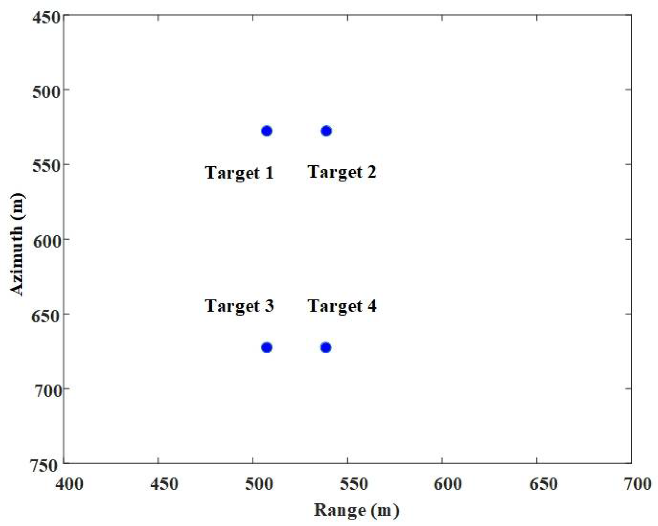
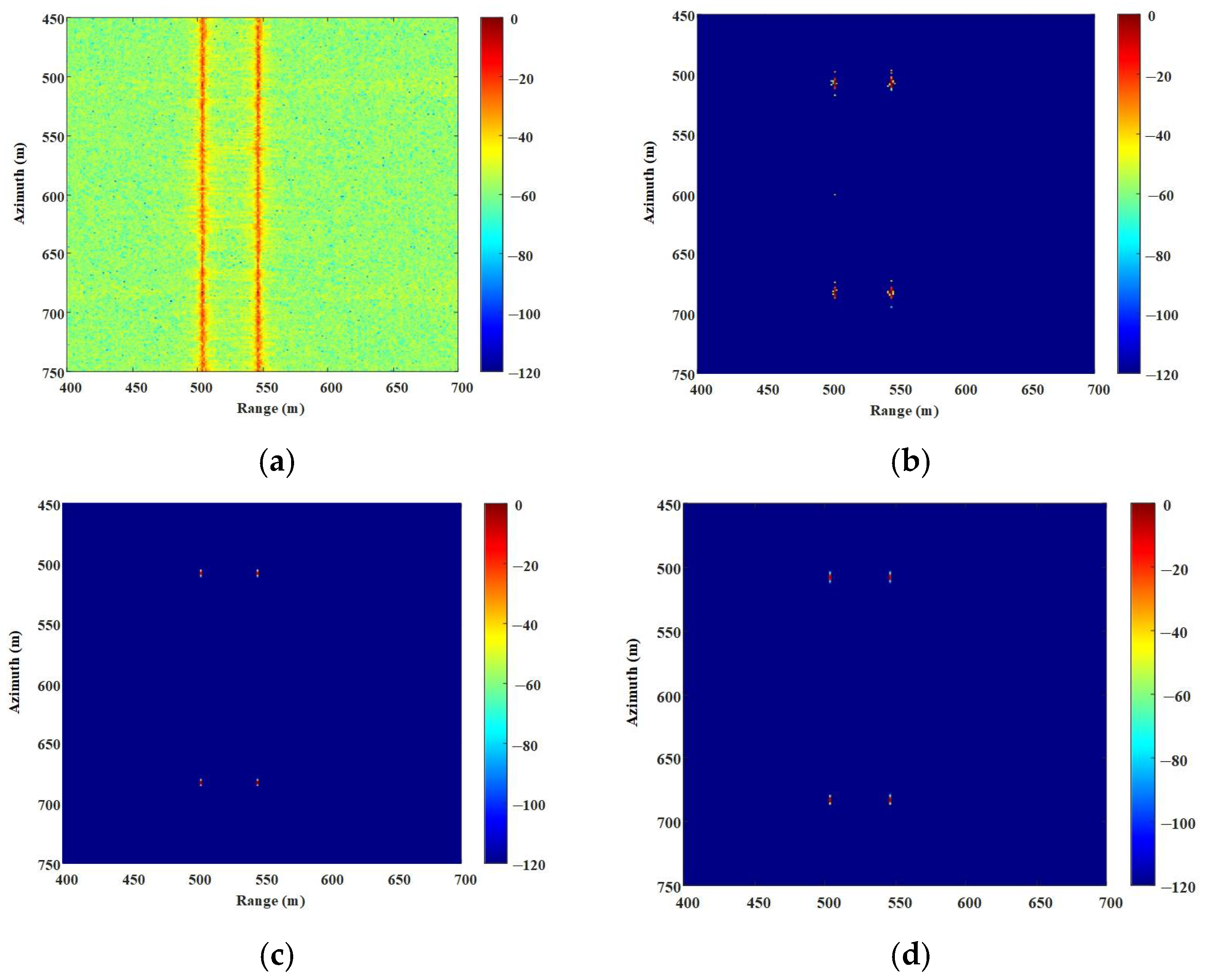
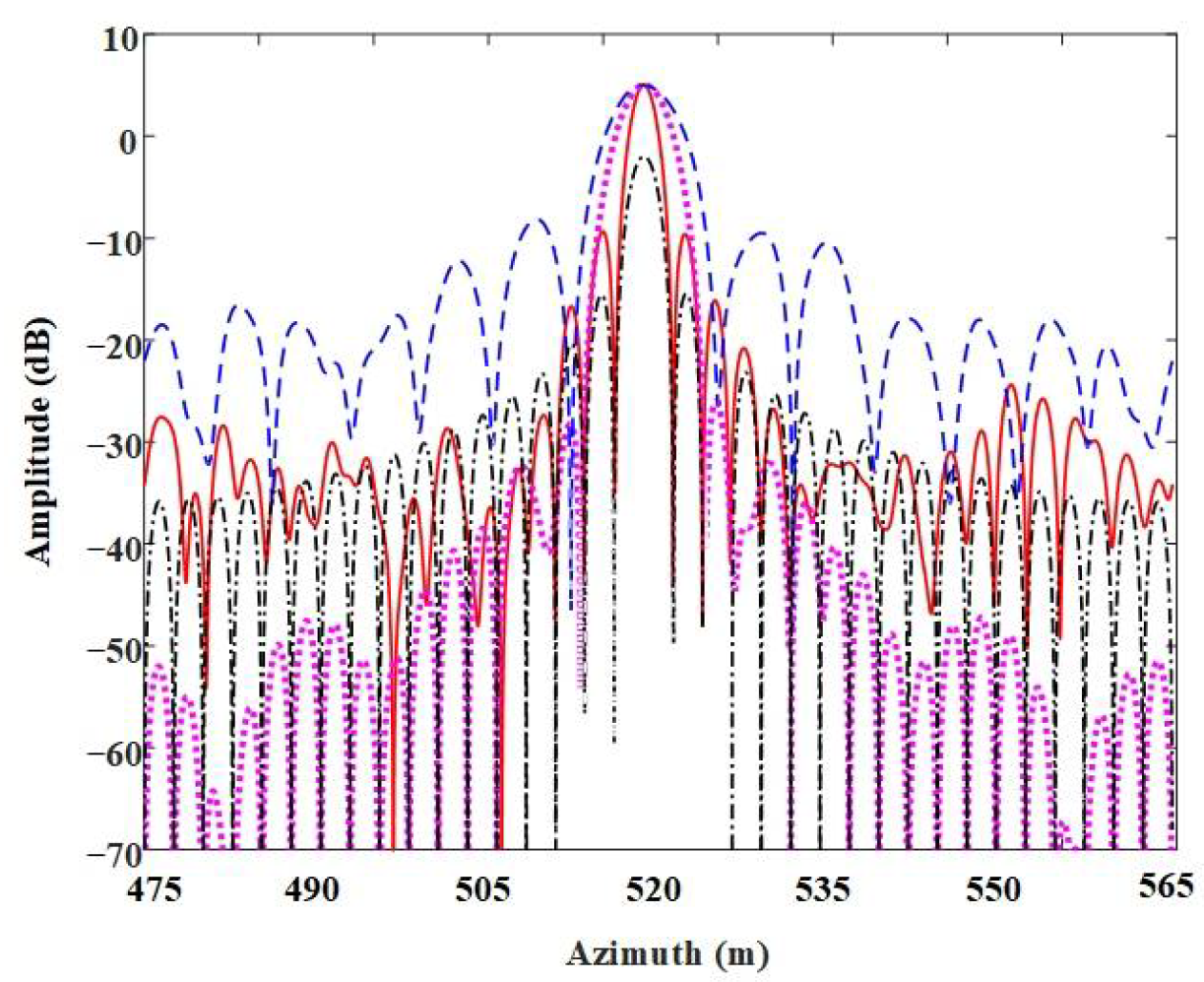
4.1. Point Target Simulation Experiment

In this study, the correlation imaging algorithm was used to conduct simulation analysis for point targets and regional targets when the airborne stripmap SAR system was operating in the side-looking imaging mode. The imaging algorithms used in this study included the chirp-scaling algorithm [27], the L1/2 regularization algorithm [28], the L1&TV algorithm [23], and the proposed algorithm. The imaging results and the performance of the four algorithms were analyzed. Table 2 provides the corresponding simulation configuration.
The point targets simulation layout is shown in Figure 3. The simulation parameters are presented in Table 2. The chirp-scaling algorithm, the L1/2 regularization algorithm, the L1&TV imaging algorithm, and the proposed algorithm were used to image the point targets, and the results are shown in Figure 4. In Figure 4, it can be seen that, although the traditional chirp-scaling algorithm could achieve basic point target reconstruction, its sidelobe suppression performance was insufficient, resulting in poor target focus. The L1/2 regularization algorithm and the L1&TV algorithm achieved better imaging results than the chirp-scaling algorithm in terms of sidelobe suppression, but the focusing effect still required further improvement. However, the proposed algorithm could significantly improve not only the focusing effect of the point targets but also the target energy concentration, ensuring better sparse reconstruction ability. Hence, compared to other methods, the proposed algorithm achieved significant improvements in the main performance-evaluation indicators, such as target focusing effect and sparse signal reconstruction accuracy.
To validate the effectiveness of the algorithms, we extracted an orientation slice of target 1 as an example. Comparatively, we analyzed the imaging performance of the four algorithms, and the results are shown in Figure 5. The evaluation results highlight the advantages of the proposed algorithm in providing optimal focus in the mainlobe region while significantly suppressing the sidelobe artifacts. While the conventional chirp scaling algorithm obtains a similar peak response in the mainlobe as the proposed algorithm, its sidelobe decay is relatively slow, which can significantly degrade the target’s azimuthal resolution and imaging quality. The L1/2 regularization algorithm improved the sidelobe characteristics by introducing sparse constraints, and its sidelobe level was lower than that of the chirp-scaling algorithm; however, the ideal suppression effect was not achieved. The L1&TV algorithm improved the imaging quality to a certain extent by introducing the TV regularization term constraint compared to the chirp-scaling algorithm; also, its mainlobe broadening was significantly reduced, but the sidelobe suppression effect required further improvement. Quantitative evaluation confirms that the proposed algorithm offers improved attenuation of sidelobe artifacts and sustains a narrow mainlobe width, surpassing the performance of existing methods. The results also proved that the proposed algorithm could effectively balance the relationship between the target focus and sidelobe suppression, thus improving the reconstruction accuracy.
In order to quantitatively evaluate the performance of the imaging algorithms, the point target slices under full sampling conditions were subjected to comparison using three key metrics: Peak Sidelobe Ratio (PSLR), Integrated Sidelobe Level Ratio (ISLR), and Impulse Response Width (IRW). These metrics were used to assess the performance of the four algorithms, with their corresponding values analyzed and compared in detail. The comparison results presented in Table 3 demonstrate that the proposed method outperformed all other algorithms in terms of imaging performance. Moreover, it significantly enhanced the resolution, which is particularly advantageous for imaging weak targets.
In order to comprehensively evaluate the performance of the proposed algorithm in terms of computational efficiency, Table 4 summarizes the corresponding theoretical computational complexity, actual reconstruction time-consuming and number of required iterations under normal sampling conditions for imaging scenes of M × N size, and compares them with the three typical reconstruction algorithms. All the experiments are performed in a unified hardware environment (processor: Intel Core i7-1065G7, 1.30 GHz, 8.0 GB RAM; Intel Corporation, Santa Clara, CA, USA).
From the comparison results in Table 4, it can be seen that, compared with other reconstruction algorithms, the proposed algorithm excels in terms of convergence speed and overall runtime. The proposed algorithm is able to complete the reconstruction task with fewer iterations while ensuring the imaging quality. Its efficient execution characteristics reflect the good design of the scheduling of the computational process, which effectively avoids redundant operations and repeated calculations.

4.2. Point Target Simulation Experiment Under Missing Data Condition

An experimental analysis was also performed on the point target imaging results of the four algorithms. In this experiment, data with 55% missing in the azimuth direction and a signal-to-noise ratio of −15 dB were used. By comparing the imaging results across the algorithms, performance variations under data loss conditions were assessed, which helped validate the noise resilience and robustness of the proposed method.
Figure 6 presents the point target imaging results of the four algorithms. It is evident that the chirp-scaling method exhibited a considerable decline in imaging quality under conditions of noise interference and sparse sampling. The L1/2 regularization algorithm and the L1&TV algorithm achieved clear imaging results, but they had obvious sidelobes, and their point target resolution was degraded. By contrast, the proposed algorithm could clearly image the point targets under the condition of noise and sparse sampling, achieving good focusing performance without obvious sidelobes.
Further, the showing of the four imaging algorithms was evaluated under the noise environment and data missing conditions. The imaging results of Target 1 were sliced, as shown in Figure 7, where it can be seen that, under these conditions, the proposed algorithm could still maintain a high degree of focus in the mainlobe area and effectively suppress the sidelobe. By contrast, the chirp-scaling algorithm could maintain a high target scattering intensity, but its sidelobe was significantly increased, showing a large oscillation throughout the observation domain. Compared with the chirp-scaling algorithm, the L1/2 regularization algorithm improved the anti-noise performance to a certain extent by introducing sparse constraints, but its sidelobe level was still higher than that of the proposed algorithm, and the integral sidelobe ratio performance needed to be improved.
Under conditions of significant noise interference and missing data, the proposed algorithm demonstrated superior performance by preserving a narrow mainlobe width while achieving better sidelobe suppression compared to existing methods. This highlights its robust anti-interference capability and effective target reconstruction performance in noisy environments.
To analyze the imaging quality quantitatively, the PSLR, ISLR, and IRW values of the point target column slices obtained by the four algorithms were compared, as shown in Table 5. The comparative analysis reveals that the proposed algorithm outperforms the benchmark methods in terms of imaging precision and overall reconstruction quality. In addition, the proposed algorithm could overcome the interference of noise and downsampling and had the best robustness performance among all algorithms.

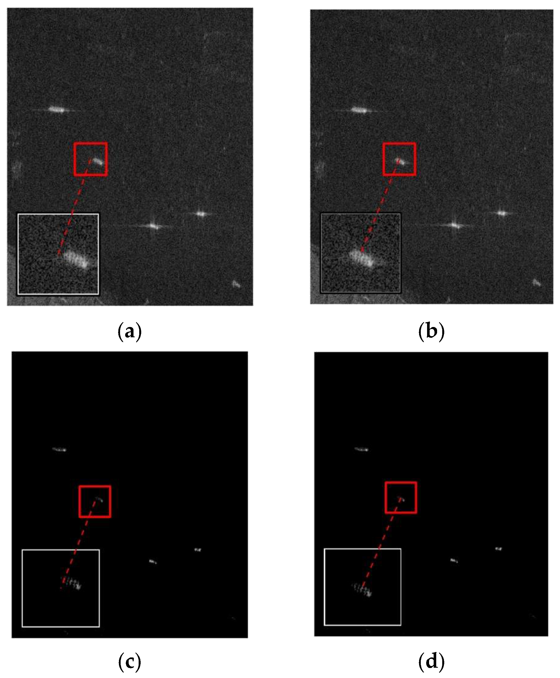
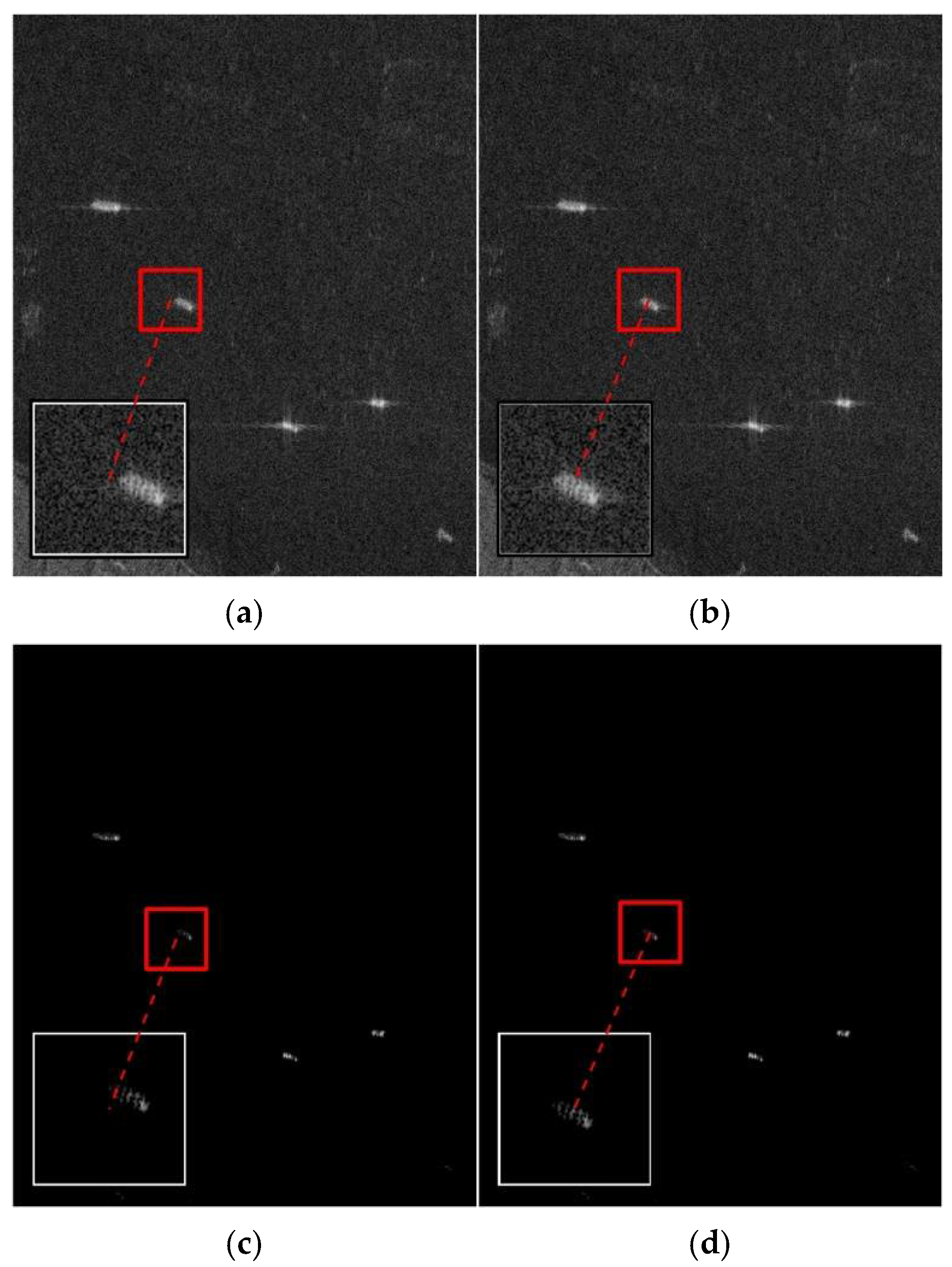
4.3. Imaging Experiment of Measured Data

In this experiment, the radar data from the RADARSAT-1 satellite were used to reconstruct images. The radar system parameters are shown in Table 6. To ensure an accurate image comparison analysis, four ships, marked by the red box in Figure 8, were selected as research objects. As illustrated in Figure 9, the reconstructed images obtained by the four evaluated methods demonstrate that all algorithms are capable of effectively recovering the structural features of the measured scene. However, compared with the other three algorithms, the algorithm proposed in this paper utilizes the sparse property of L₁ regularization to effectively suppress the scene noise and the sidelobes of the target, and filters out unwanted disturbances such as unstructured noise and clutter [29]; at the same time, it combines with the TV regularization to enhance the continuity of the image edges and structures, and suppresses the scattering noise and background clutter [24]. This regularization strategy has been validated in related fields and can significantly improve the robustness and noise reduction in reconstructed images. Hence, the proposed algorithm had obvious advantages in practical scene applications compared to the existing algorithms.
As shown in Figure 9 and Figure 10, and Table 7 and Table 8, the proposed algorithm performs well in the measured SAR data and maintains good imaging quality even in downsampling data. Compared with other algorithms, the proposed algorithm has significantly improved in core metrics of PSLR, ISLR, and IRW, showing good robustness and the ability to adapt to complex scenes. In addition, the proposed algorithm realizes an effective trade-off between sidelobe suppression and detail restoration, and significantly improves the image resolution and structural consistency, verifying its comprehensive advantages in target reconstruction.

4.4. Discussion

Based on the comparative analysis of simulation and measured data, the proposed algorithm demonstrates superior performance in terms of resolution, noise suppression, and robustness in imaging distributed targets compared to other methods. The L1 regularization effectively promotes a sparse representation of the image, while the TV regularization preserves edge clarity and structural continuity. The combination of these two regularization techniques significantly improves reconstruction quality under low signal-to-noise ratio conditions. The introduced approximate observation operator reduces computational complexity and memory overhead, enhancing the applicability of the method for SAR platforms with high real-time requirements.
Nevertheless, the method still has some limitations. Firstly, the reconstruction results are highly dependent on the proper setting of regularization parameters, which currently rely on empirical choices and lack an adaptive adjustment mechanism. Secondly, although the approximate observation model improves computational efficiency, it may introduce modeling errors in scenarios with complex scattering structures or dense target distributions, affecting image fidelity.
Future research will focus on developing more adaptive composite regularization frameworks to enhance the robustness of the method under incomplete data, complex interference, and motion error effects. Multi-regularization optimization mechanisms will be explored, incorporating motion compensation, interference suppression, and Doppler ambiguity correction to improve the practical performance of the algorithm on airborne SAR platforms.

5. Conclusions

In response to the issues of high data acquisition volume and low reconstruction efficiency in conventional SAR imaging, this paper presents a sparse reconstruction algorithm incorporating L1-TV regularization. Furthermore, a sparse SAR imaging framework is developed by integrating the chirp-scaling-based imaging operator with the echo simulation mechanism, enabling effective decoupling between azimuth and range dimensions. Moreover, the Newton accelerated iteration method is employed to accelerate the convergence speed of image reconstruction when determining the optimal solution. To validate the effectiveness of the proposed method, imaging experiments are conducted on both simulated and measured datasets, and the results are compared with those of three representative algorithms. The results indicate that the proposed algorithm can achieve fast and high-resolution reconstruction of a target under the conditions of azimuth data downsampling and noise interference and has a better imaging effect than similar existing algorithms.
Future research will focus on composite regularization methods for sparse SAR imaging. A novel optimization framework will be developed to enhance robustness and resolution under incomplete data, with attention to Doppler ambiguity, motion errors, and interference in airborne SAR. This approach aims to support high-fidelity imaging in complex environments and broaden applications in defense, disaster response, and geoscience.

Author Contributions

Conceptualization, Z.G. and H.M.; methodology, H.M.; software, H.M.; validation, Z.G. and H.M.; formal analysis, Z.G.; investigation, Z.G., H.M. and P.H.; resources, Z.G. and H.M.; data curation, Z.G. and H.M.; writing—original draft preparation, H.M.; writing—review and editing, Z.G. and P.H.; visualization, H.M.; supervision, W.X., W.T. and Z.W.; project administration, Z.G. and P.H.; funding acquisition, Z.G. and P.H. All authors have read and agreed to the published version of the manuscript.

Funding

This research was funded by National Natural Science Foundation of China under grant number 61761037, the Inner Mongolia Science and Technology Plan Project under grant number 2025SKYPT0044, the Basic Scientific Research Business Cost Project of Colleges directly under the Inner Mongolia under grant number ZTY2025034.

Data Availability Statement

The original contributions presented in this study are included in the article. Further inquiries can be directed to the corresponding author.

Conflicts of Interest

The authors declare no conflicts of interest.

References

  1. Cumming, I.G.; Wong, F.H. Digital processing of synthetic aperture radar data. Artech House 2005, 1, 108–110. [Google Scholar]
  2. Donoho, D.L. Compressed sensing. IEEE Trans. Inf. Theory 2006, 52, 1289–1306. [Google Scholar] [CrossRef]
  3. Herman, M.; Strohmer, T. Compressed sensing radar. In Proceedings of the 2008 IEEE International Conference on Acoustics, Speech and Signal Processing, Las Vegas, NV, USA, 31 March–4 April 2008; pp. 1509–1512. [Google Scholar]
  4. Liang, Y. Research on Time Series SAR Image Denoising Algorithm Based on Sparse Representation. Master’s Thesis, Chongqing Jiaotong University, Chongqing, China, 2024. [Google Scholar] [CrossRef]
  5. Chen, Y.; Jia, H.; Sun, Y.; Wen, J. High-Resolution Radar Range Profile Reconstruction Based on a Parametric Orthogonal Matching Pursuit Algorithm. J. Aerosp. Early Warn. Res. 2024, 38, 313–317. [Google Scholar]
  6. Hu, Y.; Gao, L.; Zhu, Y.; Sun, Z.; Guo, Z.; Ren, X. Sparse Diagnosis Method for Sudden Faults in Aero-Engine Gas Path Based on Improved Orthogonal Matching Pursuit. Propuls. Technol. 2024, in press. [Google Scholar]
  7. Hu, S.W.; Lin, G.X.; Hsieh, S.H.; Lu, C.S. Performance Analysis of Joint-Sparse Recovery from Multiple Measurement Vectors via Convex Optimization: Which Prior Information is Better? IEEE Access 2018, 6, 3739–3754. [Google Scholar] [CrossRef]
  8. Wu, G.; Luo, S. Adaptive fixed-point iterative shrinkage/thresholding algorithm for MR imaging reconstruction using compressed sensing. Magn. Reson. Imaging 2014, 32, 372–378. [Google Scholar] [CrossRef]
  9. Farhangkhah, N.; Samadi, S.; Khosravi, M.R.; Mohseni, R. Overcomplete pre-learned dictionary for incomplete data SAR imaging towards pervasive aerial and satellite vision. Wirel. Netw. 2024, 30, 3989–4001. [Google Scholar] [CrossRef]
  10. Du, W.; Hu, Y.; Sun, Y. Image Super-Resolution Reconstruction Method Based on Residual Dictionary Learning. J. Beijing Univ. Technol. 2017, 43, 43–48. [Google Scholar]
  11. Gao, Z.; Zhao, C.; Huang, P.; Xu, W.; Tan, W. Sparse Recovery STAP Algorithm Based on Adaptive Dictionary Correction. Signal Process. 2024, 40, 492–502. [Google Scholar] [CrossRef]
  12. Li, Y.; He, J.; Zhou, Y.; Hu, J.; Zhang, L. Sparse Denoising Method for Microseismic Signals in Mines Based on Adaptive Laplace Wavelet Dictionary. Energy Environ. Prot. 2024, 46, 69–76. [Google Scholar] [CrossRef]
  13. Luan, F.; Yang, F.; Cai, R.; Yang, C. Low-Sampling-Rate CT Reconstruction Based on Dual-Dictionary Adaptive Learning Algorithm. J. Northeast Univ. (Nat. Sci.) 2022, 43, 1709–1716. [Google Scholar]
  14. Wang, J.; Wang, Q.; Zheng, Y. Electrical Impedance Tomography Reconstruction Algorithm Based on L1 Regularization and Projection Method. In Proceedings of the 33rd Annual Conference of Tianjin Society of Biomedical Engineering, Tianjin, China, 10–11 June 2013; p. 1. [Google Scholar]
  15. Dong, X.; Zhang, Y. SAR Image Reconstruction from Undersampled Raw Data Using Maximum A Posteriori Estimation. IEEE J. Sel. Top. Appl. Earth Obs. Remote Sens. 2015, 8, 1651–1664. [Google Scholar] [CrossRef]
  16. Güven, H.E.; Güngör, A.; Çetin, M. An Augmented Lagrangian Method for Complex-Valued Compressed SAR Imaging. IEEE Trans. Comput. Imaging 2016, 2, 235–250. [Google Scholar] [CrossRef]
  17. Gao, Z.; Sun, S.; Huang, P.; Qi, Y.; Xu, W. Improved L1/2 Threshold Iterative High-Resolution SAR Imaging Algorithm. J. Radars 2023, 12, 1044–1055. [Google Scholar]
  18. Chen, M.; Mi, D.; He, P.; Deng, L.; Wei, B. A CT Reconstruction Algorithm Based on L1/2 Regularization. Comput. Math. Methods Med. 2014, 2014, 862910. [Google Scholar] [CrossRef]
  19. Gao, Z.; Li, X.; Huang, P.; Xu, W.; Tan, W. Sparse Microwave Imaging Algorithm Based on L1/2 Threshold Iteration and an Approximate Observation Operator. Electronics 2023, 12, 4574. [Google Scholar] [CrossRef]
  20. Zeng, J.; Xu, Z.; Zhang, B.; Hong, W.; Wu, Y. Accelerated L1/2 regularization based SAR imaging via BCR and reduced Newton skills. Signal Process. 2013, 93, 1831–1844. [Google Scholar] [CrossRef]
  21. Zhao, J.; Jiang, Z.; Liu, B.; Zhang, L. Moving Target Detection Based on L1/2-TV Regularized RPCA. Comput. Simul. 2024, 41, 258–263, 428. [Google Scholar]
  22. Liu, Z.; Xu, Y.; Dong, F. L1-L2 Spatial Adaptive Regularization Method for Electrical Tomography. In Proceedings of the 2019 Chinese Control Conference (CCC), Guangzhou, China, 27–30 July 2019; pp. 3346–3351. [Google Scholar]
  23. Liu, M.; Xu, Z.; Chen, T.; Zhang, B.; Wu, Y. Low-Oversampling Staggered SAR Imaging Method Based on L1&TV Regularization. Syst. Eng. Electron. Technol. 2023, 45, 2718–2726.24. [Google Scholar]
  24. Li, M.; Cai, G.; Bi, S.; Zhang, X. Improved TV Image Denoising over Inverse Gradient. Symmetry 2023, 15, 678. [Google Scholar] [CrossRef]
  25. Fang, J.; Xu, Z.; Zhang, B.; Hong, W.; Wu, Y. Fast Compressed Sensing SAR Imaging Based on Approximated Observation. IEEE J. Sel. Top. Appl. Earth Obs. Remote Sens. 2014, 7, 352–363. [Google Scholar] [CrossRef]
  26. Liu, M.; Pan, J.; Zhu, J.; Chen, Z.; Zhang, B.; Wu, Y. A Sparse SAR Imaging Method for Low-Oversampled Staggered Mode via Compound Regularization. Remote Sens. 2024, 16, 1459. [Google Scholar] [CrossRef]
  27. Raney, R.K.; Runge, H.; Bamler, R.; Cumming, I.G.; Wong, F.H. Precision SAR processing using chirp scaling. IEEE Trans. Geosci. Remote Sens. 1994, 32, 786–799. [Google Scholar] [CrossRef]
  28. Xu, Z.; Chang, X.; Xu, F.; Zhang, H. L1/2 Regularization: A Thresholding Representation Theory and a Fast Solver. IEEE Trans. Neural Netw. Learn. Syst. 2012, 23, 1013–1027. [Google Scholar] [CrossRef]
  29. Duan, L.; Sun, S.; Zhang, J.; Xu, Z. Deblurring Turbulent Images via Maximizing L1 Regularization. Symmetry 2021, 13, 1414. [Google Scholar] [CrossRef]
Figure 1. Side-looking radar imaging relationship diagram.
Electronics 14 02508 g001
Figure 2. Flowchart of sparse SAR imaging algorithm based on L1-TV regularization.
Electronics 14 02508 g002
Figure 3. Point target simulation layout.
Electronics 14 02508 g003
Figure 4. Point target imaging results of different algorithms: (a) the chirp-scaling algorithm; (b) the L1/2 regularization algorithm; (c) the L1&TV algorithm; (d) the proposed algorithm.
Electronics 14 02508 g004
Figure 5. Point target slice comparison results: —, proposed algorithm; -.-.-.-., L1/2 regularization algorithm; ———, chirp-scaling algorithm; ….., L1&TV algorithm.
Electronics 14 02508 g005
Figure 6. Point target imaging results of the four algorithms under the condition of missing data: (a) the chirp-scaling algorithm; (b) the L1/2 regularization algorithm; (c) the L1&TV algorithm; (d) the proposed algorithm.
Electronics 14 02508 g006
Figure 7. Point target slices in the case of downsampling and noise: —, proposed algorithm; -.-.-.-., L1/2 regularization algorithm; ———, chirp-scaling algorithm; ….., L1&TV algorithm.
Electronics 14 02508 g007
Figure 8. RADARSAT-1 measured data imaging results.
Electronics 14 02508 g008
Figure 9. Imaging results of the RADARSAT-1 partial measured data obtained by the four algorithms: (a) the chirp-scaling algorithm; (b) the L1/2 regularization algorithm; (c) the L1&TV algorithm; (d) the proposed algorithm.
Electronics 14 02508 g009
Figure 10. Imaging results of the RADARSAT-1 (azimuthally missing 55%) portion of the measurements obtained by four algorithms: (a) chirp scaling algorithm; (b) L1/2 regularization algorithm; (c) L1&TV algorithm; (d) the proposed algorithm.
Electronics 14 02508 g010
Table 1. Sparse SAR imaging algorithm based on the L1-TV regularization method.
Input:Two-Dimensional Echo Data Y, Iteration Step Parameter δ, The Maximum Iteration Number tmax, Error Parameter ε, Image Size N, Noise Variance σ, Lagrange Multipliers ξ1 and ξ2.
Initialization: X 0 = 0 , k = 0 , d p = ( 0 , 0 ) , z 1 ( 0 ) = 0 , z 2 ( 0 ) = 0 , v z 1 ( 0 ) = 0 , v z 2 ( 0 ) = 0
Iteration: w h i l e   t < t m a x   &   &   R e s > ε
1. X ( k + 1 ) = [ L G I + ξ 1 + ξ 2 I ] 1 [ L ( B * Y ) + ξ 1 z 1 ( k ) + ξ 2 z 2 ( k ) ]
2. z 1 Γ ( z 1 ( k ) ~ ) = λ 1 ( k ) s i g n ( z 1 ( k ) ) + 2 ξ 1 ( z 1 ( k ) X ( k ) ) z 2 Γ ( z 2 ( k ) ~ ) = λ 2 ( k ) s i g n ( z 2 ( k ) ) + 2 ξ 2 ( z 2 ( k ) X ( k ) )
3. v z 1 ( k + 1 ) = β v z 1 ( k ) z 1 Γ ( z 1 ( k ) ~ ) ; v z 2 ( k + 1 ) = β v z 2 ( k ) z 2 Γ ( z 2 ( k ) ~ )
4. z 1 ( k + 1 ) = z 1 ( k ) + β v z 1 ( k ) ; z 2 ( k + 1 ) = z 2 ( k ) + β v z 2 ( k )
5. λ 1 ( k + 1 ) = 2 ξ 1 s i g n ( X ( k + 1 ) z 1 ( k + 1 ) )
6. d p i , j ( k + 1 ) = d p i , j ( k ) + δ ( ( d i v d p ( k ) | X ( k + 1 ) | / λ T V ) ) i , j m a x { | d p i , j ( k ) + δ ( ( d i v d p ( k ) | X ( k + 1 ) | / λ T V ) ) i , j | , 1 }
7. λ 2 ( k + 1 ) = X ( k + 1 ) 2 ξ 2 z 2 ( k + 1 ) d i v ( d p ( k + 1 ) )
8. λ T V = λ 2 ( k + 1 ) 2 ξ 2
9. R e s = X ( k + 1 ) X ( k ) 2 / X ( k ) 2
10. k = k + 1
End while
Output:Image sparse reconstruction X ( k + 1 )
Table 2. Experimental configuration for L1-TV enhanced sparse SAR imaging.
ParameterNumerical Value
Effective speed of radar platform (m/s)150
Scene center slant distance (km)10
Doppler bandwidth (MHz)7.967
Distance sampling rate (MHz)60
Azimuth sampling rate (Hz)200
Operating frequency (GHz)5.3
Table 3. Performance of different imaging algorithms obtained using full sampling.
AlgorithmPSLR (dB)ISLR (dB)IRW (m)
Chirp-scaling algorithm−13.2764−10.17941.6641
L1/2 regularization algorithm−13.1921−10.26221.6503
L1&TV algorithm−25.9566−18.89731.6592
Proposed algorithm−26.3846−23.14821.6979
Table 4. Evaluation of execution time, computational complexity, and iteration count.
AlgorithmTime
Consumption(s)
Computational ComplexityNumber
of Iterations
Chirp-scaling algorithm0.915O(MN.log(MN))1
L1/2 regularization algorithm29.134O(T.log(MN)2)300
L1&TV algorithm21.919O(T.log(MN)2)10
Proposed algorithm8.913O(T. log(MN)2)4
Table 5. Performance of different imaging algorithms in the case of downsampling and noise.
AlgorithmPSLR (dB)ISLR (dB)IRW (m)
Chirp-scaling algorithm−12.9965−9.48121.4323
L1/2 regularization algorithm−11.2364−9.98811.4670
L1&TV algorithm−22.2001−16.20281.5702
Proposed algorithm−22.6146−18.89731.5065
Table 6. Main system parameters of the RADARSAT-1 stripe mode.
ParameterNumerical Value
Operating frequency (GHz)5.3
Emission pulse width (MHz)30.111
Radar emission wavelength (m)5.6 × 10⁻⁶
Radar effective rate (m/s)7062
Distance frequency modulation (MHz/s)73,150
Azimuth frequency modulation (Hz/s)1755
Distance sampling rate (MHz)3.2317
Pulse repetition frequency (Hz)1257
Table 7. Performance of different imaging algorithms on fully sampled actual measurement data.
AlgorithmPSLR (dB)ISLR (dB)IRW (m)
Chirp-scaling algorithm−10.08−11.032.28
L1/2 regularization algorithm−10.91−11.242.26
L1&TV algorithm−17.84−18.001.89
Proposed algorithm−18.55−18.421.86
Table 8. Performance of different imaging algorithms on actual measurement data under downsampling conditions.
AlgorithmPSLR (dB)ISLR (dB)IRW (m)
Chirp-scaling algorithm−0.22−11.0016.85
L1/2 regularization algorithm−1.29−9.709.28
L1&TV algorithm−10.33−11.552.39
Proposed algorithm−11.24−18.552.15
Disclaimer/Publisher’s Note: The statements, opinions and data contained in all publications are solely those of the individual author(s) and contributor(s) and not of MDPI and/or the editor(s). MDPI and/or the editor(s) disclaim responsibility for any injury to people or property resulting from any ideas, methods, instructions or products referred to in the content.

