1. Introduction
With the development of modern electronic countermeasure (ECM) technologies and computing power, radar jamming techniques have become increasingly complex and diverse [
1,
2]. Consequently, radar anti-jamming decision-making plays an increasingly important role in modern radar applications [
3]. In 2006, Haykin introduced the concept of cognitive radar [
4], and foresightedly highlighted the application prospects of Bellman’s Dynamic Programming Equation in adaptive algorithms for radar signal processing research. In order to address the problems of intelligent decision-making in radar anti-jamming, existing research analyzes the problem from the perspectives of game theory and reinforcement learning (RL).
Generally, the interaction between radar systems and jammers can be modeled as a two-player zero-sum (TPZS) game [
5,
6], where both sides attempt to select optimal strategies to maximize their own gains and maximize losses for the opponent [
7]. The strategy that brings both sides to a steady state is referred to as the Nash Equilibrium (NE) [
8] strategy. However, in complex jamming environments, the model faces a large state and action space, and the information obtained by the model is usually limited. Strategy optimization based solely on game theory struggles to achieve absolute rationality, thus requiring strategies to be gradually improved through continuous learning steps.
As a branch of machine learning (ML), RL primarily addresses exploring and learning optimal strategies. RL, which shows great application potential, has achieved significant progress in energy management [
9], robotic control [
10], communication network optimization [
11], and in many other fields [
12,
13,
14]. RL aims to achieve a stated goal by continuously learning and adapting its strategy in a dynamic environment, and learning how to take actions to maximize rewards. Driven by the wave of intelligent development, the introduction of the RL algorithm provides radar with an adaptive and dynamic anti-jamming strategy optimization method, which can effectively deal with the decision-making difficulties brought about by the diversity of jamming signals. As a typical RL algorithm,
Q-learning uses a value function approximation represented by a
Q-value table.
Q-learning provides an effective solution for low-dimensional decision-making problems, but as the state and action spaces grow, the size of the
Q-value table increases exponentially, which not only slows down the computation speed but also severely increases the cost of the decision-making system [
15].
Compared to table-based value approximation, the deep Q-network (DQN) employs neural networks to approximate value functions and uses experience replay to reduce temporal correlation among data samples. Experiments have shown that DQN substantially outperforms Q-learning in high-dimensional state and action spaces. With the application of DQN, the radar anti-jamming strategy model can accommodate more anti-jamming actions to cope with the complex jamming environment.
However, there are still drawbacks to DQN. Since action evaluation and selection are performed by the same network, DQN tends to overestimate action values to varying degrees. And this overestimation is magnified, step by step, during the training process, which is called ‘bootstrapping’, causing local optima and convergence difficulties. To address these issues, the double deep
Q-network (DDQN) employs separate evaluation and target networks to mitigate action value overestimation. At the same time, DDQN improves the calculation of the target
Q-value to further mitigate overestimation compared to DQN. Up to this point, DDQN has made improvements to address the overestimation of the value function, but in more complex environments, the performance of DDQN still faces challenges. First, DDQN relies on the
-greedy exploration strategy, which tends to select random rather than optimal actions to some extent. The usual approach to solving the above problem is to gradually decrease
with the number of training steps. But this solution relies heavily on the initial value of
and the rate of descent; inappropriate values will lead to local optima and a slow convergence rate. Second, traditional experience replay collects experiences with equal probability, which ignores differences between experiences. In a dynamic environment, the speed of model convergence will be affected. Lastly, hyperparameters such as learning rate, discount factor, and target network update frequency significantly impact DDQN convergence speed and generalization ability [
16], and fixed hyperparameter settings are inadequate for complex tasks. Regarding the above issues, some models optimize the DDQN network structure [
17,
18,
19,
20] by employing a dueling double deep
Q-network [
21], which reconstructs the
Q-value as a state-value function and an action advantage value, allowing the agent to learn the state-value more frequently and accurately. Other models choose to improve experience replay [
22,
23], adopting prioritized experience replay (PER) [
24] to preferentially replay high-value experiences, thereby improving data utilization and learning speed.
In existing research, radar anti-jamming decision-making methods mainly focus on three aspects, namely, overall anti-jamming strategy optimization, anti-jamming waveform strategy optimization, and frequency selection strategy optimization. Ref. [
19] proposed a cognitive radar anti-jamming strategy generation algorithm based on a dueling double deep
Q-network, which shows that the dueling double deep
Q-network generates a more effective anti-jamming strategy than DQN. Ref. [
20] generates the anti-jamming waveform strategy for airborne radars based on the dueling double deep
Q-network as well as PER, and uses an iterative transformation method (ITM) to generate the time domain signals of the optimal waveform strategy. The simulation results demonstrate the improved effect of the dueling double deep
Q-network and PER. Yet, these improvements still exhibit slow convergence and potential local optima in complex jamming environments. Ref. [
25] established both radar and jammer as agents, and found the optimal power allocation strategy for the radar by using the multi-agent deep deterministic policy gradient (MADDPG) algorithm based on multi-agent reinforcement learning. Ref. [
26] presented an NE strategy for radar-jammer competitions involving dynamic jamming power allocation by utilizing an end-to-end deep reinforcement learning (DRL) algorithm, considering that the competition between the radar and the jammer involves imperfect information. Additionally, Ref. [
27] proposed a slope-varying linear frequency modulation (SV-LFM) signal strategy generation method based on DQN, enabling radar systems to learn optimal anti-jamming strategies without prior information.
Moreover, compared to other types of radar systems, phased-array radars offer greater flexibility in selecting the positions and number of auxiliary antennas. This capability provides higher adaptability in dynamically changing jamming environments. Therefore, to address the above problems, this paper makes comprehensive improvements to the aforementioned methods and proposes a phased-array radar anti-jamming decision-making approach with high accuracy in environments where multiple types of jamming coexist. A noisy network constructed using factorized Gaussian noise [
28] is incorporated to dynamically adjust action selection randomness during training, thereby enhancing exploration efficiency. Moreover, n-step temporal difference learning [
29] is employed to update the
Q-value using multi-step returns, accelerating reward propagation. The above improvements are combined with a dueling network and DDQN to achieve comprehensive performance enhancement. Additionally, as an improvement of double-depth priority experience replay (DDPER) [
30], this paper proposes variable double-depth priority experience replay (VDDPER), which refines experience learning mechanisms by dynamically adjusting the proportion of deep and shallow experiences utilized during training, further accelerating model convergence. The main contributions of this work are as follows:
To improve the reward convergence speed and decision accuracy, a multi-aspect improved deep Q-network (MAI-DQN) algorithm for phased-array radar anti-jamming decision-making is proposed. In the MAI-DQN, the noisy network based on factorized Gaussian noise is used to improve the exploration policy. And n-step learning and DDQN are used to update the temporal difference target value, thereby improving the reward propagation of long sequence tasks. In addition, the dueling network is used to decompose the Q-value into two parts, thereby introducing the concept of advantage and further improving the network structure. Moreover, target soft update, variable learning rate, and gradient clipping are used to further improve the training effect.
To enhance the utilization of experience replay across all experiences in the early stages of training and emphasize high-value experiences in the later stages of training, the VDDPER mechanism is proposed as an improvement over DDPER. VDDPER dynamically adjusts the sample sizes for different values of experience to direct the model’s attention toward experiences of different values during training.
To accurately characterize jamming states in complex environments and enable optimal anti-jamming measures, a novel and effective design of the state space, action space, and reward function—combining data-level and signal-level benefits—is proposed and shown to achieve rapid convergence during training.
The remainder of this paper is organized as follows: In
Section 2, the phased-array radar echo signal model, array configuration, and interactive system model for the radar and the jammer competition are introduced. In
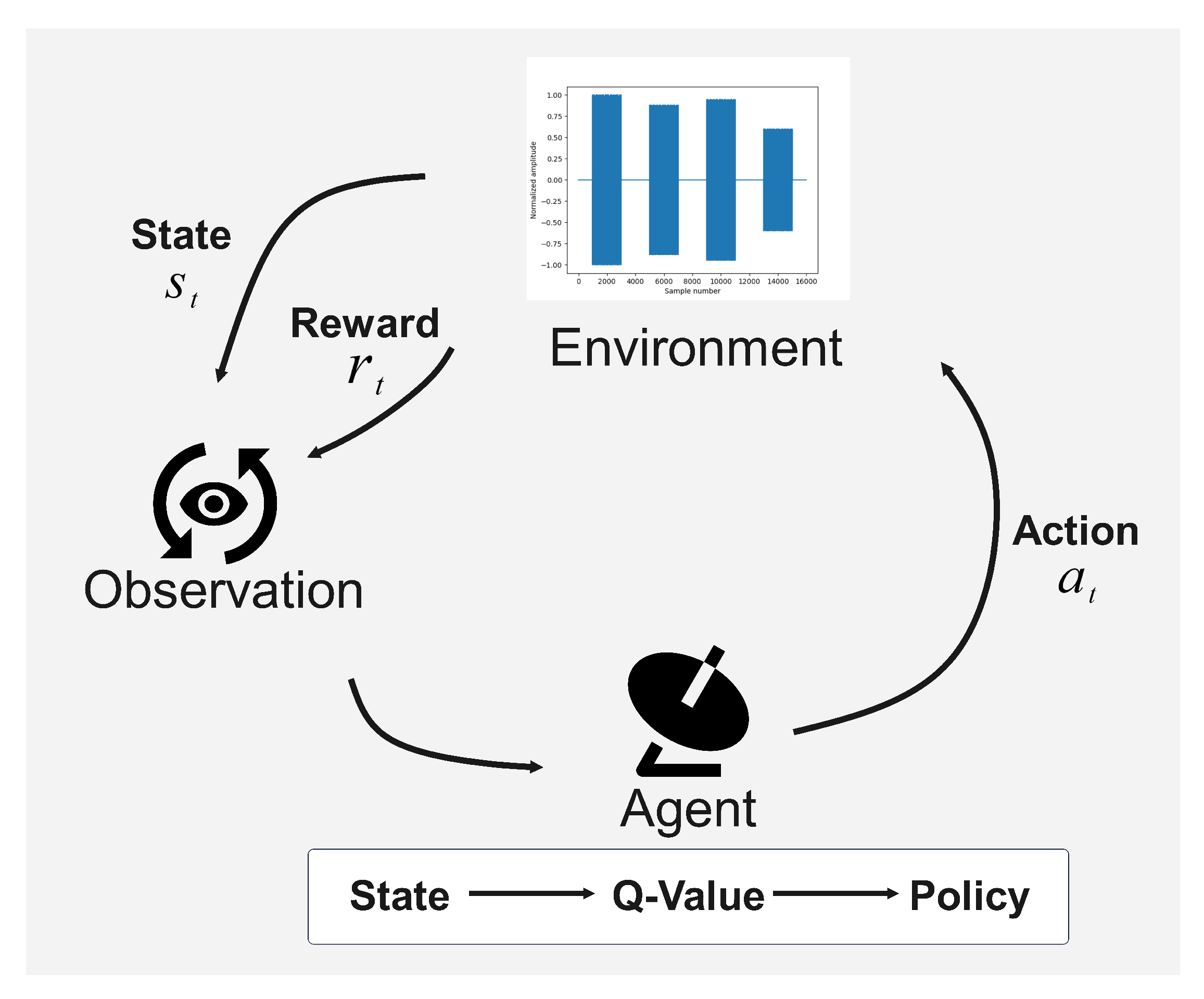
Section 3, the RL decision-making process and the basic concepts with DQN are analyzed and described.
Section 4 presents the implementation of MAI-DQN in phased-array radar anti-jamming decision-making and outlines its improvements in detail.
Section 5 describes the experimental setup for several RL algorithms and MAI-DQN, followed by a comparison and analysis of the experimental results. Finally, the conclusion and some future works are shown in
Section 6.
2. System Model
In this section, we introduce the basic concept of phased-array radar and analyze the echo signal model. Then, we introduce and analyze the environmental interaction model between the phased-array radar and the jammer.
As a kind of array radar, phased-array radar controls the beam direction by adjusting the phase of individual antenna elements within the array, allowing for rapid scanning, multi-target tracking, and enhanced anti-jamming capabilities. Essentially, it represents a signal processing approach implemented in the analog domain using radio frequency (RF) components and feed networks. This paper focuses on a monostatic uniform linear array (ULA) phased-array radar. Therefore, an accurate echo model is established. When employing a linear frequency modulation (LFM) signal, the single-target echo signal model for an
M-element phased-array radar can be expressed as follows:
where
represents the signal envelope with a pulse width of
T;
denotes the carrier frequency;
represents the target propagation delay;
k denotes the signal chirp rate;
denotes the target Doppler shift; and
represents the initial phase of the echo signal. Additionally,
denotes the signal steering vector:
where
d denotes the inter-element spacing of the antenna array, and
denotes the radar wavelength. To avoid grating lobes, most ULA-configured phased-array radars set the element spacing to
.
accounts for the influence of the target’s radar cross-section (RCS). In this paper, a log-normal distribution RCS fluctuation model is employed to simulate large naval targets, with the probability density function defined as follows:
where
represents the median RCS value, and
denotes the ratio between the average and median RCS values.
Moreover, this paper employs frequency agility (FA) and cover pulse techniques as active anti-jamming strategies. When the radar adopts an FA waveform, the single-target echo signal model can be expressed as follows:
where
represents the carrier frequency of the
m-th pulse,
,
controls the frequency hopping of the
m-th pulse, and
denotes the minimum frequency hopping interval. When the radar employs a cover pulse waveform, it simultaneously transmits multiple carrier frequencies to deceive jammers into intercepting incorrect frequency points. Assuming that the real signal carrier frequency is
this time, the cover pulse waveform echo signal model will not be repeated here.
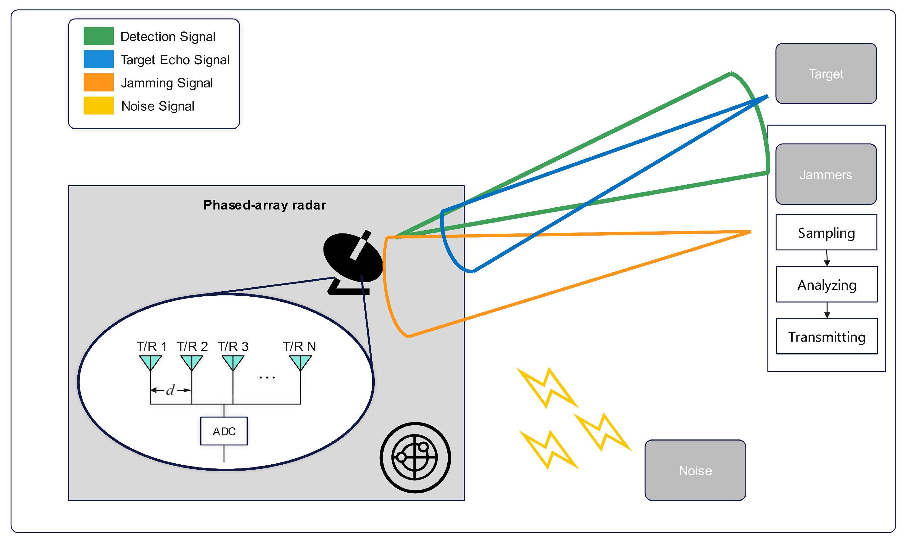
As shown in
Figure 1, when operating in search mode, the radar transmits signals to scan the target region. Part of the signal is reflected by the target and is received as an echo by the radar, while part of the signal is intercepted by the jammer. Using digital radio frequency memory (DRFM) technology, the jammer samples and stores the intercepted signal at high speed. After analyzing the signal characteristics, the jammer decides whether to transmit suppression or deception jamming signals to interfere with the radar in the time, frequency, or energy domains. At the same time, noise signals represented by Gaussian white noise are also received by the radar due to the presence of thermal noise from the electronics in the radar, as well as atmospheric noise and other effects.
Regarding jamming, this paper investigates various types of jamming signals [
31,
32,
33,
34], including dense false target jamming, sweep jamming, coherent slice forwarding jamming, and spot jamming, as shown in
Figure 2, alongside the target echo and noise signals. Due to the presence of multiple jammers, the above types of jamming may co-exist, and based on the jamming direction, the above types of jamming can be categorized as mainlobe, sidelobe, or combined mainlobe–sidelobe jamming. In addition, random phase perturbations are introduced across all types of jamming to simulate potential uncertainties such as the phase noise from the jammer, phase disturbance strategies, and multipath effects.
Regarding anti-jamming measures and anti-jamming strategies, this paper incorporates frequency agility, cover pulses, the sidelobe canceller (SLC) algorithm, and sidelobe blanking (SLB) as anti-jamming measures. During the game process with the jammer, the model iteratively explores and generates the most effective combination of anti-jamming measures, leading to the derivation of the optimal anti-jamming strategy.
Since electromagnetic waves in free space satisfy the principle of linear superposition, and the target echo signal, jamming signal, and noise are independent, these three signals are generally additive. Under such conditions, the radar’s received signal model can be expressed as follows:
where
denotes the target echo signal,
represents the jamming signal under one or more jamming, and
accounts for noise. The amplitude factor of the target echo is given by the following:
where
represents the signal-to-noise ratio,
denotes the standard deviation of Gaussian white noise, and the amplitude factor of the jamming signal is as follows:
where
represents the jamming-to-noise ratio.
After constructing the signal model, additional metrics beyond
and
are required to comprehensively evaluate the signal quality before and after anti-jamming measures, thereby accurately reflecting the effectiveness of anti-jamming strategies. The first metric is the interference suppression ratio, reflecting the effectiveness of anti-jamming techniques in suppressing jamming signal energy. The interference suppression ratio
can be expressed as follows:
where
denotes the energy of the jamming signal before suppression, and
represents the remaining energy of the jamming signal after suppression.
Another evaluation metric is the radar target detection result after pulse compression and cell-averaging constant false alarm rate (CA-CFAR) processing, which assesses the effectiveness of anti-jamming measures in filtering out false targets. As a classical constant false alarm rate method, CA-CFAR estimates the detection threshold based on a set of neighboring background noise cells and compares it with the signal level in the target cell to determine the presence of a target. Generally, the CA-CFAR detection threshold is given by the following:
where
represents the threshold scaling factor,
denotes the estimated reference noise level,
denotes the predetermined false alarm probability,
denotes the number of reference cells, and
denotes the amplitude of the echo signal in the
i-th reference cell.
Moreover, a set of data-level evaluation metrics is designed within the reward function to assess the effectiveness of anti-jamming measures in the frequency domain.
4. MAI-DQN for Anti-Jamming Decision-Making
The traditional DQN algorithm cannot achieve fast reward convergence and an accurate anti-jamming strategy in complex jamming environments. For this reason, the MAI-DQN is proposed.
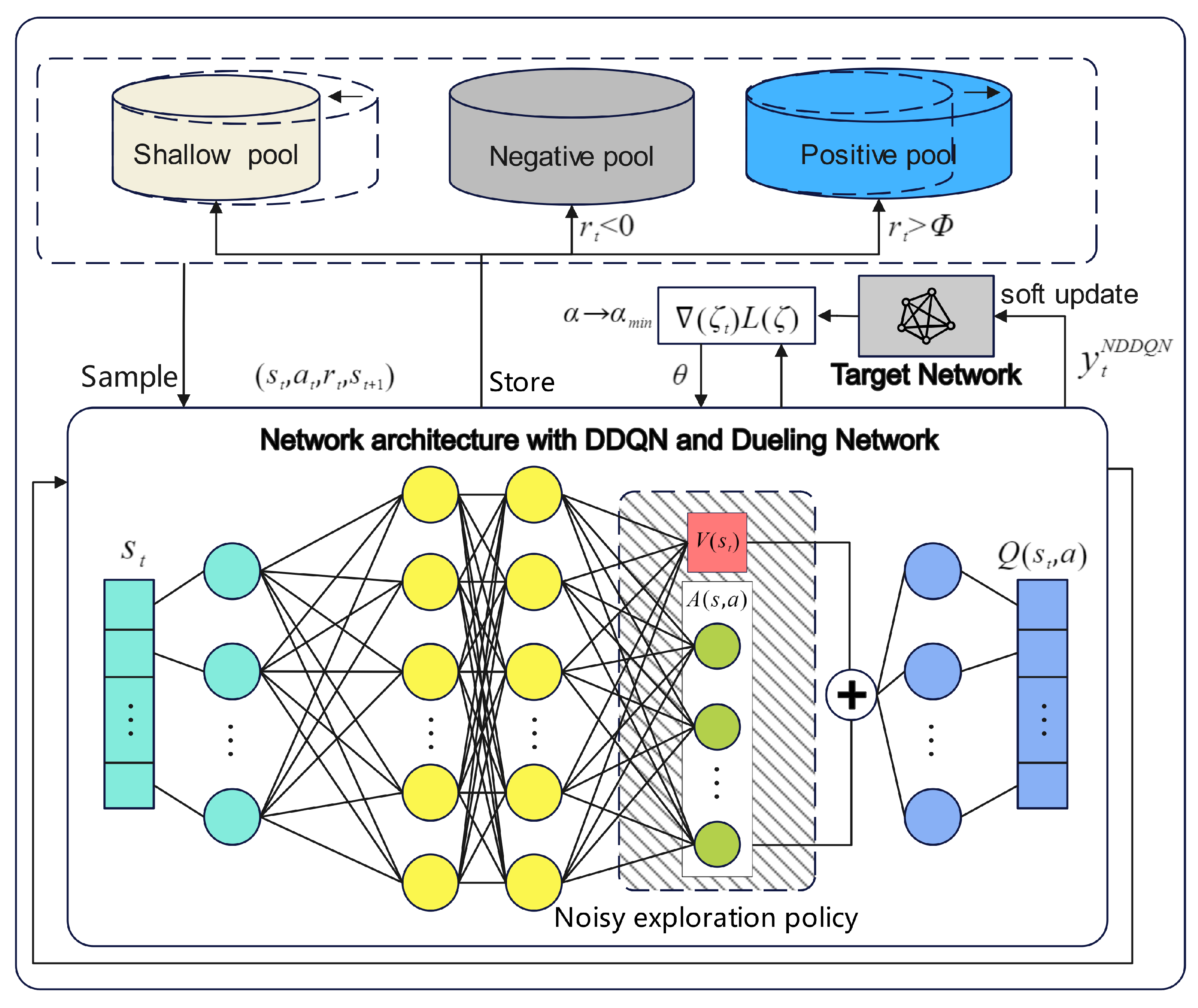
In this section, the improvements made to the algorithms of this paper for DQN are detailed in terms of network architecture, exploration strategy, and training methods. Then, the state and action spaces of the phased-array radar anti-jamming decision-making model are introduced in detail, and a detailed solution for the phased-array radar anti-jamming strategy based on MAI-DQN is given. As shown in
Figure 4, in terms of network architecture, the current signal state
of the phased-array radar is input into the network architecture enhanced with DDQN and a dueling network. In terms of exploration policy, the action is selected through the noisy network, and then the TD error values for training are obtained. In terms of training methods, the network parameters are updated using the TD error generated by the n-step TD method. The variable learning rate, soft update, and gradient clipping are used by the model to improve training results. Finally, the
Q-value corresponding to the current anti-jamming action is output. In this process, VDDPER stores the current experience in three separate pools based on the reward magnitude for efficient experience replay and adjusts the sample size according to the value of each experience.
4.1. Network Architecture
4.1.1. Double Deep Q-Network
In the network architecture, the MAI-DQN algorithm incorporates a double deep
Q-network (DDQN) to further mitigate the overestimation issue observed in DQN. When calculating the one-step TD target value in DDQN, the action corresponding to the maximum
Q-value is initially selected using the evaluation network:
then, the improved one-step TD target value method can be expressed as follows:
4.1.2. Dueling Network
MAI-DQN further improves the learning efficiency and generalization capability of DQN by introducing a dueling network structure. In the DQN neural network architecture, the fully connected layers directly connect to the output layer, producing the
Q-values corresponding to each action for the current state after training. In contrast, the dueling network introduces two separate branches following the linear layers, forming two evaluation modules—one evaluates the state value
, referred to as the state-value network, and another predicts the advantage of each action
, known as the advantage network. This structure ensures that the assessment of the state does not entirely depend on the value of actions, enabling the model to better converge when actions have a limited impact on state value. In the dueling network, the
Q-value output can be represented as follows:
where
and
are parameters corresponding to the advantage network and the state-value network, respectively, used for function optimization.
However, because the above equation overly emphasizes the summed result of
and
, it cannot yield accurate and fixed values of
and
when given a certain
Q-value, potentially leading to unstable or non-convergent training. Therefore, the following improvement is proposed:
where
.
According to the improvement of the above equation, both and yield similar solutions for a given Q-value.
4.2. Exploration Policy
As previously mentioned, the traditional DQN employs an -greedy exploration policy. However, both the parameter and its decay rate require manual configuration. Optimal exploration strategies may vary across different scenarios or different parameter settings within the same scenario, and manually tuning the parameters of the exploration policy may cause slower convergence or suboptimal performance. Additionally, in certain states, some actions may clearly be suboptimal, yet the -greedy policy still randomly selects these actions with probability and reduces exploration efficiency.
To address this issue, this paper introduces a noisy network to enhance the exploration policy. The noisy network incorporates learnable stochastic noise into the weights of the neural network, enabling the agent to automatically adjust the degree of exploration according to different states. For a neural network, a linear network layer with input
p and output
q can be represented by the following equation:
where
,
,
represents the weight matrix, and
denotes the bias vector. Both
and
b are learnable parameters in the network. When noise is introduced, the equation is as follows:
where
,
,
, and
. The symbol ⊙ denotes the Hadamard product, and
,
are random noise variables.
In the noisy network, parameters
,
,
, and
are learned and updated through gradient descent, whereas the noise variables
and
are generated using factorized Gaussian noise. Specifically,
p values are sampled independently from a Gaussian distribution to obtain
firstly, and subsequently,
q values are sampled independently from a Gaussian distribution to obtain
. The noise variable
is then calculated as follows:
where
, similarly,
can be expressed as follows:
In the above equation, , while the initial values of and are randomly sampled from independent uniform distributions, ,. In this paper, the initial values of and are set to .
4.3. Training Methods
4.3.1. Variable Double-Depth Priority Experience Replay
Traditional DQN and DDQN improve training efficiency through experience replay by sampling experiences uniformly with equal probability. But during training, experiences with larger TD errors typically provide greater learning value, making uniform sampling potentially inefficient and resulting in slower convergence. To address this, the PER method replaces uniform sampling with priority-based sampling, improving the agent’s learning efficiency. Additionally, PER employs a Sum Tree data structure to store and retrieve sampling weights, which helps optimize computational complexity. In PER, the sampling probability for each experience is defined as follows:
where
represents the sampling priority of the
i-th experience, and
is a small positive constant used to prevent division by zero when the TD error is zero. Building on the above method, Ref. [
31] proposed the DDPER algorithm to further enhance the algorithm’s efficiency in utilizing scarce and high-value experiences. In short, DDPER compares the reward
of the current experience with a reward threshold
, which is dynamically adjusted during training. In addition to storing experiences in a shallow experience pool, those with rewards exceeding the threshold are classified as positive experiences and stored in a positive deep experience pool. Additionally, DDPER identifies experiences with negative rewards as negative experiences, storing them in a negative deep experience pool. Thus, high-value experiences are distinguished from ordinary experiences.
During training, experiences from the shallow experience pool are sampled according to priorities , whereas those from the deep experience pool are sampled uniformly. The sizes of these pools are defined as follows: the shallow-experience pool size is , the positive deep experience pool size is , and the negative deep experience pool size is , where B denotes the batch size.
In DDPER, both
and
are fixed values. In contrast, in the proposed VDDPER, the model dynamically adjusts the parameters
and
based on the training steps. This dynamic adjustment enables the experience replay mechanism to better align with the human memory update process. The adjustment strategy for
and
is described as follows:
where
and
represent the preset initial values,
and
denote their respective maximum limits,
and
signify the total increments, and
and
are the current training and the maximum training steps, respectively. Through this update mechanism, both
and
gradually increase from their initial values,
and
, during the training process, until they reach their maximum limits,
and
. At this point, the model achieves maximum efficiency in utilizing high-value experiences.
This approach aims to direct the model’s attention primarily toward ordinary experiences in the initial training stages, enabling the model to adequately learn from a diverse range of experiences. Conversely, in later stages, the model progressively shifts its focus toward high-value experiences, thus enhancing convergence speed and stability.
4.3.2. N-Step Learning
In the one-step TD method, the TD target value only uses a single time step to estimate the cumulative discounted reward,
. However, when stochastic elements or noise are present in the environment, the TD target value may become biased. Moreover, in tasks with long sequences, the one-step TD method is less effective at incorporating recent experiences into the TD target value. To address these issues, the n-step TD method is proposed, incorporating cumulative rewards from the subsequent
N steps. The n-step TD method enables rewards to propagate more rapidly toward earlier decisions, thereby enhancing learning efficiency. The n-step TD target value update method can be expressed as follows:
After applying the noisy network, n-step learning, dueling network, and DDQN, the loss function used for training can be expressed as follows:
where
D denotes the experience replay buffer,
,
, and
represent noise variable samples at different stages,
represents the parameters of the evaluation network, and
denotes the parameters of the target network.
4.3.3. Variable Learning Rate, Soft Update, and Gradient Clipping
In addition to the improvements mentioned above, several additional methods are incorporated in this paper to further improve network training performance. Firstly, given the varying demands for learning rates at different stages of training, this paper utilizes a variable learning rate strategy to enhance convergence speed and stability:
where
denotes the initial learning rate, and
represents the total learning rate reduction. As training progresses, the learning rate decreases to
gradually.
Secondly, this paper introduces an improved network-update strategy [
36], transitioning from a traditional hard update method, in which the evaluation network’s parameters are directly copied to the target network every
K steps, to a soft update method, wherein a part of the evaluation network’s parameters is continuously transferred to the target network during each training step. This modification enhances training stability. The parameter update for the target network in the soft update method is given by the following:
where
is the update ratio of the network.
Thirdly, to prevent gradient explosion, gradient clipping is employed during the neural network’s loss optimization via gradient descent. Specifically, when the -norm of the gradient exceeds a predefined threshold, the gradient clipping method proportionally scales the gradient, constraining its norm to the specified threshold.
4.4. State Space
In RL, a state represents all the environmental information accessible to the agent at a specific moment, while the state space denotes the complete set of all possible states. In complex jamming environments, designing an appropriate state space is crucial. In this paper, a state space based on parameters that are necessary for signal-quality assessment is proposed, capturing signal characteristics from multiple perspectives. The state space defined in this study can be expressed as follows:
where the parameter
denotes the type of jamming in the current state,
represents the number of jammed frequency points in one coherent processing interval (CPI), and
indicates the target identification results obtained after the CA-CFAR processing.
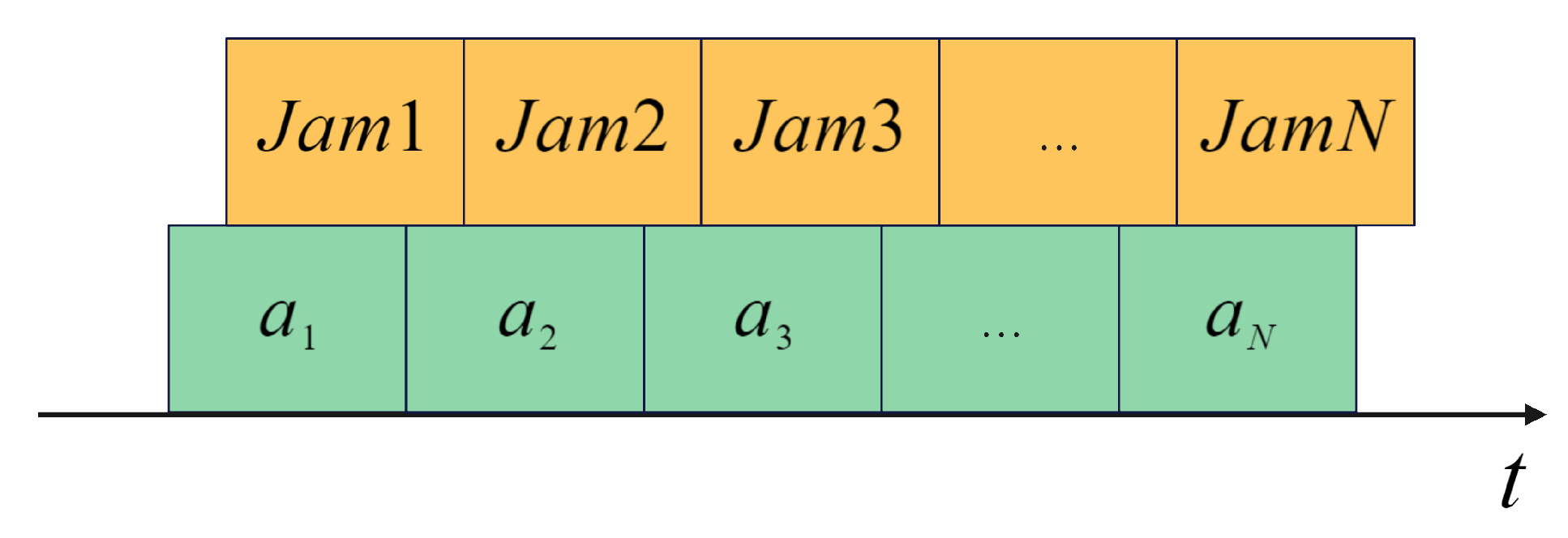
As shown in
Figure 5, this study selects ten game iterations as a complete game process. During the game between the phased-array radar and the jammer, the radar first transmits a detection signal into the environment. After receiving the radar signal, the jammer transmits a jamming signal back toward the radar. The radar then senses the received signal to obtain the state
and subsequently adopts an anti-jamming action,
, based on the current policy,
. This forces the jammer to change its jamming type, resulting in a transition to the next state
.
4.5. Action Space
In this paper, the action space is defined as a discrete set. Since we focus on optimizing anti-jamming strategies over a fixed time interval, the anti-jamming actions must be structured in a “packaged” form. Considering diverse jamming types, this study incorporates frequency agility and cover pulses as active anti-jamming methods, along with the SLC and SLB as passive anti-jamming methods. Accordingly, the action space is formulated as follows:
where
represents either the number of frequency points used in cover pulses or the number of frequency-agility points within one CPI, and when
equals 1, it represents conventional LFM signals. The parameters
and
indicate the activation status of SLC and SLB, respectively.
Specifically, SLB exhibits superior target recovery performance against sidelobe spot jamming, whereas SLC is more effective against coherent slice forwarding jamming. Regarding mainlobe deceptive jamming, only active anti-jamming methods can partially mitigate interference effectively. Additionally, pulse compression is utilized as a fixed action for target detection throughout the anti-jamming decision-making optimization process.
4.6. Reward Function
In RL, the reward function guides the agent in learning the values of different actions when given specific states [
37]. In radar anti-jamming strategy optimization, a suitably designed reward function directly influences training efficiency and the effectiveness of the final policy. An optimal reward function should incentivize the radar system to learn the best anti-jamming strategies, ensuring effective target detection even in complex jamming environments, without misleading the learning process. After reviewing reward function designs in relevant papers [
38,
39,
40], a reward function at both the signal level and data level is designed in this paper. At the signal level, the reward is based on target detection results within a CPI, defined as follows:
where
I denotes the number of pulses within one CPI, and
is calculated as follows:
which indicates that within a CPI, the radar receives a reward of +1 when the
n-th pulse successfully detects the target via CA-CFAR processing, and
otherwise. Target detection is determined by the radar’s estimation of the current environmental situation.
At the data level, the reward function is designed based on
,
,
, and the number of jammed frequency points:
where the gain
quantifies the effectiveness of active anti-jamming measures. The probability of frequency-domain jamming is
. The probability of space-domain jamming is defined as
, with
representing the radar’s maximum detection range and
denoting the estimated distance to the jammer. The passive anti-jamming measure gain is defined as
, where
denotes the
loss resulting from anti-jamming measures.
Considering these signal-level and data-level rewards, the final reward function can be expressed as follows:
In the above equations,
,
,
,
,
, and
represent the weighting factors used to constrain rewards to similar scales. Through RL, the agent progressively discovers the optimal anti-jamming strategy that maximizes the average reward. For comparative purposes, the same reward function is applied to different RL algorithms in simulation experiments. In summary, the pseudocode for the phased-array radar anti-jamming decision-making algorithm based on MAI-DQN is outlined in Algorithm 1.
| Algorithm 1 Training procedure of phased-array radar anti-jamming decision-making |
| Initialize: the state dimension, the size of the action space, hyperparameters for the MAI-DQN, a dueling noisy double evaluation network, the target network with parameters and , priority in the experience pool, the sizes of , , , other parameters for VDDPER, , and , the settings for the phased-array radar and the jammer, and . |
| 1: | for episode = 1 → M do |
| 2: | | if then |
| 3: | | | Generate target echo, random jamming, and noise in the environment, and initialize them as state . |
| 4: | | end if |
| 5: | | Sample a noisy network . |
| 6: | | Choose action . |
| 7: | | Observe the environment again and get as well as . |
| 8: | | Store experience in the shallow experience pool. |
| 9: | | Store experience in the positive deep experience pool or negative experience pool, depending on reward threshold and update if . |
| 10: | | if episode then |
| 11: | | | Sample experience as in the shallow experience pool by probability matrix . |
| 12: | | | Sample the experience as in the positive deep experience pool uniformly. |
| 13: | | | Sample the experience as in the negative deep experience pool uniformly. |
| 14: | | | Integrate the experience in , , into a mini-batch . |
| 15: | | | Update , and . |
| 16: | | | Update through the n-step TD method. |
| 17: | | | Train the evaluation network through backpropagation. |
| 18: | | | Update the priority of the sampling experience by the TD error. |
| 19: | | | Update the sizes of , , and by , as well as . |
| 20: | | | Train the evaluation network using . |
| 21: | | | Update the target network using the soft update method. |
| 22: | | end if |
| 23: | | if then |
| 24: | | | . |
| 25: | | else |
| 26: | | | . |
| 27: | | | Update the type of jamming. |
| 28: | | end if |
| 29: | end for |
5. Experiments
This section presents the simulation results of the phased-array radar anti-jamming decision-making model based on the MAI-DQN. The simulation outcomes are analyzed and discussed to illustrate and validate the effectiveness and performance improvements achieved by the proposed algorithm in the decision-making process. Firstly, the comparison result of the loss function verifies the improvement of the variable learning rate on model training. Secondly, the impact of varying the values of the n-step learning parameter, soft update percentage, discount factor, and noisy network parameter on the average reward is analyzed to validate the chosen hyperparameters. Thirdly, compared with the other algorithms, the performance of MAI-DQN is analyzed from three aspects, that is, reward mean, standard deviation, and average decision accuracy. Fourthly, the pulse compression results using MAI-DQN and DDQN are compared. Lastly, an ablation analysis is conducted to compare the complete MAI-DQN with its variants that exclude improvements. The results demonstrate the effectiveness of the proposed MAI-DQN in phased-array radar anti-jamming decision-making.
5.1. Experimental Settings
In the simulation, the radar is capable of employing the following signal transmission modes: conventional LFM signals, frequency agile signals, and cover pulse signals. The jammer can select from a total of nine jamming types, including mainlobe jamming, sidelobe jamming, and combined mainlobe–sidelobe jamming, such as dense false target jamming, sweep jamming, coherent slice forwarding jamming, and spot jamming. Simulation parameters for radar and jammer settings are presented in
Table 1.
Regarding the RL network structure, this paper adopts two linear network layers as hidden layers, containing 64 units each. The activation function employed in the output layer is the rectified linear unit (ReLU) function [
41], defined as follows:
As one of the classical neural network activation functions, ReLU introduces nonlinearity into the network, enabling neural networks to effectively learn and approximate complex nonlinear relationships. Compared with Sigmoid and Tanh functions, ReLU maintains a constant gradient of 1 within the positive range, providing better gradient propagation and effectively mitigating the vanishing gradient problem. Moreover, ReLU induces sparsity through neuron deactivation, enhancing the model’s generalization capability and reducing overfitting.
Regarding network training, as previously mentioned, this study utilizes VDDPER, an adaptive learning rate, and soft updating of the target network. The detailed parameter settings for the model are presented in
Table 2.
5.2. Experimental Results and Discussion
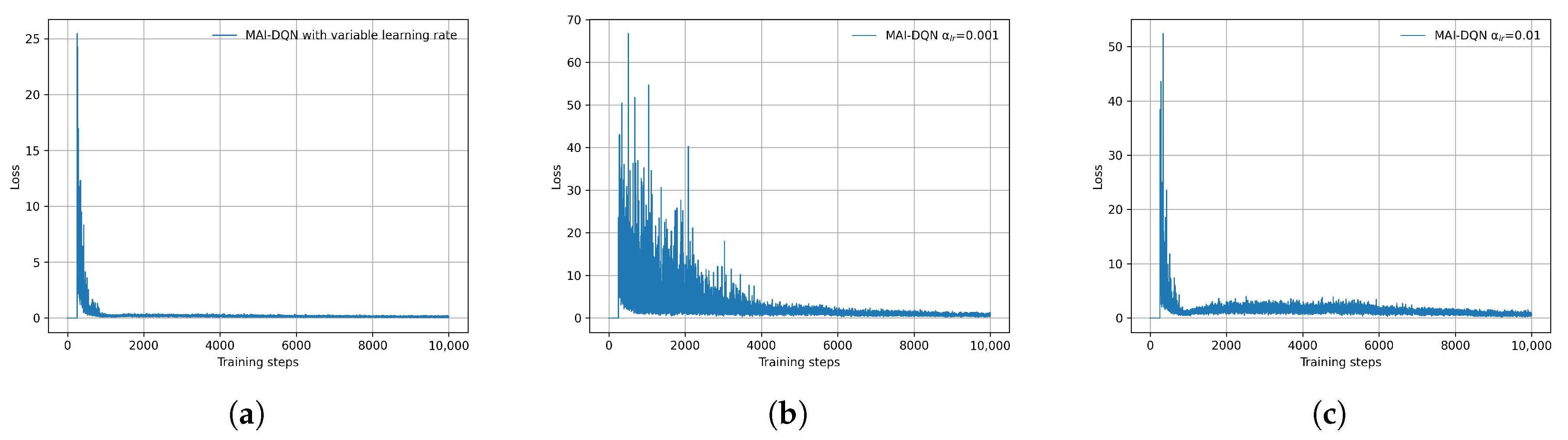
To verify the advantages of using an adaptive learning rate compared to a fixed learning rate, this paper compares their respective loss functions while keeping other parameters of the MAI-DQN model unchanged. As illustrated in
Figure 6, the training convergence achieved by gradually decaying the learning rate
from 0.01 to 0.001 shows significant improvements over fixed learning rates of
= 0.01 and
= 0.001. Specifically, when a fixed learning rate of
= 0.001 is employed, the model’s convergence speed noticeably slows down, requiring approximately 6000 steps to achieve convergence. Conversely, with a fixed learning rate of
= 0.01, although the model initially converges more rapidly, it experiences noticeable oscillations starting at around 1000 training steps.
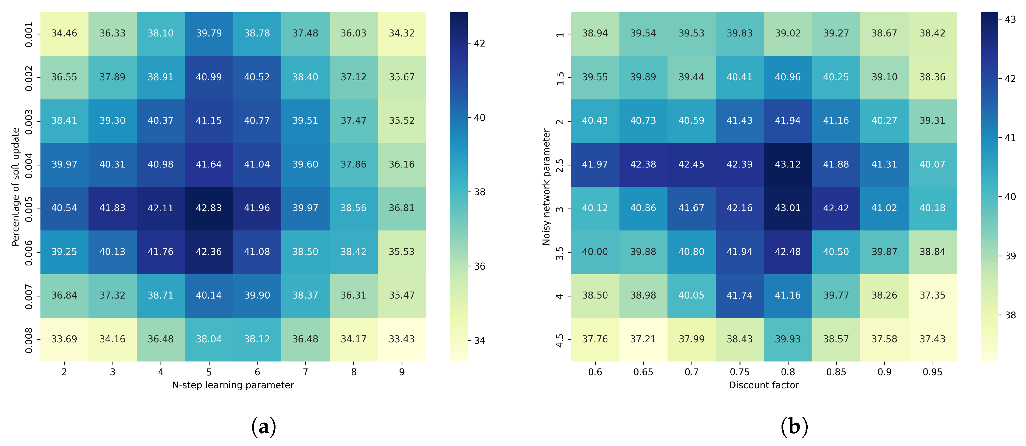
To verify the appropriateness of the hyperparameter settings in this paper, as shown in
Figure 7, we compare the impact of varying the values of the n-step learning parameter, the soft update percentage, the discount factor, and the noisy network parameter on the average reward. The results indicate that when the values listed in
Table 2 are used, the model achieves an optimal average reward.
In terms of the algorithm comparison, the proposed MAI-DQN is compared with four other algorithms, which are Nature DQN, DDQN, the DDPER-VGA-DDQN algorithm proposed by Professor Xiao in [
31], and MAI-DQN using the DDPER instead of VDDPER(MAI-DQN-DDPER). To ensure a fair comparison, all five algorithms share the same neural network parameters, except for the improvements introduced in this paper.
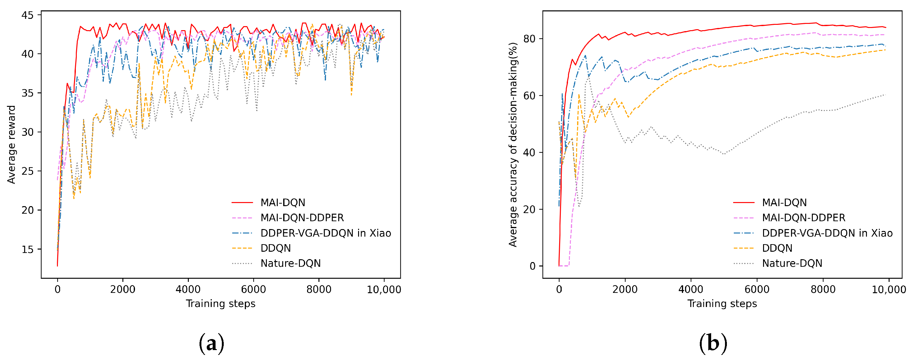
Figure 8a shows the comparison of average rewards during the training process for Nature DQN, DDQN, DDPER-VGA-DDQN, MAI-DQN-DDPER, and the proposed MAI-DQN algorithm.
Firstly, regarding convergence speed, MAI-DQN achieves substantial improvements, reaching convergence at around step 600. In contrast, DDQN and Nature DQN exhibit significantly slower convergence. Meanwhile, MAI-DQN-DDPER and DDPER-VGA-DDQN both converge around step 2200, this notable difference arises because the VDDPER method dynamically adjusts the sampling ratio of experiences with different values during training, thereby enhancing exploratory depth at the initial training stage and significantly accelerating the learning speed.
Secondly, in terms of reward quality and stability, this paper utilizes the mean and standard deviation of rewards to quantify performance, as summarized in
Table 3. Compared with the other four algorithms, MAI-DQN achieves not only rapid convergence but also a higher average reward due to its increased focus on high-value experience in later training stages. Additionally, the multifaceted improvements to the network architecture, particularly the integration of the noisy network structure, result in significantly higher reward stability for MAI-DQN compared to DDQN and DQN.
As shown in
Figure 8b, this paper computes the average decision-making accuracy from the beginning to the end of training to evaluate the decision accuracy of the five algorithms. The results indicate that the MAI-DQN algorithm significantly outperforms MAI-DQN-DDPER, DDPER-VGA-DDQN, DDQN, and Nature DQN in terms of average decision accuracy. Furthermore, a notable performance gap appears between Nature DQN and the other four algorithms, attributable to Nature DQN’s tendency to overestimate
Q-values in complex jamming environments, causing the model to converge to local optima. It should be noted that none of the algorithms reach 100% accuracy post-convergence, as the results include data collected during the initial exploration stage.
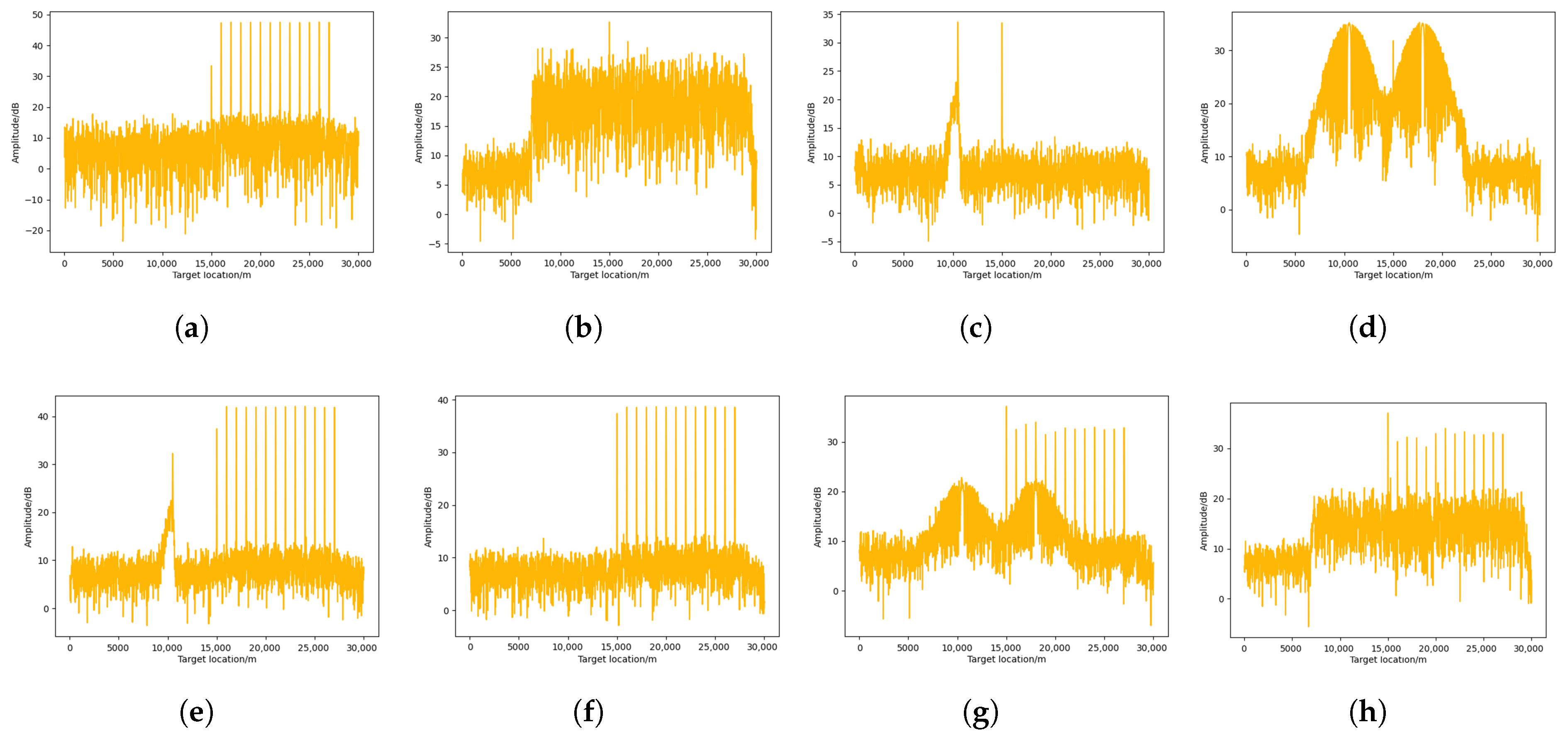
After completing anti-jamming decision-making optimization, this paper compares the pulse compression results using the anti-jamming strategy generated by MAI-DQN with the pulse compression results using the anti-jamming strategy generated by DDQN, thereby validating the effectiveness of the proposed algorithm. To enhance the , the following results are obtained by performing incoherent accumulation of pulse compression within one CPI.
As shown in
Figure 9, the target signal is masked by the jamming signal in the pulse compression output of the jammed phased-array radar system, resulting in a failure to detect the target.
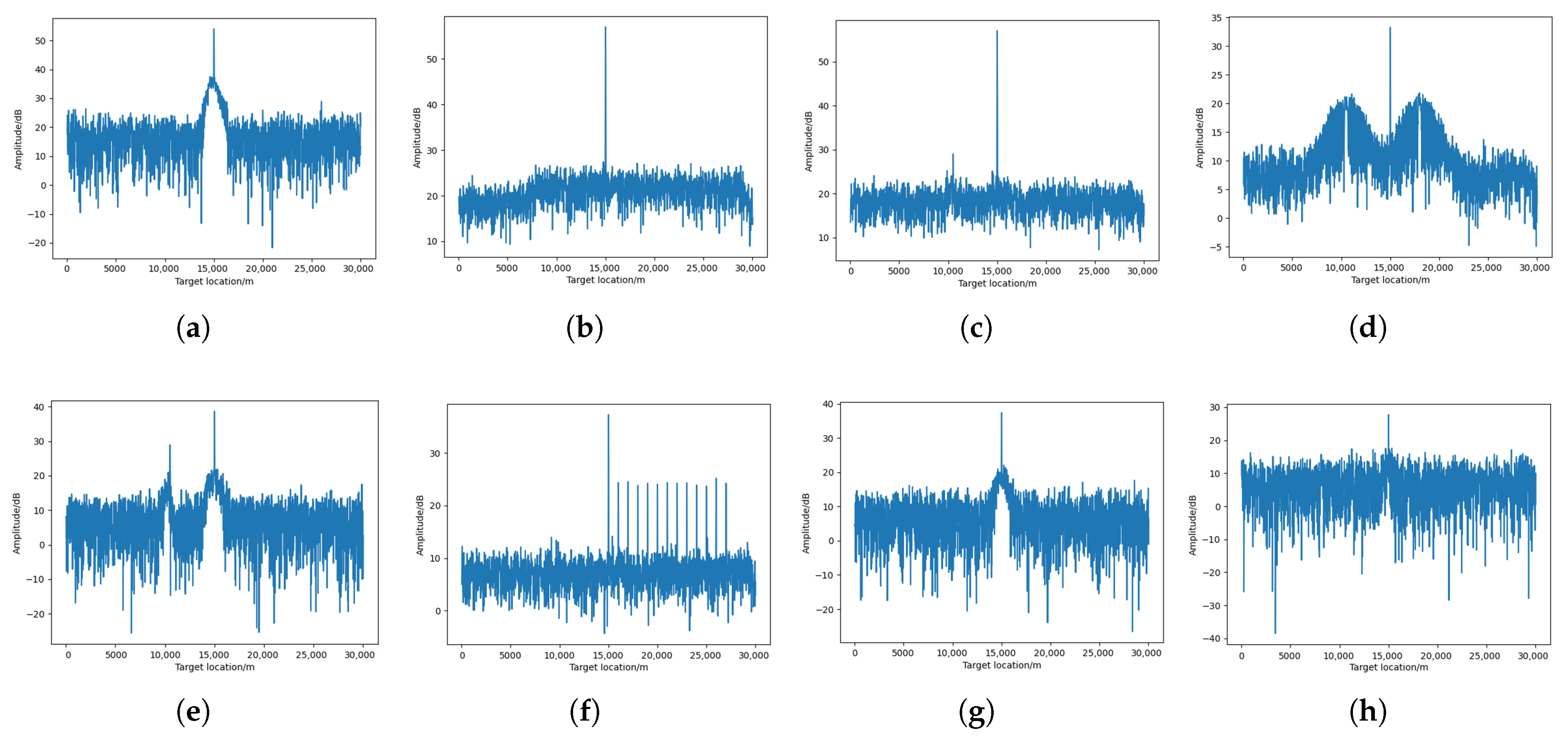
As shown in
Figure 10, in the pulse compression result processed using the anti-jamming strategy generated by MAI-DQN, the target signal is successfully recovered. It is worth noting that although some jamming residue remains in the result, the target can still be detected by CFAR in most cases. However, as shown in
Figure 11, in the pulse compression results processed by the anti-jamming strategy generated by DDQN, the results are affected to varying degrees. Specifically, in
Figure 11a,c–f, the target signals fail to be recovered to a level detectable by CFAR.
As shown in
Figure 12, under 100 Monte Carlo simulations, this paper compares the performance differences among various jamming countermeasures. In the presence of sidelobe jamming or when sidelobe suppression jamming coexists with mainlobe dense false target jamming, the target detection rate achieved after applying the anti-jamming strategies generated by MAI-DQN shows good performance at
levels of 30 dB and below. However, when the
exceeds 30 dB, the detection rates experience a significant decline under all countermeasure settings.
Lastly, as shown in
Table 4, an ablation study was conducted to compare the complete MAI-DQN with its variants that exclude improvements in network architecture, exploration strategy, and training methods, respectively. The comparison focuses on the mean value, standard deviation of the reward, and the average target detection rate after convergence, in order to validate the contribution of each component to the overall model performance. The average target detection rate is obtained from the results of 100 Monte Carlo simulations under all jamming scenarios.
In this paper, the computational hardware includes an Intel(R) Core(TM) i9-12900H CPU @ 2.50 GHz, 32 GB of RAM (Intel, Santa Clara, CA, USA), and an NVIDIA GeForce RTX 3070 Ti Laptop GPU (Nvidia, Santa Clara, CA, USA). The programming environment is Python 3.7, and the framework used is Torch 1.13.1.
Table 5 summarizes the average computational time per decision for the MAI-DQN, DDPER-VGA-DDQN, DDQN, and Nature DQN algorithms during the decision-making process.
Compared to the DDPER-VGA-DDQN algorithm, the MAI-DQN employs a more sophisticated network architecture, resulting in a slightly longer average decision-making time. In contrast, Nature DQN, due to its simpler network structure, achieves the shortest decision-making time among the algorithms. Additionally, because phased-array radar systems typically process larger datasets compared to traditional radars, and given that each decision-making instance in this paper spans one CPI, the single decision time observed here is relatively longer. However, in realistic combat scenarios, anti-jamming strategies are usually generated in advance, thus, the increased decision-making time resulting from the adoption of MAI-DQN is generally acceptable.


