Article

A Node-Degree Power-Law Distribution-Based Honey Badger Algorithm for Global and Engineering Optimization

1
School of Computer Engineering, Jiangsu University of Technology, Changzhou 213001, China
2
College of Information Engineering, Taizhou University, Taizhou 225300, China
3
National Engineering Laboratory for Big Data System Computing Technology, Shenzhen University, Shenzhen 518060, China
*
Author to whom correspondence should be addressed.
Electronics 2025, 14(11), 2302; https://doi.org/10.3390/electronics14112302
Submission received: 31 March 2025 / Revised: 27 May 2025 / Accepted: 3 June 2025 / Published: 5 June 2025
(This article belongs to the Special Issue Applications of Edge Computing in Mobile Systems)

Abstract

The honey badger algorithm (HBA) has gained significant attention as a metaheuristic optimization method; however, despite these design strengths, it still faces challenges such as premature convergence, suboptimal exploration–exploitation balance, and low population diversity. To address these limitations, we integrate a power-law degree distribution (PDD) topology into the HBA population structure. Three improved versions of the HBA are proposed, with each employing different population update strategies: PDDHBA-R, PDDHBA-B, and PDDHBA-H. In the PDDHBA-R strategy, individuals randomly select neighbours as references, promoting diversity and randomness. The PDDHBA-B strategy allows individuals to select the best neighbouring individual, speeding up convergence. The PDDHBA-H strategy combines both approaches, using random selection for elite individuals and best selection for non-elite individuals. These algorithms were tested on 30 benchmark functions from CEC2017, 21 real-world problems from CEC2011, and four constrained engineering problems. The experimental results show that all three improvements significantly improve the performance of the HBA, with PDDHBA-H delivering the best results across various tests. Further analysis of the parameter sensitivity, computational complexity, population diversity, and exploration–exploitation balance confirms the superiority of PDDHBA-H, highlighting its potential for use in complex optimization problems.

1. Introduction

Optimization problems require identification of the optimal solution among a set of feasible alternatives, a type of challenge that is prevalent across various disciplines, including mathematics, computer science, and engineering [1,2]. These tasks often involve maximizing or minimizing a well-defined objective function under specific constraints. Historically, optimization challenges with smooth and continuous characteristics have been addressed via mathematical or gradient-based approaches [3], such as linear programming, quadratic programming, and gradient descent. While effective for simple, differentiable problems, these traditional methods struggle with the complexities of real-world problems, particularly in avoiding local optima and addressing high computational demands [4].
In response to these challenges, metaheuristic algorithms designed to effectively solve complex optimization problems have proliferated over the past few decades [5,6]. These algorithms, which are higher-level procedures inspired by natural phenomena and human cognitive processes, offer significant improvements over traditional methods by guiding the search process towards optimal or near-optimal solutions [7]. They are broadly classified as evolutionary, swarm intelligence, physics-based, or human-inspired algorithms. For example, evolutionary algorithms incorporate natural selection and genetic variation processes, illustrated by strategies such as evolutionary strategies [8], genetic algorithms [9], and differential evolution (DE) [10]. Similarly, swarm intelligence algorithms, such as particle swarm optimization (PSO) [11], the artificial bee colony (ABC) algorithm [12], and the cuckoo search algorithm (CSA) [13], replicate the collective behaviour of organisms. Physics-based methods such as simulated annealing [14], gravitational search [15], and multiverse optimization [16] simulate natural physical phenomena, whereas human-inspired algorithms, including the hiking optimization algorithm [17] and fan optimizer [18], model human cognitive processes.
Swarm intelligence algorithms, a subgroup of metaheuristics, have attracted considerable attention because of their efficacy in addressing complex challenges [19,20]. Introduced in 2022 by Hashim et al., the honey badger algorithm (HBA) exemplifies this phenomenon because of its robust ability to conduct balanced exploration and exploitation, as well as its rapid convergence [21]. This algorithm, inspired by the foraging behaviour of honey badgers, incorporates mechanisms for both intensive local and extensive global searches, aiming to explore the search space effectively and identify optimal solutions. Despite these design strengths, practical applications have shown that HBA can still face challenges such as premature convergence, suboptimal exploration–exploitation balance, and limited population diversity. This motivates further research to enhance its search accuracy, convergence precision, and robustness against local optima. Recent advancements have further refined the capabilities of the HBA. For example, Düzenli et al. incorporated Gaussian mapping and independent learning into the HBA to optimize parameters in photovoltaic models, significantly increasing the precision and robustness of algorithms [22]. Adegboye et al. developed the GST-HBA, which employs tent chaos during the initialization phase and integrates the golden sine mechanism for antenna S-parameter optimization, thereby enriching the diversity of the initial population and improving the global search efficacy [23]. Similarly, Hu et al. augmented the HBA with Bernoulli shift maps, piecewise optimal decreasing neighbourhood strategies, and adaptive level crossing for unmanned aerial vehicle path planning, increasing the pathfinding efficiency and reliability [24]. Additionally, Asha et al. adapted the HBA to train IoT performance prediction models using recurrent neural networks, improving the training efficiency and predictive accuracy [25]. Nassef et al. enhanced the HBA via dimension learning-based hunting for maximum power point tracking in global optimization, which resulted in superior identification of global optima [26]. Moreover, Abasi et al. employed quasi-oppositional learning, arbitrarily weighted proxies, and adaptive mutation strategies in the HBA to optimize the hyperparameters of convolutional neural networks, markedly accelerating convergence and increasing accuracy [27].
The integration of complex network topologies has also been recognized as a method for enhancing the performance of optimization algorithms by improving information exchange and collaboration within populations [28,29]. For example, Gong and Zhang enhanced PSO by integrating small-world networks, which improved particle information exchange, convergence rates, and solution quality [30]. Ni et al. introduced a dynamic stochastic population topology in PSO for generalized portfolio selection, increasing the algorithm’s adaptability and flexibility in response to market changes [31]. Additionally, Huang et al. utilized small-world networks in DE to create dynamic neighbourhoods, enhancing the ability of the algorithm to escape local optima by altering intrapopulation dynamics [32]. Wang et al. applied a scale-free topology in the salp swarm algorithm to map follower relationships, which boosted performance by enabling more effective information sharing [33]. Similarly, Ji et al. enhanced the ABC by restricting bee neighbour interactions within a scale-free network, thereby increasing the search capabilities [34]. Furthermore, Yu et al. incorporated a complex network topology in the mutation operator of DE to effectively avoid local optima, thereby increasing the algorithm’s robustness and reliability [35].
The above studies have shown the integration of complex networks into optimization algorithms to be a promising direction. Among them, the power-law degree distribution (PDD) topology, which is characterized by many low-degree nodes and a small number of high-degree hubs, is particularly suitable for modelling networks that rely on hub-based communication and efficient information propagation. Moreover, the superiority of PDD over other complex network structures when applied to optimization algorithms has been demonstrated in [34,35]. Building upon these insights, this paper introduces three innovative strategies to refine the HBA by employing a PDD structure for the HBA population. With the PDD topology, individuals engage in information exchange exclusively with their connected neighbours. The main contributions of this study are as follows:
  • This study innovatively incorporates a PDD structure to model the interaction topology of the HBA population, where individuals exchange information exclusively with their connected neighbours. This design better simulates complex real-world network interactions, enhancing algorithm adaptability.
  • Three interaction strategies are proposed: (i) PDDHBA-R, which employs roulette selection to randomly choose neighbours for information exchange, increasing the population diversity and exploration capability; (ii) PDDHBA-B, which strategically selects the most promising neighbour to accelerate convergence; and (iii) PDDHBA-H, a hybrid approach that divides the population into elite and non-elite groups and applies different interaction mechanisms to effectively balance exploration and exploitation.
  • The comparative experiments demonstrate that PDDHBA-H significantly outperforms other HBA variants and mainstream metaheuristic algorithms in terms of optimization performance, population diversity, and convergence efficiency, highlighting its effectiveness in balancing exploration and exploitation.
The remainder of this paper is organized as follows: Section 2 describes the foundational principles of the HBA. Section 3 explores the Barabási–Albert (BA) model used to generate power-law distribution networks. Section 4 outlines the motivation for the proposed improvements and presents the three strategies in detail. Section 5 provides a comprehensive review of the experimental results. Section 6 offers an in-depth analysis of the PDDHBA-H approach. Finally, Section 7 concludes the research and discusses future research directions.

2. Honey Badger Algorithm

The HBA is an optimization algorithm inspired by the foraging behaviour of honey badgers. The researchers who developed this algorithm identified two distinct behavioural phases in the foraging process of honey badgers: the digging phase and the honey phase. In the digging phase, honey badgers use their keen sense of smell to detect prey. When they are near the prey, they explore the vicinity in a trajectory that resembles a heart shape. During the honey phase, honey badgers collaborate with honey-guide birds, which are responsible for locating beehives. The birds pinpoint the locations, and the badgers subsequently extract the honey.

Numerical Expression of the HBA

Because it involves exploration and exploitation phases, the HBA is classified as a global optimization algorithm. It represents each candidate solution as a one-dimensional vector, similar to other population-based algorithms. Assuming a population size of N P and a problem dimension of D, the HBA population is mathematically expressed as follows:
P O P = x 1 , 1 x 1 , 2 x 1 , D x 2 , 1 x 2 , 2 x 2 , D x N P , 1 x N P , 2 x N P , D
Here, x i = [ x 1 , 1 , x 1 , 2 , . . . , x 1 , D ] represents the position of the ith honey badger. The optimization process comprises four main stages: initialization, population evaluation, specific coefficient calculation, and population updating.
(1) Initialization stage: Initially, the positions of the honey badgers are randomly generated via the following equation:
x i , j = L B j + r 1 × ( U B j L B j ) , j = 1 , 2 , . . . , D ,
where r 1 is a random number between 0 and 1 and where L B j and U B j are the lower and upper bounds of the search space, respectively.
(2) Population evaluation stage: For each honey badger position, its fitness value is computed, and the position with the best fitness, denoted as x b e s t (prey), is identified.
(3) Specific coefficient calculation stage: This stage involves calculating three crucial coefficients: the olfactory strength coefficient (I), density coefficient ( α ), and direction flag coefficient (F). The value of I is determined by the prey concentration and the distance between the ith honey badger and the prey. This value is defined by an inverse square law, as shown in Figure 1, and is computed using the equations below:
I i = r 2 × S 4 π d i 2 ,
where S = ( x i + 1 x i ) 2 and d i = x b e s t x i . Here, r 2 is a random number between 0 and 1, S represents the prey concentration, and d i denotes the distance between the prey and the ith honey badger. The density coefficient α , which is commonly used in optimization algorithms, decreases with increasing iterations. It is calculated as follows:
α = K × e x p ( T T m a x ) ,
where T m a x is the maximum number of iterations and where K is a constant greater than 1, typically set to 2. Given that each iteration involves evaluating a population of size NP, when the termination criterion is defined by the maximum number of function evaluations (maxFEs), the number of iterations can be calculated as T m a x = m a x F E s / N P . The direction flag variable F is used to change the search direction and is calculated as follows:
F = 1 , if r 3 0.5 , 1 , otherwise ,
where the value of F is determined by comparing the random variable r 3 (ranging from 0 to 1) to the threshold 0.5.
(4) Population update stage: The population update stage simulates the two hunting modes of the honey badger. In the digging mode, the movement of a honey badger resembles a cardioid curve (see Figure 2), and the new position of a honey badger can be represented as follows:
x i = x b e s t + F × β × I × x b e s t + F × r 4 × α × d i × | c o s ( 2 π r 5 ) × ( 1 c o s ( 2 π r 6 ) ) | ,
where β is a constant greater than 1, typically set to 6, representing the predation capability of the honey badger. r 4 , r 5 , and r 6 are three distinct random numbers (between 0 and 1). In the honey mode, the new position of the honey badger is calculated as follows:
x i = x b e s t + F × r 7 × α × d i ,
where r 7 is a random number between 0 and 1. In each iteration of the HBA, the digging mode and honey mode are randomly selected with a 50% probability, where the former corresponds to the exploration process and the latter corresponds to the exploitation process of the optimization algorithm. To provide a clear depiction of the HBA optimization process, Algorithm 1 outlines the pseudocode for its implementation.
Algorithm 1: Pseudocode of the HBA
Electronics 14 02302 i001

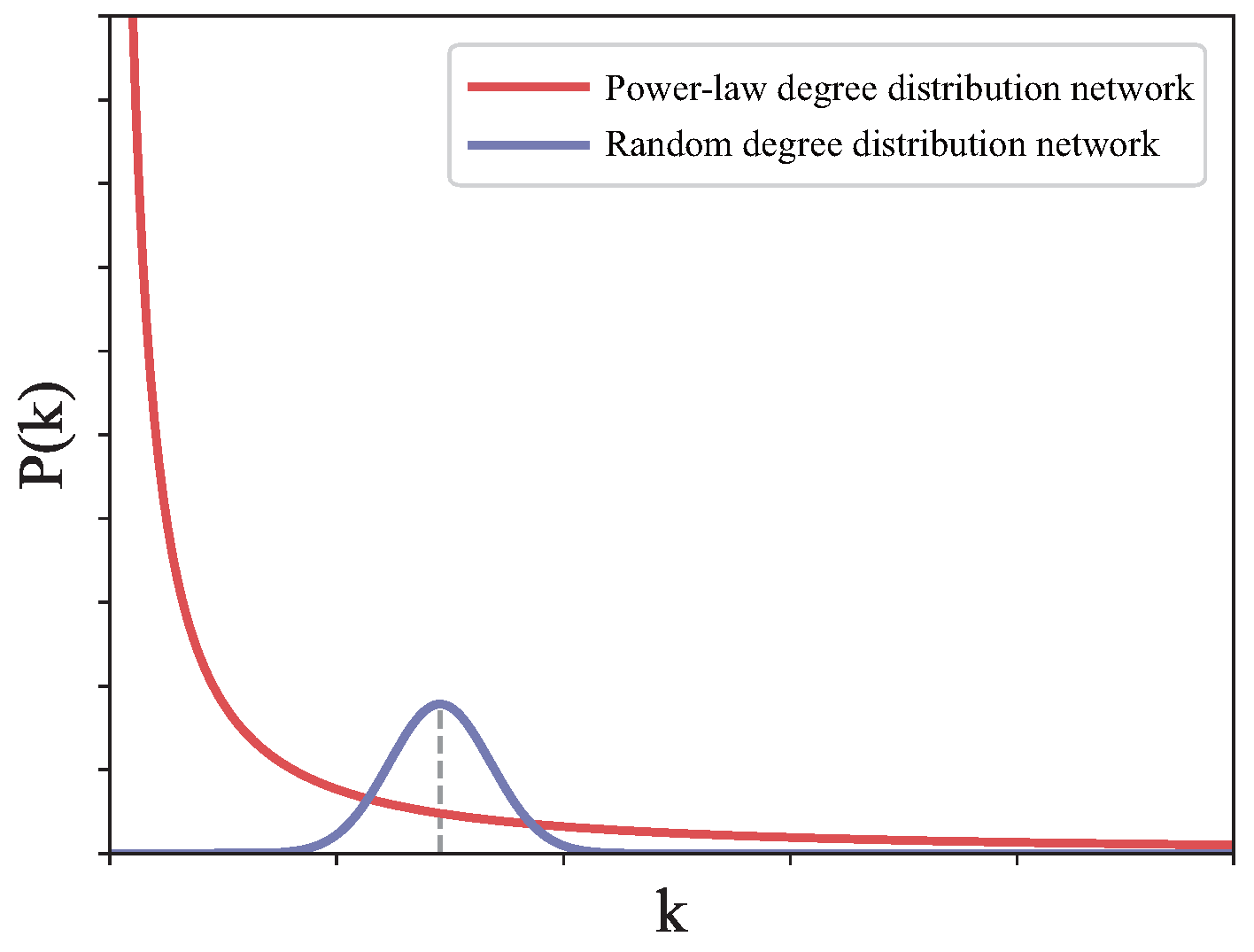
3. Barabási–Albert (BA) Model

The BA model, proposed by Barabási et al. in 1999, characterizes a variety of complex systems, including the Worldwide Web, social networking sites, and financial networks [36]. A defining feature of these networks is their adherence to a power-law distribution of node degrees, in which there are many low-degree nodes along with a small number of high-degree nodes. For any node in the network, the probability P ( k ) of having degree k adheres to the following relation:
P ( k ) k γ ,
where γ denotes the scaling exponent, which is generally between 2 and 3. In contrast, traditional random networks exhibit a degree distribution approximating a Poisson distribution, characterized by node degrees concentrated around a mean value [37,38]. To clearly illustrate these differences, Figure 3 and Figure 4 depict their structural diagrams and degree distribution curves, respectively. It is evident that random networks have relatively uniform degree distribution, whereas in BA model-based networks, only a few nodes have very high degrees. These highly connected nodes, also known as hubs, often play pivotal roles in processes such as information dissemination, influence propagation, and resource allocation. The process of constructing a PDD network via the BA model is governed by two mechanisms: the growth mechanism and the preferential attachment mechanism. The growth mechanism continuously adds new nodes over time, beginning with a small initial set of nodes. The preferential attachment mechanism describes the tendency of new nodes to preferentially attach to nodes with higher degrees in the network, exemplifying the “rich get richer” Matthew effect. The process of generating a PDD network with NP nodes via the BA model is outlined as follows:
Step 1: Construct a fully connected network comprising M nodes.
Step 2: Calculate the probability values for all nodes in the current network; the probability P i for node i is computed as P i = d ( i ) / j d ( j ) , where d ( i ) denotes the degree of node i.
Step 3: Add a new node to the network and select its attachment point on the basis of the probability P i .
Step 4: Iteratively repeat steps 2 and 3 until the N P th node is added to the network.

4. Power-Law Degree Distribution Topology-Based HBAs

4.1. Motivation

The original HBA enhances the optimization process by incorporating distinct phases for exploration and exploitation. However, as shown by Equations (6) and (7), the individual update mechanisms in the HBA depend on the best individual, x b e s t . When x b e s t represents the global optimum, there is rapid convergence towards the optimal solution. Conversely, if x b e s t is trapped in a local optimum, this leader biases the entire population towards a suboptimal solution. Additionally, this update strategy, which focuses on the leading individual, decreases population diversity and overlooks the potential for information exchange among population members. Therefore, refining the individual update strategies within the HBA is imperative. In our research, we use nodes in a PDD network to mirror individuals in the HBA population, thereby creating a network topology. In this topology, a small number of individuals have numerous connections, whereas the majority have few connections. Considering that the optimal individual in the population is more likely to discover the best solution, we arrange the population in ascending order of fitness, assuming that this is a minimization problem. Each individual is subsequently mapped to a node in the network, and these nodes are sequentially numbered according to their integration into the network. The updating of an individual’s position no longer depends on x b e s t but rather on the individual’s topological neighbours. We propose three individual learning strategies to improve the performance of the HBA.

4.2. Random-Neighbour-Based Strategy: PDDHBA-R

This strategy enables each individual to randomly select a topological neighbour as the reference target for its update process. Accordingly, Equations (6) and (7) in the original HBA are modified as follows:
x i = x r n + F × β × I × x r n + F × r 4 × α × d i × | c o s ( 2 π r 5 ) × ( 1 c o s ( 2 π r 6 ) ) | ,
x i = x r n + F × r 7 × α × d i ,
where x r n denotes an adjacent individual who is randomly selected for individual x i . This approach, akin to the improvement Ji et al. made to the ABC algorithm [34], randomly provides different references for each individual, thus reducing the risk of rapid convergence to local optima and slowing the reduction in population diversity. In the PDD topology, node connections can be classified into two cases, as illustrated in Figure 5. In the first case, x i has multiple neighbours, but only one of them is superior. As a result, x i is more likely to select an inferior neighbour. The second case is a more common situation, where x i has only one better neighbour. Whereas case 2 can improve the performance of the HBA, case 1, as shown in Figure 5a, is theoretically expected to degrade its performance.

4.3. Best-Neighbour-Based Strategy: PDDHBA-B

To address the problem of frequently selecting inferior individuals in PDDHBA-R, we introduce the PDDHBA-B algorithm. This approach ensures that each individual selects the optimal neighbouring individual, denoted as x b n , as the reference individual. Consequently, in Equations (9) and (10) of PDDHBA-R, x b n replaces x r n to represent the best adjacent individual. PDDHBA-B prevents reliance on x b e s t as a universal reference and eliminates the high likelihood of individuals choosing worse references in PDDHBA-R.

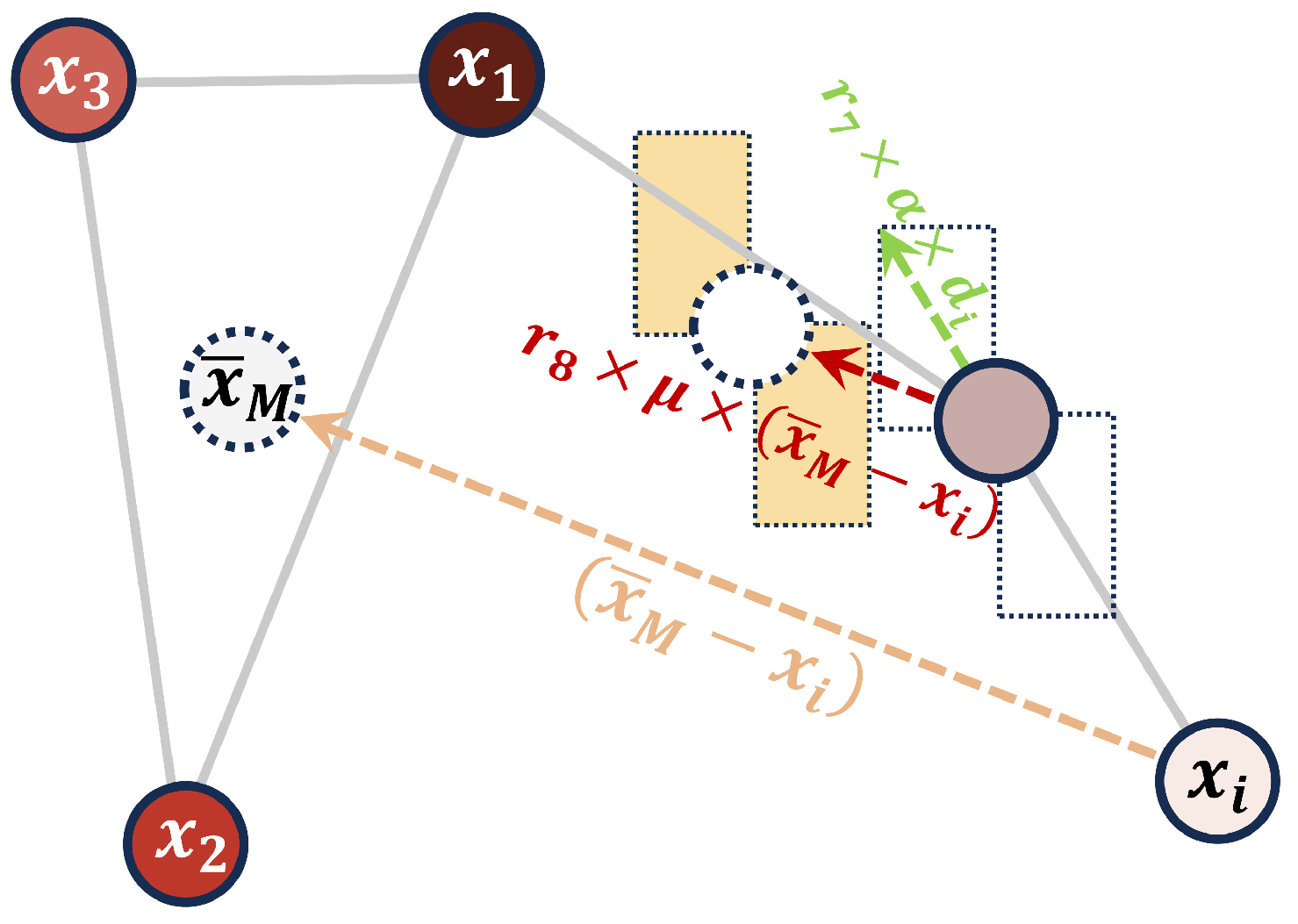
4.4. Hybrid Strategy: PDDHBA-H

The third strategy, PDDHBA-H, combines the first two strategies by dividing the population into two distinct groups: an elite group, comprising the first M individuals, and a non-elite group, consisting of individuals numbered M + 1 to N P . Within the elite group, each individual is fully interconnected and randomly selects another member from this group as a reference. Conversely, individuals in the non-elite group select their best adjacent individual as a reference. Consequently, the mining mode in PDDHBA-H is defined as follows:
A = F × β × I , B = F × r 4 × α × d i × cos ( 2 π r 5 ) × ( 1 cos ( 2 π r 6 ) ) , x i = x r n + A × x r n + B , if i M , x b n + A × x b n + B , otherwise ,
where x r n and x b n represent the randomly selected and best adjacent individuals of x i , respectively. Inspired by the grey wolf optimizer (GWO) [39], an offset term is incorporated into the update formula for all individuals, shifting the search area towards the centre of the elite group. Equation (7) of the original HBA is improved as follows:
x i = x r n + F × r 7 × α × d i + r 8 × μ × ( x ¯ M x i ) , if i M , x b n + F × r 7 × α × d i + r 8 × μ × ( x ¯ M x i ) , o t h e r w i s e ,
where r 8 is a random number between 0 and 1. μ is a constant less than 1, and setting it to 0.2 aims to induce a slight shift of the search area towards the centroid of the elite population. This choice means that the algorithm will focus slightly more on the region around the elite individuals while still maintaining a certain level of search diversity. A schematic diagram of this offset is shown in Figure 6. For a clearer illustration of the proposed algorithms’ processes, Figure 7 presents a flowchart of the HBA incorporating three different strategy improvements based on a PDD network. Algorithm 2 gives the pseudocode of the PDDHBA-H.
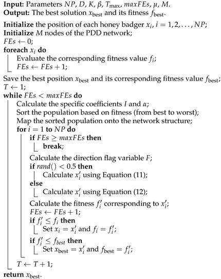
Algorithm 2: Pseudocode of PDDHBA-H
Electronics 14 02302 i002

5. Experimental Study

To assess the efficacy of the proposed algorithms, we utilized the well-known and challenging CEC2017 benchmark functions [40]. We conducted comprehensive comparative experiments, including an analysis of PDDHBA-H against the original HBA, six HBA variants from the literature, and seven other metaheuristic algorithms.

5.1. Benchmark Functions and Experimental Setup

The CEC2017 benchmark functions are a set of 30 complex optimization problems that include unimodal, simple multimodal, hybrid, and composite functions. These problems are designed to mimic a variety of real-world optimization challenges and are commonly employed to evaluate the effectiveness of optimization algorithms. Functions F1–F3, which are unimodal and primitive, test the local search capabilities of the algorithms. Functions F4–F10, which involve avoiding multiple local optima, assess the global search ability. The ten hybrid functions, F11–F20, are crafted by integrating various simple functions to examine performance in more complex scenarios. Functions F21–F30, as composite functions, are used to evaluate algorithms in diverse and intricate settings. Owing to the instability of the F2 function, we used only the other 29 functions from CEC2017.
To ensure equitable performance comparisons, we standardized the stopping criteria across all algorithms at a maximum of 10 5 function evaluations, with a population size of 50 and a search range of [−100, 100]. We considered dimensions of 30, 50, and 100 to assess algorithm performance thoroughly. To reduce variability and enhance reliability, 30 independent runs of each algorithm were performed. All testing was executed on a personal computer equipped with a 3.7 GHz Intel(R) Core(TM) i9-10900K CPU and 32 GB of RAM using MATLAB R2020a.

5.2. Performance Evaluation Metrics

Mean and standard deviation (Std) of the final fitness values (30 runs): This metric quantifies the average performance level and stability of the algorithms over multiple runs. The mean reflects the typical outcome, and the standard deviation captures variability, providing insight into the reliability of the algorithm.
Two-sided Wilcoxon rank-sum test: This nonparametric test determines whether there are statistically significant differences between the distributions of two independent samples [41]. We set the significance level at α = 0.05 . The outcomes are reported in a “win/tie/lose” (w/t/l) format, where “w” denotes the number of instances in which the control algorithm significantly outperforms the competing algorithm, “l” indicates inferior performance, and “t” indicates that there is no significant difference.
Friedman test: This robust nonparametric statistical method is used to compare the rankings of algorithms across multiple datasets or functions [42]. In this test, a lower ranking indicates better performance. The Friedman test is particularly useful when comparing more than two algorithms or datasets.
Convergence curve: This graphical representation illustrates the progression of fitness values over iterations. By comparing the convergence curves of different algorithms plotted on the same graph, we can visually assess differences in convergence rates, stability, and achievement of optimal fitness levels.
Box plot: This plot is used to illustrate the distribution of fitness values across multiple runs for each algorithm. It depicts the minimum, first quartile (Q1), median, third quartile (Q3), and maximum values, offering a clear visual summary of the central tendency, spread, and presence of outliers in the performance data.
Each of these metrics provides distinct insights into the performance of the algorithms, facilitating a comprehensive assessment of their efficacy and robustness in solving optimization problems.

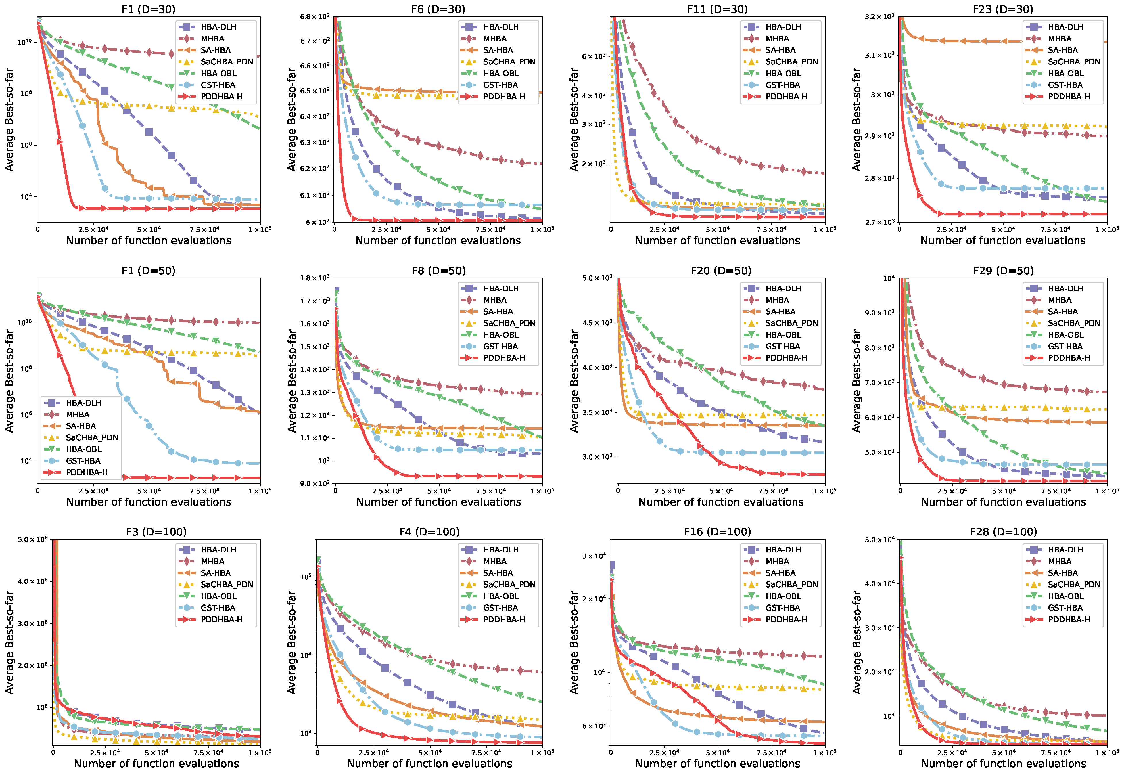
5.3. Comparison of Experimental Results

In this subsection, we compare the three proposed improved HBA variants with the original HBA. The statistical results for the 30-dimensional, 50-dimensional, and 100-dimensional problems are presented in Table 1, Table 2, and Table 3, respectively, where the best results for each algorithm are highlighted in bold. Table 1 shows that PDDHBA-H achieves the best results in 18 cases, whereas the HBA obtains the best results in 2 cases. PDDHBA-B and PDDHBA-R achieve the best results in 3 and 6 cases, respectively. According to the results of the two-sided Wilcoxon rank-sum test in Table 1, PDDHBA-H outperforms the HBA in 19 cases, PDDHBA-B in 12 cases, and PDDHBA-R in 8 cases. In contrast, PDDHBA-H performs worse than the other algorithms in only two cases. In the 50-dimensional setting, PDDHBA-H again achieves the greatest number of top results, 15 in total. PDDHBA-R ranks second with the best results in nine cases. In the two-sided Wilcoxon rank-sum test, PDDHBA-H significantly outperforms the HBA in 20 cases, PDDHBA-B in 15 cases, and PDDHBA-R in 8 cases. Moreover, PDDHBA-H performs significantly worse than the HBA in only two cases; and in two cases, PDDHBA-H is outperformed by PDDHBA-R. PDDHBA-H does not significantly perform worse than PDDHBA-B in any of the cases. According to the results presented in Table 3, PDDHBA-H continues to demonstrate the best performance, achieving the best result in 17 cases. PDDHBA-H significantly outperforms the other algorithms in 22, 12, and 11 cases but has a significant disadvantage in 2, 0, and 1 cases, respectively. The Friedman test ranks the algorithms consistently across all dimensional settings (Table 1, Table 2 and Table 3) in the following order: PDDHBA-H > PDDHBA-R > PDDHBA-B > HBA. To further illustrate these differences, Figure 8 presents convergence graphs for representative functions. These graphs show that PDDHBA-B, PDDHBA-R, and PDDHBA-H generally achieve better convergence than HBA does. Specifically, PDDHBA-H combines rapid convergence with robust outcomes, whereas PDDHBA-B exhibits rapid convergence, although it occasionally experiences premature convergence. On the other hand, PDDHBA-R demonstrates slower but steadier convergence. To summarize, all three improved versions of the HBA outperform the original, with PDDHBA-H, which integrates both best-neighbour and random-neighbour strategies, showing the most significant improvements.
To verify the effectiveness of the proposed best strategy, PDDHBA-H, a comparison was made with six HBA variants: HBA-DLH, MHBA, SA-HBA, SaCHBA_PDN, HBA-OBL, and GST-HBA [22,23,24,25,26,27]. All algorithms used the same common parameters set for the original HBA, and each variant’s specific hyperparameters were adjusted according to their respective foundational papers. The statistical results for 30, 50, and 100 dimensions are displayed in Table 4, Table 5 and Table 6. PDDHBA-H consistently outperformed the other variants, as evidenced by its superior mean and standard deviation scores and its improved performance on 22, 24, and 24 functions for 30, 50, and 100 dimensions, respectively. Notably, PDDHBA-H was superior to the other variants, showing weaker performance on no more than two functions in any dimension. The Friedman test consistently ranked PDDHBA-H as superior across all dimensions, highlighting its robust performance. Figure 9 shows the convergence curves of PDDHBA-H versus other variants on representative functions, demonstrating faster convergence rates. Additionally, Figure 10 presents box plots from 30 experimental runs per algorithm on selected functions; the optimal and robust performance of PDDHBA-H is demonstrated by its achievement of the lowest medians and narrowest interquartile ranges across most functions. Overall, these results confirm that the introduction of strategic novelty markedly improves the HBA performance, leading to significant robustness in its optimization performance.
In addition to evaluating PDDHBA-H against various HBA variants, we compared it with seven metaheuristic algorithms to further validate its performance. These algorithms include three classic algorithms, namely, particle swarm optimization (PSO), differential evolution (DE), and the cuckoo search algorithm (CSA), and four recent algorithms, namely, the grey wolf optimizer (GWO), whale optimization algorithm (WOA), sparrow search algorithm (SSA), and dung beetle optimizer (DBO), which have garnered significant attention [10,13,39,43,44,45]. To ensure fair comparisons, all algorithms were configured with identical parameter settings derived from the relevant literature, as detailed in Table 7. The statistical results for 30, 50, and 100 dimensions are presented in Table 8, Table 9 and Table 10, respectively. For the 30-dimensional functions, PDDHBA-H demonstrated superior performance, achieving the best solutions for 16 functions, whereas the next highest, DE, achieved the best results for 7 functions. The Wilcoxon rank-sum test results, which are provided in Table 8, support the superior performance of PDDHBA-H. Specifically, PDDHBA-H significantly outperformed PSO on 23 functions and matched it on 4 functions. Compared with DE, it was superior for 22 functions and inferior for 6. Compared with the GWO, PDDHBA-H had a significant advantage for 22 functions and was outperformed by the GWO on only 1 function. The WOA, SSA, and DBO did not significantly outperform PDDHBA-H on any function, whereas PDDHBA-H outperformed them on 29, 22, and 27 functions, respectively. The CSA was the closest in performance, achieving a Friedman ranking of 2, just behind PDDHBA-H’s ranking of 1. PDDHBA-H significantly outperformed the CSA on 17 functions and was inferior to it on 6 functions. For the 50-dimensional functions, PDDHBA-H again led to the best solutions for 23 functions, whereas the remaining best results were obtained by PSO, DE, and the GWO for 1, 4, and 1 functions, respectively. In the 100-dimensional assessments, PDDHBA-H maintained a robust performance advantage, obtaining the best solutions for 21 functions. It significantly outperformed PSO, DE, the GWO, the WOA, the SSA, the DBO, and the CSA on 26, 29, 25, 29, 22, 27, and 29 functions, respectively, as detailed in Table 10. Figure 11 shows the convergence curves for all the algorithms. PDDHBA-H consistently demonstrated rapid convergence and excelled in achieving superior outcomes for the majority of functions. While some algorithms achieved faster convergence rates on a few functions, they predominantly exhibited premature convergence to local optima. To further assess the solution quality, Figure 12 displays box plots for each algorithm. PDDHBA-H consistently obtained the lowest median values and narrower interquartile ranges across most functions, underscoring its role in improving HBA performance.

6. Discussion

6.1. Parameter Sensitivity

On the basis of prior discussions, the construction of the PDD network begins with a fully connected network of M nodes. The value of M not only determines the topology but also influences adjacency relationships among individuals in the population, which are crucial for the optimization performance of the PDDHBA-H algorithm. Parameter tuning is a critical aspect of optimizing metaheuristic algorithms and can be performed either manually or through automated methods. Manual tuning leverages expert knowledge to iteratively adjust key parameters, typically those with limited value ranges, and generally requires lower computational resources. In contrast, automated tuning techniques—such as CRS-Tuning, F-Race, REVAC, and ParamILS—systematically explore the parameter space to identify near-optimal configurations, particularly effective when multiple parameters are involved; however, these methods often demand substantially higher computational cost and time. Given that the parameter M is an integer constrained within a relatively narrow range, manual tuning was deemed a practical and efficient approach to thoroughly assess its influence on the algorithm’s performance. Figure 13 illustrates the average degree distribution of the PDD network for various values of M. The results indicate that the first M nodes have higher degrees, whereas nodes from M + 1 to the end of the network have significantly lower degrees. These first M nodes correspond to the elite group in the PDDHBA-H population, whereas the remaining nodes correspond to the non-elite group. Thus, changing M effectively adjusts the proportion of elite groups compared to non-elite groups.
To investigate the impact of M on PDDHBA-H’s performance, we varied M from 2 to 25 and conducted 30 rounds of experiments on the CEC2017 test set. Figure 14 presents the Friedman test ranking results for different values of M under 30-dimensional, 50-dimensional, and 100-dimensional conditions. According to Figure 14, the optimal values of M for 30D, 50D, and 100D are 10, 15, and 23, respectively. Furthermore, as M increases, the algorithm’s performance initially improves and then decreases, with the performance peak decreasing as the problem dimension increases.

6.2. Computational Complexity

Determining the computational complexity is essential for gauging the efficacy of an algorithm. Let D be the dimension of the problem to be optimized, N be the population size, and T be the maximum number of iterations. The computational complexity of the original HBA is analysed as follows: the complexities of the population initialization and fitness evaluation are O ( N D ) and O ( N ) , respectively. The complexities of α , I, and F are O ( T ) , O ( T N ) , and O ( T N ) , respectively. In the main loop, the complexities of the population fitness evaluation and update are O ( T N ) and O ( T N D ) , respectively. Hence, the overall complexity of the HBA is O ( N D + N + T ( 1 + 3 N + N D ) ) , which is simplified to O ( T N D ) .
For the PDDHBAs, additional complexity arises from population sorting and the creation of the PDD network. The complexity of constructing the PDD network is O ( N l o g ( N ) ) , and that of population sorting is O ( T N l o g ( N ) ) . Thus, the computational complexity of PDDHBAs is O ( N D + N + N l o g ( N ) + T ( 1 + 3 N + N D + N l o g ( N ) ) ) , which is simplified to O ( T N ( D + l o g ( N ) ) ) . This analysis shows that the PDDHBAs have slightly greater computational complexity than the HBA, but their performance is substantially improved. Therefore, the PDDHBAs are computationally more efficient than the HBA.

6.3. Search History, Diversity, and Exploration–Exploitation Analysis

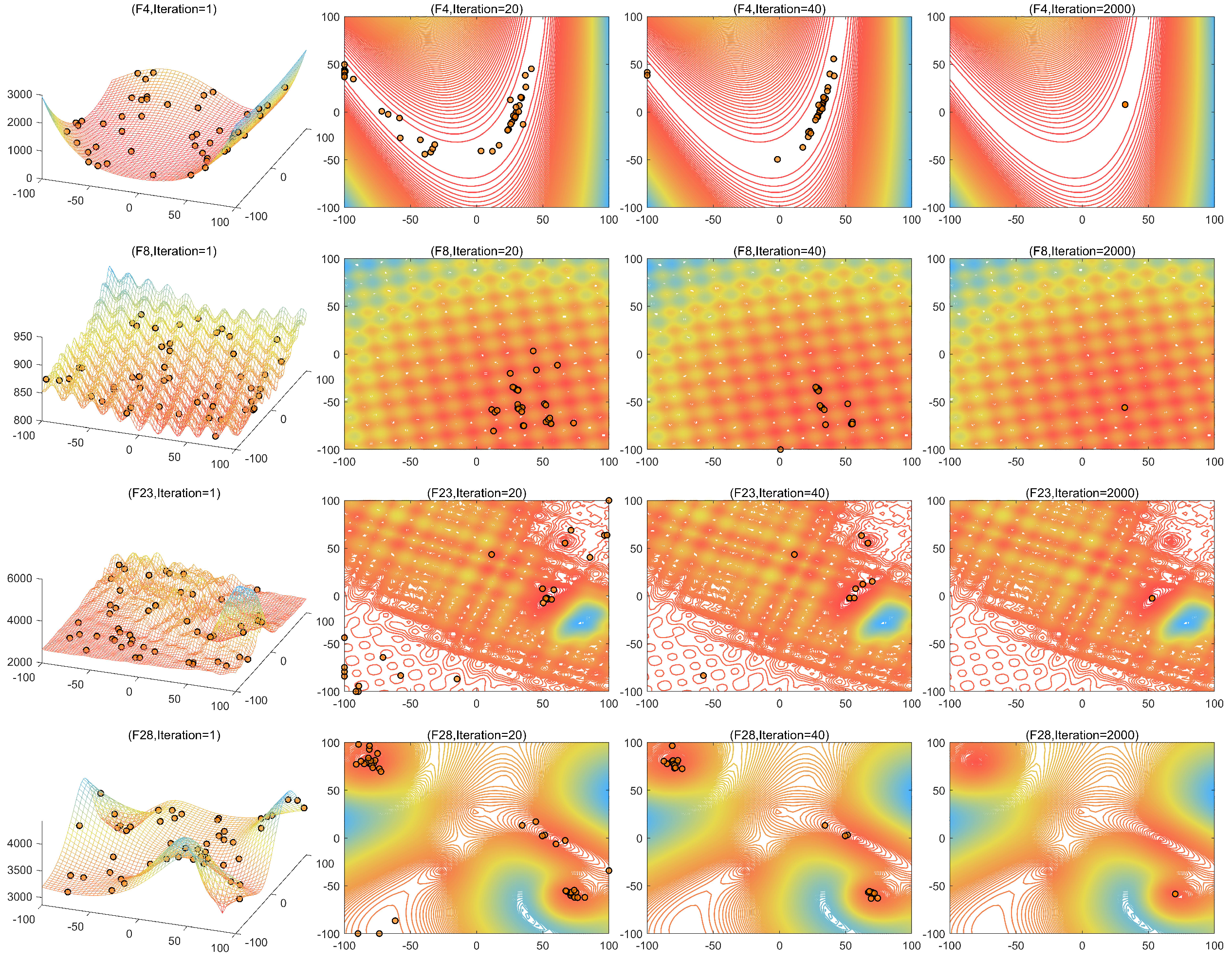
6.3.1. Search History Analysis

The population search history can be utilized to evaluate the robustness and search performance of an algorithm [48]. Here, the CEC2017 test function set was employed, and experiments were conducted with a population size of 50 and a maximum of 2000 iterations. Figure 15 illustrates the population search history for four representative functions (F4, F8, F23, and F28). As depicted in Figure 15, in iteration 1, the population is dispersed across the entire search space. For the unimodal function F4, the population clusters around the global optimum by the 20th iteration. By the 40th iteration, the population converges in the global optimum region, ultimately reaching the global optimum. This outcome demonstrates the robust global search capability of PDDHBA-H.
For the other three functions, by the 20th iteration, each population is distributed across multiple promising areas within its respective search space. By the 40th iteration, solutions in some local optimum areas are discarded, with each population concentrating in a few promising regions within its respective search space, eventually reaching the global optimum. These findings indicate that PDDHBA-H effectively balances exploitation and exploration in complex optimization tasks, achieving optimal performance.

6.3.2. Diversity Analysis

For population-based metaheuristic algorithms, analysing population diversity is as important as examining the final solution and convergence process [49,50]. To compare the population differences between the HBA and PDDHBA-H, we conducted experiments using CEC2017’s benchmark functions with dimensions of 30, 50, and 100 and a maximum of 200 iterations. Assuming a population size of N P and a search dimension of D, the population diversity at iteration t is calculated as follows:
P D ( t ) = i = 1 N P j = 1 D ( x i j ( t ) x ¯ j ( t ) ) 2 ,
x ¯ j ( t ) = 1 D i = 1 N P x i j ( t ) .
Figure 16 shows the population diversity curves for the HBA and PDDHBA-H across various dimensions. PDDHBA-H consistently demonstrated greater population diversity than the HBA for most functions. This suggests that PDDHBA-H can explore the search space more comprehensively and effectively avoid local optima. This improvement in population diversity is attributed to the PDD topology, whereby individuals in PDDHBA-H select reference individuals on the basis of adjacency rather than selecting the best individual.

6.3.3. Exploration and Exploitation Analysis

A high-quality metaheuristic algorithm should effectively balance exploration and exploitation. Exploration involves searching diverse regions of the search space to discover potential solutions, whereas exploitation focuses on refining candidate solutions within promising areas. In our study, we quantify these aspects using exploration–exploitation percentages, denoted as follows:
E x p l o r a t i o n = D i v D i v m a x × 100 % , E x p l o i t a t i o n = | D i v D i v m a x | D i v m a x × 100 % ,
where D i v is the dimensionwise diversity value, which is calculated as follows:
D i v = 1 D j = 1 D 1 N P i = 1 N P | x i j m e d i a n ( x j ) | ,
as detailed in [49,51,52].
To assess the exploration–exploitation trade-off, we conducted 30 experiments with a maximum of 200 iterations each. Figure 17 shows the average exploration–exploitation percentage curves for the HBA and PDDHBA-H across several functions from the CEC2017 benchmark in 30 dimensions. Initially, both algorithms demonstrate high exploration rates, indicating strong exploratory capabilities. As the number of iterations increases, the exploration rates decrease, whereas the exploitation rates increase, promoting faster convergence and demonstrating efficiency in exploiting local solutions. Overall, both algorithms maintain a well-balanced approach to exploration and exploitation.
Notably, PDDHBA-H exhibited more stable exploration and exploitation rates than the HBA did. This stability helps maintain an equilibrium between exploration and exploitation and reduces the risk of premature convergence and becoming trapped in local optima.

6.4. Real-World Optimization Problems (Part 1)

To further evaluate the performance of PDDHBA-H in engineering applications, we selected real-world optimization problems from the CEC2011 benchmark suite as test functions. Table 11 describes the 22 functions from CEC2011; for more comprehensive descriptions, refer to [53]. These problems include both unconstrained and various constrained types, with dimensions ranging from 1 to 216, providing a rigorous test of the algorithm’s optimization capabilities. The experimental setup included a population size of 50, a maximum of 200,000 evaluations, and 30 runs. Notably, only 21 problems were tested, as problem P 3 was excluded because of excessive computational time.
Table 12 presents the statistical results for the PDDHBA-H and other HBA variants. The variants tested, HBA-DLH, MHBA, SA-HBA, SaCHBA_PDN, HBA-OBL, GST-HBA, and PDDHBA-H, achieved the best results on 2, 0, 1, 1, 2, 1, and 14 problems, respectively. These results indicate that PDDHBA-H significantly outperformed the other algorithms in terms of the mean±Std. The two-sided Wilcoxon rank-sum test revealed that PDDHBA-H significantly outperformed HBA-DLH, MHBA, SA-HBA, SaCHBA_PDN, HBA-OBL, and GST-HBA on 9, 20, 18, 17, 17, and 9 problems, respectively, with significantly worse outcomes in no more than 2 cases each. Additionally, PDDHBA-H was ranked first according to the Friedman test.
PDDHBA-H was also compared with other metaheuristic algorithms, and the results are presented in Table 13. PDDHBA-H achieved the best solutions on eight problems, whereas the PSO, DE, GWO, WOA, SSA, DBO, and CSA algorithms achieved the best solutions on two, seven, one, zero, two, zero, and three problems, respectively. According to the Friedman test, PDDHBA-H ranked first, with the GWO and the CSA ranking second and third, respectively, and the WOA ranking last. The two-sided Wilcoxon rank-sum test revealed that PDDHBA-H significantly outperformed PSO on 8 problems and was comparable on 10. Compared with DE, PDDHBA-H had a significant advantage for 12 problems and was outperformed by it on 5 problems. With respect to the GWO, PDDHBA-H showed significant superiority on 14 problems and was comparable to the other algorithms on 4. With respect to the WOA and DBO, PDDHBA-H performed worse on 0 problems, achieving significantly better results on 19 and 15 problems, respectively. PDDHBA-H significantly outperformed the SSA on 12 problems, with the SSA showing superiority on only 2 problems. Compared with the CSA, PDDHBA-H obtained significantly better results on 11 problems and comparable results on 5 problems.
To further validate the performance differences, Friedman tests were conducted based on the aggregated results of algorithms on the CEC2017 and CEC2011 benchmark suites. The average ranks, rank differences, and corresponding Critical Difference (CD) values are presented in Table 14. In all three comparison groups—against the original HBA, other HBA variants, and representative metaheuristic algorithms—the rank differences between PDDHBA-H and the other algorithms exceeded the respective CD values. These results indicate that PDDHBA-H significantly outperforms all compared algorithms with statistically significant differences.
On the basis of these results, we conclude that PDDHBA-H is a highly effective algorithm for real-world optimization problems, further validating the effectiveness of the PDD network in enhancing the HBA’s search capabilities in engineering applications.

6.5. Real-World Optimization Problems (Part 2)

In addition to evaluating the performance of the proposed algorithm on 21 real-world problems from CEC2011, we tested the PDDHBA-H algorithm on four constrained real-world problems: welded beam design, speed reducer design, cantilever beam design, and pressure vessel design problems [13,54,55,56]. The comparison included the original HBA, its variants, and several other metaheuristic algorithms. Each algorithm was implemented with a population size of 50, underwent 25,000 function evaluations, and was run independently 30 times. Constraint handling was managed using a death penalty function method, which assigns a large objective value to solutions that violate constraints in minimization problems.
The welded beam design problem, initially introduced by Coello, aims to minimize the manufacturing cost of the beam. Figure 18a shows a schematic of the welded beam, where the beam (A) is attached to the main body (B) through the weld (C). The optimization variables are the thickness of the weld (h), length of the weld (l), height of the bar (t), and thickness of the bar (b), represented in the solution vector as X = ( x 1 , x 2 , x 3 , x 4 ) = ( h , l , t , b ) . The constraints include shear stress ( τ ), bending stress ( θ ), buckling load ( P c ), and deflection of the beam ( δ ). A mathematical formulation of this problem is given as follows:
M i n [ f ( X ) ] = 1.10471 x 1 2 x 2 + 0.04811 x 3 x 4 ( 14 + x 2 ) , s . t . G ( 1 ) = τ ( X ) τ m a x 0 , G ( 2 ) = σ ( X ) σ m a x 0 , G ( 3 ) = δ ( X ) δ m a x 0 , G ( 4 ) = x 1 x 4 0 , G ( 5 ) = P P c ( X ) 0 , G ( 6 ) = 0.125 x 1 0 , G ( 7 ) = 1.10471 x 1 2 x 2 + 0.04811 x 3 x 4 ( 14 + x 2 ) 5 0 , 0.1 x 1 , x 4 2 , 0.1 x 2 , x 3 10 , ,
where
τ X = τ 2 + 2 τ τ x 2 2 R + τ 2 , τ = P 2 x 1 x 2 , τ = M R J , R = x 2 2 4 + x 1 + x 3 2 2 , M = P L + x 2 2 , J = 2 2 x 1 x 2 x 2 2 4 + x 1 + x 3 2 2 , σ X = 6 P L x 4 x 3 2 , δ X = 6 P L 3 E x 3 2 x 4 , P c ( X ) = 4.013 E x 3 2 x 4 6 36 L 2 1 x 3 2 L E 4 G , τ m a x = 13,600 psi , σ m a x = 30,000 psi , δ m a x = 0.25 in . , P = 6000 lb , L = 14 in . , E = 30 × 10 6 psi , G = 12 × 10 6 psi .
The speed reducer design problem is a prevalent optimization challenge in the fields of mechanical engineering, aerospace, and automotive engineering. The primary objective of this challenge is to minimize the weight of the speed reducer through structural optimization. Seven variables require optimization as depicted in Figure 18b: the face width (b), the teeth module (m), the number of teeth on the smaller gear (z), the length of shaft 1 ( l 1 ), the diameter of shaft 1 ( d 1 ), the length of shaft 2 ( l 2 ), and the diameter of shaft 2 ( d 2 ). The solution to this problem is constrained by four factors: lateral deflection of the shafts, internal stress within the shafts, bending stress in the gears, and surface stress. The variables are represented as X = ( x 1 , x 2 , x 3 , x 4 , x 5 , x 6 , x 7 ) = ( b , m , z , l 1 , l 2 , d 1 , d 2 ) ; the mathematical formulation of the problem is given below:
M i n [ f ( X ) ] = 0.7584 x 1 x 2 2 ( 14.9334 x 3 + 3.3333 x 3 2 43.0934 ) 1508 x 1 ( x 6 2 + x 7 2 ) + 7.4777 ( x 6 3 + x 7 3 ) + 0.7854 ( x 4 x 6 2 + x 5 x 7 2 ) , s . t . G ( 1 ) = 27 x 1 x 2 2 x 3 1 0 , G ( 2 ) = 397.5 x 1 x 2 2 x 3 2 1 0 , G ( 3 ) = 1.93 X 4 3 x 2 x 6 4 x 3 1 0 , G ( 4 ) = 1.93 X 5 3 x 2 x 7 4 x 3 1 0 , G ( 5 ) = ( 745 x 2 1 x 3 1 x 4 ) 2 + 16.91 × 10 6 110 x 6 3 1 0 , G ( 6 ) = ( 745 x 2 1 x 3 1 x 5 ) 2 + 157.5 × 10 6 85 x 7 3 1 0 , G ( 7 ) = x 2 x 3 40 0 , G ( 8 ) = 5 x 2 x 1 0 , G ( 9 ) = x 1 12 x 2 0 , G ( 10 ) = 1.5 x 6 + 1.9 x 4 0 , G ( 11 ) = 1.1 x 7 + 1.9 x 5 0 , x 1 [ 2.6 , 3.6 ] , x 2 [ 0.7 , 0.8 ] , x 3 [ 17 , 28 ] , x 4 , x 5 [ 7.3 , 8.3 ] , x 6 [ 2.9 , 3.9 ] , x 7 [ 5 , 5.5 ] .
The cantilever beam structure consists of five hollow square beams, as shown in Figure 18c. Each beam in this structure has the same thickness, and a vertical downwards force is applied to the end beam. The objective of this problem is to minimize manufacturing costs (minimize the weight) while satisfying the constraints. The parameters to be optimized can be represented using the vector X = ( x 1 , x 2 , x 3 , x 4 , x 5 ) . The mathematical formulation of this problem is as follows:
M i n [ f ( X ) ] = 0.0624 ( x 1 + x 2 + x 3 + x 4 + x 5 ) , s . t . G ( 1 ) = 61 X 1 3 + 37 X 2 3 + 19 X 3 3 + 7 X 4 3 + 1 X 5 3 , 0.01 x i 100 , i = 1 , 2 , . . . , 5 .
The primary objective of pressure vessel design problems is to minimize manufacturing costs, which include material costs, forming costs, and welding costs. Figure 18d shows a schematic diagram of a pressure vessel, with several parameters that affect the cost: shell thickness ( T s ), hemisphere thickness ( T h ), inner radius of the vessel (R), and main body length (L). T s and T h are discrete variables that must be multiples of 0.0625, whereas R and L are continuous variables. These parameters can be represented by a vector X = ( x 1 , x 2 , x 3 , x 4 ) = ( T s , T h , R , L ) , and the mathematical expression of the problem is as follows:
M i n [ f ( X ) ] = 0.6224 x 1 x 2 x 3 + 1.778 x 2 x 3 2 + 3.166 x 1 2 x 4 + 19.84 x 1 2 x 3 , s . t . G ( 1 ) = 0.0193 x 3 x 1 0 , G ( 2 ) = 0.00954 x 3 x 3 0 , G ( 3 ) = 1,296,000 π x 3 2 x 4 4 3 π x 3 3 0 , G ( 4 ) x 4 240 0 , 0.1 x 1 , x 2 99 , 10 x 3 , x 4 100 .
Table 15 presents the statistical performance of each algorithm on four real-world optimization problems, including the worst, best, Std, and mean metrics. Notably, PDDHBA-H demonstrates the best performance across all the metrics for each problem, highlighting its superior optimization capability. In particular, for the welded beam and speed reducer problems, PDDHBA-H achieves a Std of 0, indicating that the algorithm consistently finds the same optimal solution across all 30 trials. This result underscores the exceptional stability and reliability of PDDHBA-H in solving these complex optimization problems.

7. Conclusions

In this study, we mapped the population of the original HBA onto the PDD topology and proposed three new versions, i.e., PDDHBA-R, PDDHBA-B, and PDDHBA-H, which employed random-neighbour, best-neighbour, and hybrid strategies, respectively. Introducing the PDD topology into the HBA mitigated the issue of local optima, increased the population diversity, and improved the balance between the exploration and exploitation phases. Using the CEC2017 benchmark functions, we compared PDDHBA-R, PDDHBA-B, and PDDHBA-H against the original HBA. The statistical results demonstrated that all three versions effectively improved the optimization performance of the HBA; PDDHBA-H, which integrates both random- and best-neighbour strategies, showed the most significant improvement. PDDHBA-H was further compared with six HBA variants and seven metaheuristic algorithms on the CEC2017 benchmark functions. The experimental results and statistical analysis revealed that PDDHBA-H significantly outperformed the other HBA variants and metaheuristic algorithms across different dimensions (30, 50, and 100 dimensions). Additionally, PDDHBA-H was evaluated against HBA variants and other metaheuristic algorithms on 21 real-world problems from CEC2011 and four constrained engineering problems, further validating its superiority. We also conducted in-depth analyses of PDDHBA-H in terms of parameter sensitivity, computational complexity, and optimization process characteristics. These analyses provided insights into its optimization features and guided further improvements to be conducted in future research. It is worth noting that the primary objective of this study is to enhance the performance of the original HBA, rather than to compete directly with the latest state-of-the-art metaheuristics. Accordingly, the proposed PDDHBA-H was primarily compared with the original HBA, several of its variants, and representative metaheuristic algorithms to demonstrate the effectiveness of the proposed enhancements. While PDDHBA-H achieves statistically significant performance improvements over all compared algorithms, a comprehensive comparison with cutting-edge metaheuristics is beyond the current scope and will be considered in future work. In future research, we plan to explore the integration of the PDD topology with other complex network structures, such as small-world networks and scale-free networks, to improve the performance of the HBA in solving even more complex real-world optimization problems. By leveraging the unique properties of these topologies, we aim to further improve the exploration–exploitation balance. Additionally, we intend to investigate hybrid approaches that combine a PDD network with other metaheuristic algorithms, enhancing the HBA’s robustness and versatility across a broader range of problem domains. These efforts are expected to provide deeper insights into the optimization process and contribute to the development of more efficient and adaptive optimization algorithms in future applications.

Author Contributions

Conceptualization, S.S. and Z.S.; methodology, S.S. and X.C.; software, X.C.; validation, S.S., Z.S., and J.J.; formal analysis, S.S.; investigation, S.S. and X.C.; resources, Z.S. and J.J.; data curation, S.S. and X.C.; writing—original draft preparation, S.S.; writing—review and editing, Z.S. and J.J.; visualization, X.C.; supervision, Z.S.; project administration, Z.S.; funding acquisition, Z.S. and J.J. All authors have read and agreed to the published version of the manuscript.

Funding

This study was partially supported by the Qinglan Project of Jiangsu Universities, the Talent Development Project of Jiangsu University of Technology (No. KYY20008), the Talent Development Project of Taizhou University (No. TZXY2018QDJJ006), the Shenzhen Science and Technology Program (Grant No. JCYJ20220531101614031), and the National Natural Science Foundation of China (Grant Nos. 62172292 and 62476177).

Data Availability Statement

The raw data supporting the conclusions of this article will be made available by the authors on request.

Conflicts of Interest

The authors declare no conflicts of interest.

References

  1. Rao, S.S. Engineering Optimization: Theory and Practice; John Wiley & Sons: Hoboken, NJ, USA, 2019. [Google Scholar]
  2. Simon, D. Evolutionary Optimization Algorithms; John Wiley & Sons: Hoboken, NJ, USA, 2013. [Google Scholar]
  3. Murty, K.G. Optimization for Decision Making: Linear and Quadratic Models; Springer: Berlin/Heidelberg, Germany, 2010. [Google Scholar]
  4. Yang, X.-S. Optimization and metaheuristic algorithms in engineering, Metaheuristics in water. Geotech. Transp. Eng. 2013, 1, 23. [Google Scholar]
  5. Dokeroglu, T.; Sevinc, E.; Kucukyilmaz, T.; Cosar, A. A survey on new generation metaheuristic algorithms. Comput. Ind. Eng. 2019, 137, 106040. [Google Scholar] [CrossRef]
  6. Rajwar, K.; Deep, K.; Das, S. An exhaustive review of the metaheuristic algorithms for search and optimization: Taxonomy, applications, and open challenges. Artif. Intell. Rev. 2023, 56, 13187–13257. [Google Scholar] [CrossRef] [PubMed]
  7. Hussain, K.; Salleh, M.N.M.; Cheng, S.; Shi, Y. Metaheuristic research: A comprehensive survey. Artif. Intell. Rev. 2019, 52, 2191–2233. [Google Scholar] [CrossRef]
  8. Hansen, N.; Arnold, D.V.; Auger, A. Evolution Strategies. In Springer Handbook of Computational Intelligence; Kacprzyk, J., Pedrycz, W., Eds.; Springer: Berlin/Heidelberg, Germany, 2015; pp. 871–898. [Google Scholar]
  9. Katoch, S.; Chauhan, S.S.; Kumar, V. A review on genetic algorithm: Past, present, and future. Multimed. Tools Appl. 2021, 80, 8091–8126. [Google Scholar] [CrossRef]
  10. Das, S.; Ponnuthurai, N. Differential evolution: A survey of the state-of-the-art. IEEE Trans. Evol. Comput. 2010, 15, 4–31. [Google Scholar] [CrossRef]
  11. Wang, D.; Dapei, T.; Lei, L. Particle swarm optimization algorithm: An overview. Soft Comput. 2018, 22, 387–408. [Google Scholar] [CrossRef]
  12. Karaboga, D.; Basturk, B. A powerful and efficient algorithm for numerical function optimization: Artificial bee colony (abc) algorithm. J. Of Global Optim. 2007, 39, 459–471. [Google Scholar] [CrossRef]
  13. Gandomi, A.H.; Yang, X.-S.; Alavi, A.H. Cuckoo search algorithm: A metaheuristic approach to solve structural optimization problems. Eng. Comput. 2013, 29, 17–35. [Google Scholar] [CrossRef]
  14. Aarts, E.; Korst, J.; Michiels, W. Simulated Annealing. In Search Methodologies: Introductory Tutorials in Optimization and Decision Support Techniques; Glover, F., Kochenberger, G.A., Eds.; Springer: Boston, MA, USA, 2005; pp. 187–210. [Google Scholar]
  15. Rashedi, E.; Nezamabadi-Pour, H.; Saryazdi, S. Gsa: A gravitational search algorithm. Inf. Sci. 2009, 179, 2232–2248. [Google Scholar] [CrossRef]
  16. Mirjalili, S.; Mirjalili, S.M.; Hatamlou, A. Multi-verse optimizer: A nature-inspired algorithm for global optimization. Neural Comput. Appl. 2016, 27, 495–513. [Google Scholar] [CrossRef]
  17. Oladejo, S.O.; Ekwe, S.O.; Mirjalili, S. The hiking optimization algorithm: A novel human-based metaheuristic approach. Knowl.-Based Syst. 2024, 296, 111880. [Google Scholar] [CrossRef]
  18. Wang, X.; Xu, J.; Huang, C. Fans optimizer: A human-inspired optimizer for mechanical design problems optimization. Expert Syst. Appl. 2023, 228, 120242. [Google Scholar] [CrossRef]
  19. Tang, J.; Liu, G.; Pan, Q. A review on representative swarm intelligence algorithms for solving optimization problems: Applications and trends. IEEE/CAA J. Autom. Sin. 2021, 8, 1627–1643. [Google Scholar] [CrossRef]
  20. Chakraborty, A.; Kar, A.K. Swarm Intelligence: A Review of Algorithms. In Nature-Inspired Computing and Optimization: Theory and Applications; Yang, X.-S., Ed.; Springer: Cham, Switzerland, 2017; pp. 475–494. [Google Scholar]
  21. Hashim, F.A.; Houssein, E.H.; Hussain, K.; Mabrouk, M.S.; Al-Atabany, W. Honey badger algorithm: New metaheuristic algorithm for solving optimization problems. Math. Comput. Simul. 2022, 192, 84–110. [Google Scholar] [CrossRef]
  22. Düzenli, T.; Onay, F.K.; Aydemir, S.B. Improved honey badger algorithms for parameter extraction in photovoltaic models. Optik 2022, 268, 169731. [Google Scholar] [CrossRef]
  23. Adegboye, O.R.; Feda, A.K.; Ishaya, M.M.; Agyekum, E.B.; Kim, K.-C.; Mbasso, W.F.; Kamel, S. Antenna s-parameter optimization based on golden sine mechanism based honey badger algorithm with tent chaos. Heliyon 2023, 9, e21596. [Google Scholar] [CrossRef]
  24. Hu, G.; Zhong, J.; Wei, G. Sachba_pdn: Modified honey badger algorithm with multi-strategy for uav path planning. Expert Syst. Appl. 2023, 223, 119941. [Google Scholar] [CrossRef]
  25. Asha, A.; Arunachalam, R.; Poonguzhali, I.; Urooj, S.; Alelyani, S. Optimized rnn-based performance prediction of iot and wsn-oriented smart city application using improved honey badger algorithm. Measurement 2023, 210, 112505. [Google Scholar] [CrossRef]
  26. Nassef, A.M.; Houssein, E.H.; Helmy, B.E.-d.; Rezk, H. Modified honey badger algorithm based global mppt for triple-junction solar photovoltaic system under partial shading condition and global optimization. Energy 2022, 254, 124363. [Google Scholar] [CrossRef]
  27. Abasi, A.K.; Aloqaily, M.; Guizani, M. Optimization of cnn using modified honey badger algorithm for sleep apnea detection. Expert Syst. Appl. 2023, 229, 120484. [Google Scholar] [CrossRef]
  28. Lynn, N.; Ali, M.Z.; Suganthan, P.N. Population topologies for particle swarm optimization and differential evolution. Swarm Evol. Comput. 2018, 39, 24–35. [Google Scholar] [CrossRef]
  29. Payne, J.L.; Giacobini, M.; Moore, J.H. Complex and dynamic population structures: Synthesis, open questions, and future directions. Soft Comput. 2013, 17, 1109–1120. [Google Scholar] [CrossRef]
  30. Gong, Y.-J.; Zhang, J. Small-world particle swarm optimization with topology adaptation. In Proceedings of the 15th Annual Conference on Genetic and Evolutionary Computation, Amsterdam, The Netherlands, 6–10 July 2013; pp. 25–32. [Google Scholar]
  31. Ni, Q.; Yin, X.; Tian, K.; Zhai, Y. Particle swarm optimization with dynamic random population topology strategies for a generalized portfolio selection problem. Nat. Comput. 2017, 16, 31–44. [Google Scholar] [CrossRef]
  32. Huang, Y.; Lai, L.; Wu, H. Neighbourhood-based small-world network differential evolution with novelty search strategy. Int. J.-Bio-Inspired Comput. 2023, 22, 65–76. [Google Scholar] [CrossRef]
  33. Wang, C.; Xu, R.-Q.; Ma, L.; Zhao, J.; Wang, L.; Xie, N.-G.; Cheong, K.H. An efficient salp swarm algorithm based on scale-free informed followers with self-adaption weight. Appl. Intell. 2023, 53, 1759–1791. [Google Scholar] [CrossRef]
  34. Ji, J.; Song, S.; Tang, C.; Gao, S.; Tang, Z.; Todo, Y. An artificial bee colony algorithm search guided by scale-free networks. Inf. Sci. 2019, 473, 142–165. [Google Scholar] [CrossRef]
  35. Yu, Y.; Gao, S.; Zhou, M.; Wang, Y.; Lei, Z.; Zhang, T.; Wang, J. Scale-free network-based differential evolution to solve function optimization and parameter estimation of photovoltaic models. Swarm Evol. 2022, 74, 101142. [Google Scholar] [CrossRef]
  36. Barabási, A.-L.; Albert, R. Emergence of scaling in random networks. Science 1999, 286, 509–512. [Google Scholar] [CrossRef]
  37. Stumpf, M.P.; Wiuf, C. Sampling properties of random graphs: The degree distribution. Phys. Rev. Stat. Nonlinear Soft Matter Phys. 2005, 72, 036118. [Google Scholar] [CrossRef]
  38. Hofstad, R.V.D. Random Graphs and Complex Networks; Cambridge University Press: Cambridge, UK, 2024; Volume 2. [Google Scholar]
  39. Mirjalili, S.; Mirjalili, S.M.; Lewis, A. Grey wolf optimizer. Adv. Eng. Softw. 2014, 69, 46–61. [Google Scholar] [CrossRef]
  40. Wu, G.; Mallipeddi, R.; Suganthan, P.N. Problem Definitions and Evaluation Criteria for the CEC 2017 Competition on Constrained Real-Parameter Optimization; Technical Report; National University of Defense Technology: Changsha, China; Kyungpook National University: Daegu, Republic of Korea; Nanyang Technological University: Singapore, 2017. [Google Scholar]
  41. Derrac, J.; García, S.; Molina, D.; Herrera, F. A practical tutorial on the use of nonparametric statistical tests as a methodology for comparing evolutionary and swarm intelligence algorithms. Swarm Evol. Comput. 2011, 1, 3–18. [Google Scholar] [CrossRef]
  42. Pereira, D.G.; Afonso, A.; Medeiros, F.M. Overview of friedman’s test and post-hoc analysis. Commun.-Stat.-Simul. Comput. 2015, 44, 2636–2653. [Google Scholar] [CrossRef]
  43. Mirjalili, S.; Lewis, A. The whale optimization algorithm. Adv. Eng. Softw. 2016, 95, 51–67. [Google Scholar] [CrossRef]
  44. Xue, J.; Shen, B. A novel swarm intelligence optimization approach: Sparrow search algorithm. Syst. Sci. Control Eng. 2020, 8, 22–34. [Google Scholar] [CrossRef]
  45. Xue, J.; Shen, B. Dung beetle optimizer: A new meta-heuristic algorithm for global optimization. J. Supercomput. 2023, 79, 7305–7336. [Google Scholar] [CrossRef]
  46. Verma, P.; Sanyal, K.; Srinivsan, D.; Swarup, K. Information exchange based clustered differential evolution for constrained generation-transmission expansion planning. Swarm Evol. Comput. 2019, 44, 863–875. [Google Scholar] [CrossRef]
  47. Yang, X.-S.; Deb, S. Cuckoo search via lévy flights. In Proceedings of the 2009 World Congress on Nature & Biologically Inspired Computing (NaBIC), Coimbatore, India, 9–11 December 2009; pp. 210–214. [Google Scholar]
  48. Nadimi-Shahraki, M.H.; Zamani, H. Dmde: Diversity-maintained multi-trial vector differential evolution algorithm for non-decomposition large-scale global optimization. Expert Syst. Appl. 2022, 198, 116895. [Google Scholar] [CrossRef]
  49. Li, K.; Huang, H.; Fu, S.; Ma, C.; Fan, Q.; Zhu, Y. A multi-strategy enhanced northern goshawk optimization algorithm for global optimization and engineering design problems. Comput. Methods Appl. Mech. Eng. 2023, 415, 116199. [Google Scholar] [CrossRef]
  50. Yu, H.; Qiao, S.; Heidari, A.A.; El-Saleh, A.A.; Bi, C.; Mafarja, M.; Cai, Z.; Chen, H. Laplace crossover and random replacement strategy boosted harris hawks optimization: Performance optimization and analysis. J. Comput. Des. Eng. 2022, 9, 1879–1916. [Google Scholar] [CrossRef]
  51. Morales-Castañeda, B.; Zaldivar, D.; Cuevas, E.; Fausto, F.; Rodríguez, A. A better balance in metaheuristic algorithms: Does it exist? Swarm Evol. Comput. 2020, 54, 100671. [Google Scholar] [CrossRef]
  52. Hussain, K.; Salleh, M.N.M.; Cheng, S.; Shi, Y. On the exploration and exploitation in popular swarm-based metaheuristic algorithms. Neural Comput. Appl. 2019, 31, 7665–7683. [Google Scholar] [CrossRef]
  53. Das, S.; Suganthan, P.N. Problem Definitions and Evaluation Criteria for CEC 2011 Competition on Testing Evolutionary Algorithms on Real World Optimization Problems; Jadavpur University: Kolkata, India; Nanyang Technological University: Singapore, 2010; pp. 341–359. [Google Scholar]
  54. Karami, H.; Anaraki, M.V.; Farzin, S.; Mirjalili, S. Flow direction algorithm (FDA): A novel optimization approach for solving optimization problems. Comput. Ind. Eng. 2021, 156, 107224. [Google Scholar] [CrossRef]
  55. Naruei, I.; Keynia, F. A new optimization method based on COOT bird natural life model. Expert Syst. Appl. 2021, 183, 115352. [Google Scholar] [CrossRef]
  56. Seyyedabbasi, A.; Kiani, F. Sand Cat swarm optimization: A nature-inspired algorithm to solve global optimization problems. Eng. Comput. 2023, 39, 2627–2651. [Google Scholar] [CrossRef]
Figure 1. Inverse square law.
Electronics 14 02302 g001
Figure 2. Cardioid-shaped movement trajectory of a honey badger.
Electronics 14 02302 g002
Figure 3. Structural diagrams: (a) Power-law degree distribution and (b) random degree distribution.
Electronics 14 02302 g003
Figure 4. Degree distribution curves.
Electronics 14 02302 g004
Figure 5. Two cases of adjacency states of nodes: (a) case 1 and (b) case 2.
Electronics 14 02302 g005
Figure 6. Shift in the search area for a non-elite individual.
Electronics 14 02302 g006
Figure 7. Flowchart of the HBA with three strategy improvements based on the PDD network.
Electronics 14 02302 g007
Figure 8. Convergence curves of the three improved HBAs and the original HBA on CEC2017.
Electronics 14 02302 g008
Figure 9. Convergence curves of PDDHBA-H and the HBA variants on CEC2017.
Electronics 14 02302 g009
Figure 10. Box plots of PDDHBA-H and the HBA variants on CEC2017.
Electronics 14 02302 g010
Figure 11. Convergence curves of PDDHBA-H and other metaheuristic algorithms on CEC2017.
Electronics 14 02302 g011
Figure 12. Box plots of PDDHBA-H and other metaheuristic algorithms on CEC2017.
Electronics 14 02302 g012
Figure 13. Degree distribution curves for the PDD network with different M values.
Electronics 14 02302 g013
Figure 14. Changes in the rank of PDDHBA-H with varying M values.
Electronics 14 02302 g014
Figure 15. The population search history of PDDHBA-H on CEC2017.
Electronics 14 02302 g015
Figure 16. Comparison of population diversity curves for the HBA and PDDHBA-H on CEC2017.
Electronics 14 02302 g016
Figure 17. Exploration and exploitation percentage curves for PDDHBA-H and the HBA on CEC2017.
Electronics 14 02302 g017
Figure 18. Schematic diagrams of each problem: (a) Welded beam, (b) speed reducer, (c) cantilever beam, and (d) pressure vessel.
Electronics 14 02302 g018
Table 1. Experimental results for the HBA and proposed algorithms in 30 dimensions.
FunctionHBAPDDHBA-BPDDHBA-RPDDHBA-H
(D = 30)Mean ± StdMean ± StdMean ± StdMean ± Std
F1 6.00 × 10 3 ± 6.32 × 10 3 2 . 47 × 10 3 ± 3 . 09 × 10 3 3.13 × 10 3 ± 3.51 × 10 3 3.42 × 10 3 ± 4.04 × 10 3
F3 1.53 × 10 3 ± 2.08 × 10 3 1.06 × 10 3 ± 1.07 × 10 3 4.19 × 10 3 ± 3.75 × 10 3 8 . 34 × 10 2 ± 7 . 98 × 10 2
F4 4.86 × 10 2 ± 1.88 × 10 1 4.93 × 10 2 ± 2.24 × 10 1 4.88 × 10 2 ± 2.42 × 10 1 4 . 76 × 10 2 ± 3 . 64 × 10 1
F5 6.06 × 10 2 ± 2.53 × 10 1 5.80 × 10 2 ± 2.19 × 10 1 5.61 × 10 2 ± 1.89 × 10 1 5 . 55 × 10 2 ± 1 . 61 × 10 1
F6 6.05 × 10 2 ± 3.05 6.05 × 10 2 ± 3.23 6 . 00 × 10 2 ± 4 . 12 × 10 1 6.01 × 10 2 ± 1.24
F7 8.67 × 10 2 ± 4.20 × 10 1 8.40 × 10 2 ± 3.19 × 10 1 8.04 × 10 2 ± 2.37 × 10 1 7 . 95 × 10 2 ± 2 . 39 × 10 1
F8 9.03 × 10 2 ± 2.58 × 10 1 8.72 × 10 2 ± 2.14 × 10 1 8.57 × 10 2 ± 1.81 × 10 1 8 . 50 × 10 2 ± 1 . 41 × 10 1
F9 2.14 × 10 3 ± 6.07 × 10 2 1.05 × 10 3 ± 1.44 × 10 2 9 . 48 × 10 2 ± 5 . 43 × 10 1 9.85 × 10 2 ± 1.29 × 10 2
F10 4 . 66 × 10 3 ± 8 . 26 × 10 2 5.72 × 10 3 ± 1.06 × 10 3 5.46 × 10 3 ± 8.98 × 10 2 5.47 × 10 3 ± 7.62 × 10 2
F11 1.21 × 10 3 ± 5.08 × 10 1 1.21 × 10 3 ± 6.44 × 10 1 1 . 15 × 10 3 ± 3 . 80 × 10 1 1.16 × 10 3 ± 3.65 × 10 1
F12 8.14 × 10 4 ± 6.26 × 10 4 5.26 × 10 4 ± 3.99 × 10 4 1.57 × 10 5 ± 1.57 × 10 5 5 . 13 × 10 4 ± 2 . 69 × 10 4
F13 4.41 × 10 4 ± 4.76 × 10 4 2.61 × 10 4 ± 2.42 × 10 4 2 . 19 × 10 4 ± 2 . 12 × 10 4 2.25 × 10 4 ± 1.99 × 10 4
F14 6.63 × 10 3 ± 4.45 × 10 3 5 . 94 × 10 3 ± 3 . 65 × 10 3 9.64 × 10 3 ± 6.81 × 10 3 6.24 × 10 3 ± 4.37 × 10 3
F15 1.28 × 10 4 ± 1.24 × 10 4 1.10 × 10 4 ± 1.14 × 10 4 1.26 × 10 4 ± 1.34 × 10 4 1 . 09 × 10 4 ± 1 . 13 × 10 4
F16 2.51 × 10 3 ± 3.07 × 10 2 2.35 × 10 3 ± 2.83 × 10 2 2.31 × 10 3 ± 3.21 × 10 2 2 . 29 × 10 3 ± 3 . 60 × 10 2
F17 2.14 × 10 3 ± 2.54 × 10 2 2.08 × 10 3 ± 2.21 × 10 2 1.97 × 10 3 ± 1.73 × 10 2 1 . 96 × 10 3 ± 2 . 09 × 10 2
F18 2.20 × 10 5 ± 1.93 × 10 5 1.91 × 10 5 ± 1.68 × 10 5 2.13 × 10 5 ± 1.15 × 10 5 1 . 76 × 10 5 ± 1 . 91 × 10 5
F19 1.35 × 10 4 ± 1.44 × 10 4 1.34 × 10 4 ± 1.62 × 10 4 1.66 × 10 4 ± 1.67 × 10 4 1 . 10 × 10 4 ± 1 . 37 × 10 4
F20 2.47 × 10 3 ± 1.73 × 10 2 2.46 × 10 3 ± 2.44 × 10 2 2.52 × 10 3 ± 3.60 × 10 2 2 . 43 × 10 3 ± 2 . 58 × 10 2
F21 2.39 × 10 3 ± 2.53 × 10 1 2.36 × 10 3 ± 2.31 × 10 1 2.35 × 10 3 ± 1.76 × 10 1 2 . 35 × 10 3 ± 1 . 59 × 10 1
F22 3 . 28 × 10 3 ± 2 . 17 × 10 3 5.57 × 10 3 ± 2.43 × 10 3 5.80 × 10 3 ± 2.27 × 10 3 4.63 × 10 3 ± 2.32 × 10 3
F23 2.76 × 10 3 ± 4.66 × 10 1 2.73 × 10 3 ± 2.85 × 10 1 2 . 72 × 10 3 ± 2 . 94 × 10 1 2.72 × 10 3 ± 4.28 × 10 1
F24 2.97 × 10 3 ± 9.65 × 10 1 2.92 × 10 3 ± 9.01 × 10 1 2 . 88 × 10 3 ± 3 . 69 × 10 1 2.89 × 10 3 ± 2.24 × 10 1
F25 2.89 × 10 3 ± 1.30 × 10 1 2 . 89 × 10 3 ± 7 . 72 2.89 × 10 3 ± 9.54 2.89 × 10 3 ± 1.68 × 10 1
F26 4.28 × 10 3 ± 9.12 × 10 2 4.50 × 10 3 ± 2.86 × 10 2 4.34 × 10 3 ± 3.31 × 10 2 4 . 11 × 10 3 ± 4 . 89 × 10 2
F27 3.35 × 10 3 ± 1.76 × 10 2 3.26 × 10 3 ± 6.04 × 10 1 3.25 × 10 3 ± 4.91 × 10 1 3 . 24 × 10 3 ± 2 . 33 × 10 1
F28 3.34 × 10 3 ± 7.41 × 10 2 3.21 × 10 3 ± 4.88 × 10 1 3.21 × 10 3 ± 2.73 × 10 1 3 . 19 × 10 3 ± 4 . 32 × 10 1
F29 4.12 × 10 3 ± 5.02 × 10 2 4.13 × 10 3 ± 5.87 × 10 2 4.13 × 10 3 ± 4.59 × 10 2 3 . 80 × 10 3 ± 2 . 84 × 10 2
F30 5.20 × 10 4 ± 5.02 × 10 2 1.14 × 10 4 ± 4.85 × 10 3 1.03 × 10 4 ± 3.62 × 10 3 8 . 21 × 10 3 ± 2 . 98 × 10 3
w/t/l19/9/112/17/08/20/1N/A
Ranking4321
Table 2. Experimental results for the HBA and proposed algorithms in 50 dimensions.
FunctionHBAPDDHBA-BPDDHBA-RPDDHBA-H
(D = 50)Mean ± StdMean ± StdMean ± StdMean ± Std
F1 4.90 × 10 3 ± 5.21 × 10 3 2.31 × 10 3 ± 3.57 × 10 3 1 . 45 × 10 3 ± 1 . 88 × 10 3 1.85 × 10 3 ± 1.65 × 10 3
F3 4 . 16 × 10 4 ± 1 . 09 × 10 4 4.83 × 10 4 ± 1.77 × 10 4 8.53 × 10 4 ± 2.02 × 10 4 4.95 × 10 4 ± 1.90 × 10 4
F4 5.44 × 10 2 ± 5.80 × 10 1 5.41 × 10 2 ± 5.35 × 10 1 5.31 × 10 2 ± 5.02 × 10 1 5 . 05 × 10 2 ± 4 . 39 × 10 1
F5 7.29 × 10 2 ± 3.38 × 10 1 6.88 × 10 2 ± 3.86 × 10 1 6.46 × 10 2 ± 4.08 × 10 1 6 . 19 × 10 2 ± 2 . 66 × 10 1
F6 6.15 ± 7.66 6.12 ± 7.56 6 . 03 ± 2 . 54 6.04 ± 4.81
F7 1.10 × 10 3 ± 8.60 × 10 1 1.00 × 10 3 ± 8.70 × 10 1 9 . 04 × 10 2 ± 5 . 69 × 10 1 9.18 × 10 2 ± 5.35 × 10 1
F8 1.01 × 10 3 ± 3.83 × 10 1 9.72 × 10 2 ± 4.89 × 10 1 9 . 22 × 10 2 ± 2 . 35 × 10 1 9.33 × 10 2 ± 2.61 × 10 1
F9 6.20 × 10 3 ± 2.35 × 10 3 1.93 × 10 3 ± 4.81 × 10 2 1 . 26 × 10 3 ± 3 . 63 × 10 2 1.58 × 10 3 ± 4.76 × 10 2
F10 7 . 87 × 10 3 ± 1 . 53 × 10 3 9.43 × 10 3 ± 1.45 × 10 3 1.02 × 10 4 ± 1.23 × 10 3 9.47 × 10 3 ± 1.53 × 10 3
F11 1.36 × 10 3 ± 8.05 × 10 1 1.35 × 10 3 ± 7.75 × 10 1 1.24 × 10 3 ± 5.76 × 10 1 1 . 24 × 10 3 ± 7 . 25 × 10 1
F12 1.53 × 10 6 ± 1.21 × 10 6 1.89 × 10 6 ± 1.04 × 10 6 2.97 × 10 6 ± 1.93 × 10 6 1 . 53 × 10 6 ± 1 . 19 × 10 6
F13 2.19 × 10 4 ± 1.45 × 10 4 1.46 × 10 4 ± 1.26 × 10 4 8 . 90 × 10 3 ± 7 . 03 × 10 3 9.53 × 10 3 ± 1.03 × 10 4
F14 1.87 × 10 5 ± 3.37 × 10 5 5.92 × 10 4 ± 4.77 × 10 4 8.70 × 10 4 ± 5.05 × 10 4 5 . 40 × 10 4 ± 4 . 25 × 10 4
F15 2.45 × 10 4 ± 2.66 × 10 4 1.31 × 10 4 ± 7.93 × 10 3 1.30 × 10 4 ± 7.61 × 10 3 1 . 19 × 10 4 ± 6 . 91 × 10 3
F16 3.20 × 10 3 ± 3.74 × 10 2 3.15 × 10 3 ± 5.11 × 10 2 3.08 × 10 3 ± 5.15 × 10 2 3 . 01 × 10 3 ± 4 . 58 × 10 2
F17 2.82 × 10 3 ± 3.43 × 10 2 2.86 × 10 3 ± 3.32 × 10 2 2.74 × 10 3 ± 3.42 × 10 2 2 . 62 × 10 3 ± 3 . 01 × 10 2
F18 4.63 × 10 5 ± 3.11 × 10 5 3.75 × 10 5 ± 2.71 × 10 5 7.39 × 10 5 ± 5.06 × 10 5 3 . 60 × 10 5 ± 2 . 58 × 10 5
F19 1.83 × 10 4 ± 1.05 × 10 4 2.06 × 10 4 ± 1.52 × 10 4 1.87 × 10 4 ± 1.31 × 10 4 1 . 60 × 10 4 ± 1 . 03 × 10 4
F20 3.04 × 10 3 ± 3.36 × 10 2 3.08 × 10 3 ± 4.54 × 10 2 3.10 × 10 3 ± 4.02 × 10 2 2 . 80 × 10 3 ± 3 . 44 × 10 2
F21 2.50 × 10 3 ± 4.53 × 10 1 2.46 × 10 3 ± 3.85 × 10 1 2.41 × 10 3 ± 3.44 × 10 1 2 . 41 × 10 3 ± 2 . 78 × 10 1
F22 9 . 34 × 10 3 ± 3 . 19 × 10 3 1.04 × 10 4 ± 2.07 × 10 3 1.06 × 10 4 ± 9.43 × 10 2 1.08 × 10 4 ± 1.46 × 10 3
F23 2.98 × 10 3 ± 5.29 × 10 1 2.90 × 10 3 ± 4.99 × 10 1 2 . 85 × 10 3 ± 5 . 06 × 10 1 2.87 × 10 3 ± 4.07 × 10 1
F24 3.36 × 10 3 ± 4.52 × 10 2 3.06 × 10 3 ± 6.30 × 10 1 2 . 99 × 10 3 ± 3 . 22 × 10 1 3.00 × 10 3 ± 2.73 × 10 1
F25 3 . 06 × 10 3 ± 3 . 86 × 10 1 3.08 × 10 3 ± 2.32 × 10 1 3.08 × 10 3 ± 2.31 × 10 1 3.08 × 10 3 ± 2.82 × 10 1
F26 5.72 × 10 3 ± 1.72 × 10 3 5.85 × 10 3 ± 1.13 × 10 3 4 . 92 × 10 3 ± 3 . 25 × 10 2 5.16 × 10 3 ± 3.71 × 10 2
F27 4.24 × 10 3 ± 5.86 × 10 2 3 . 58 × 10 3 ± 1 . 51 × 10 2 3.61 × 10 3 ± 1.77 × 10 2 3.61 × 10 3 ± 1.75 × 10 2
F28 3.32 × 10 3 ± 2.32 × 10 1 3.55 × 10 3 ± 1.26 × 10 3 3.34 × 10 3 ± 3.18 × 10 1 3 . 32 × 10 3 ± 2 . 36 × 10 1
F29 4.72 × 10 3 ± 9.33 × 10 2 4.74 × 10 3 ± 7.85 × 10 2 4.40 × 10 3 ± 7.45 × 10 2 4 . 18 × 10 3 ± 6 . 17 × 10 2
F30 2.26 × 10 6 ± 1.13 × 10 6 1.33 × 10 6 ± 4.43 × 10 5 1.28 × 10 6 ± 3.35 × 10 5 1 . 15 × 10 6 ± 2 . 62 × 10 5
w/t/l20/7/215/14/08/19/2N/A
Ranking4321
Table 3. Experimental results for the HBA and proposed algorithms in 100 dimensions.
FunctionHBAPDDHBA-BPDDHBA-RPDDHBA-H
(D = 100)Mean ± StdMean ± StdMean ± StdMean ± Std
F1 7.71 × 10 8 ± 1.58 × 10 9 1.07 × 10 6 ± 3.05 × 10 6 4.43 × 10 6 ± 5.90 × 10 6 9 . 11 × 10 5 ± 1 . 73 × 10 6
F3 2 . 49 × 10 5 ± 1 . 66 × 10 4 3.28 × 10 5 ± 5.70 × 10 4 4.08 × 10 5 ± 1.74 × 10 5 3.16 × 10 5 ± 2.42 × 10 4
F4 8.20 × 10 2 ± 7.99 × 10 1 7.87 × 10 2 ± 5.84 × 10 1 8.21 × 10 2 ± 5.72 × 10 1 7 . 62 × 10 2 ± 5 . 25 × 10 1
F5 1.09 × 10 3 ± 7.64 × 10 1 9.85 × 10 2 ± 1.12 × 10 2 8.70 × 10 2 ± 9.42 × 10 1 8 . 47 × 10 2 ± 6 . 38 × 10 1
F6 6.39 × 10 2 ± 5.52 6.31 × 10 2 ± 6.98 6.14 × 10 2 ± 9.03 6 . 12 × 10 2 ± 7 . 07
F7 2.06 × 10 3 ± 2.29 × 10 2 1.71 × 10 3 ± 2.94 × 10 2 1 . 35 × 10 3 ± 1 . 25 × 10 2 1.36 × 10 3 ± 1.45 × 10 2
F8 1.42 × 10 3 ± 8.45 × 10 1 1.29 × 10 3 ± 1.07 × 10 2 1.16 × 10 3 ± 7.61 × 10 1 1 . 14 × 10 3 ± 7 . 49 × 10 1
F9 2.19 × 10 4 ± 4.98 × 10 3 9.93 × 10 3 ± 3.94 × 10 3 8.26 × 10 3 ± 3.19 × 10 3 7 . 63 × 10 3 ± 2 . 94 × 10 3
F10 1 . 66 × 10 4 ± 2 . 32 × 10 3 2.16 × 10 4 ± 4.62 × 10 3 2.17 × 10 4 ± 4.31 × 10 3 2.13 × 10 4 ± 4.71 × 10 3
F11 4.98 × 10 3 ± 2.27 × 10 3 4.04 × 10 3 ± 1.45 × 10 3 6.56 × 10 3 ± 2.26 × 10 3 3 . 41 × 10 3 ± 6 . 39 × 10 2
F12 2.33 × 10 7 ± 1.33 × 10 7 1.75 × 10 7 ± 8.18 × 10 6 2.58 × 10 7 ± 1.29 × 10 7 1 . 53 × 10 7 ± 6 . 71 × 10 6
F13 2.32 × 10 4 ± 1.10 × 10 4 1.28 × 10 4 ± 6.35 × 10 3 9 . 12 × 10 3 ± 3 . 76 × 10 3 1.27 × 10 4 ± 1.54 × 10 4
F14 4 . 31 × 10 5 ± 2 . 07 × 10 5 6.23 × 10 5 ± 3.38 × 10 5 1.00 × 10 6 ± 5.32 × 10 5 5.01 × 10 5 ± 2.89 × 10 5
F15 1.36 × 10 4 ± 2.18 × 10 4 4.11 × 10 3 ± 3.55 × 10 3 3 . 63 × 10 3 ± 2 . 25 × 10 3 4.08 × 10 3 ± 3.44 × 10 3
F16 5.48 × 10 3 ± 8.91 × 10 2 5.35 × 10 3 ± 7.37 × 10 2 5.29 × 10 3 ± 9.82 × 10 2 5 . 10 × 10 3 ± 8 . 33 × 10 2
F17 5.35 × 10 3 ± 7.08 × 10 2 4.72 × 10 3 ± 8.29 × 10 2 4.88 × 10 3 ± 7.67 × 10 2 4 . 57 × 10 3 ± 5 . 35 × 10 2
F18 1 . 06 × 10 6 ± 3 . 17 × 10 5 1.23 × 10 6 ± 7.20 × 10 5 2.26 × 10 6 ± 1.25 × 10 6 1.25 × 10 6 ± 5.79 × 10 5
F19 9.77 × 10 3 ± 7.97 × 10 3 6.34 × 10 3 ± 6.38 × 10 3 5.32 × 10 3 ± 6.31 × 10 3 4 . 97 × 10 3 ± 2 . 97 × 10 3
F20 5 . 11 × 10 3 ± 5 . 91 × 10 2 5.42 × 10 3 ± 1.12 × 10 3 5.39 × 10 3 ± 8.51 × 10 2 5.28 × 10 3 ± 1.01 × 10 3
F21 2.85 × 10 3 ± 7.32 × 10 1 2.73 × 10 3 ± 1.15 × 10 2 2.62 × 10 3 ± 7.96 × 10 1 2 . 60 × 10 3 ± 7 . 89 × 10 1
F22 2 . 06 × 10 4 ± 3 . 55 × 10 3 2.11 × 10 4 ± 1.52 × 10 3 2.09 × 10 4 ± 1.84 × 10 3 2.09 × 10 4 ± 2.85 × 10 3
F23 3.50 × 10 3 ± 1.63 × 10 2 3.35 × 10 3 ± 1.34 × 10 2 3 . 18 × 10 3 ± 9 . 61 × 10 1 3.21 × 10 3 ± 9.97 × 10 1
F24 4.95 × 10 3 ± 2.06 × 10 3 3.84 × 10 3 ± 1.47 × 10 2 3 . 66 × 10 3 ± 1 . 05 × 10 2 3.74 × 10 3 ± 1.44 × 10 2
F25 3.57 × 10 3 ± 2.87 × 10 2 3.44 × 10 3 ± 4.94 × 10 1 3.48 × 10 3 ± 6.56 × 10 1 3 . 43 × 10 3 ± 4 . 86 × 10 1
F26 1.31 × 10 4 ± 2.06 × 10 3 1.15 × 10 4 ± 1.90 × 10 3 9 . 39 × 10 3 ± 8 . 53 × 10 2 9.52 × 10 3 ± 1.15 × 10 3
F27 4.29 × 10 3 ± 7.75 × 10 2 3.68 × 10 3 ± 1.61 × 10 2 3 . 60 × 10 3 ± 8 . 74 × 10 1 3.66 × 10 3 ± 1.44 × 10 2
F28 3.60 × 10 3 ± 6.05 × 10 1 4.02 × 10 3 ± 2.50 × 10 3 3.61 × 10 3 ± 5.95 × 10 1 3 . 55 × 10 3 ± 3 . 91 × 10 1
F29 6.98 × 10 3 ± 5.44 × 10 2 6.79 × 10 3 ± 6.22 × 10 2 6.39 × 10 3 ± 6.02 × 10 2 5 . 99 × 10 3 ± 6 . 07 × 10 2
F30 1.07 × 10 5 ± 9.09 × 10 4 3.42 × 10 4 ± 1.94 × 10 4 3.50 × 10 4 ± 2.20 × 10 4 2 . 15 × 10 4 ± 7 . 04 × 10 3
w/t/l22/5/212/17/011/17/1N/A
Ranking4321
Table 4. Comparison of the HBAs on 30-dimensional functions.
FunctionHBA-DLHMHBASA-HBASaCHBA_PDNHBA-OBLGST-HBAPDDHBA-H
(D = 30)Mean ± StdMean ± StdMean ± StdMean ± StdMean ± StdMean ± StdMean ± Std
F1 4.79 × 10 3 ± 6.09 × 10 3 2.95 × 10 9 ± 1.15 × 10 9 4.87 × 10 3 ± 6.42 × 10 3 1.24 × 10 7 ± 1.10 × 10 7 4.44 × 10 6 ± 2.47 × 10 6 7.78 × 10 3 ± 6.30 × 10 3 3 . 42 × 10 3 ± 4 . 04 × 10 3
F3 4.35 × 10 4 ± 8.78 × 10 3 4.37 × 10 4 ± 7.91 × 10 3 3.94 × 10 3 ± 7.68 × 10 3 6 . 14 × 10 2 ± 5 . 31 × 10 2 7.03 × 10 4 ± 1.68 × 10 4 1.49 × 10 3 ± 2.04 × 10 3 8.34 × 10 2 ± 7.98 × 10 2
F4 5.00 × 10 2 ± 1.79 × 10 1 6.83 × 10 2 ± 4.91 × 10 1 4.77 × 10 2 ± 3.50 × 10 1 5.53 × 10 2 ± 6.31 × 10 1 5.22 × 10 2 ± 3.15 × 10 1 4.83 × 10 2 ± 3.19 × 10 1 4 . 76 × 10 2 ± 3 . 64 × 10 1
F5 6.03 × 10 2 ± 2.36 × 10 1 7.35 × 10 2 ± 1.76 × 10 1 6.91 × 10 2 ± 3.88 × 10 1 6.80 × 10 2 ± 4.28 × 10 1 6.07 × 10 2 ± 3.32 × 10 1 6.26 × 10 2 ± 2.62 × 10 1 5 . 55 × 10 2 ± 1 . 61 × 10 1
F6 6.02 × 10 2 ± 1.64 6.22 × 10 2 ± 3.94 6.49 × 10 2 ± 9.03 6.48 × 10 2 ± 8.75 6.05 × 10 2 ± 2.26 6.06 × 10 2 ± 4.93 6 . 01 × 10 2 ± 1 . 24
F7 8.68 × 10 2 ± 3.16 × 10 1 1.01 × 10 3 ± 3.07 × 10 1 1.17 × 10 3 ± 6.83 × 10 1 1.02 × 10 3 ± 7.36 × 10 1 9.02 × 10 2 ± 4.98 × 10 1 8.95 × 10 2 ± 4.34 × 10 1 7 . 95 × 10 2 ± 2 . 39 × 10 1
F8 8.89 × 10 2 ± 2.04 × 10 1 1.03 × 10 3 ± 2.21 × 10 1 9.45 × 10 2 ± 2.49 × 10 1 9.40 × 10 2 ± 3.14 × 10 1 8.94 × 10 2 ± 2.20 × 10 1 9.04 × 10 2 ± 2.24 × 10 1 8 . 50 × 10 2 ± 1 . 41 × 10 1
F9 2.05 × 10 3 ± 1.03 × 10 3 2.70 × 10 3 ± 8.28 × 10 2 4.74 × 10 3 ± 6.97 × 10 2 3.67 × 10 3 ± 9.05 × 10 2 2.25 × 10 3 ± 1.21 × 10 3 2.30 × 10 3 ± 7.23 × 10 2 9 . 85 × 10 2 ± 1 . 29 × 10 2
F10 5.70 × 10 3 ± 1.09 × 10 3 8.12 × 10 3 ± 5.35 × 10 2 5.25 × 10 3 ± 7.16 × 10 2 5.87 × 10 3 ± 5.83 × 10 2 6.06 × 10 3 ± 1.21 × 10 3 4 . 55 × 10 3 ± 9 . 74 × 10 2 5.47 × 10 3 ± 7.62 × 10 2
F11 1.21 × 10 3 ± 6.00 × 10 1 1.82 × 10 3 ± 2.17 × 10 2 1.26 × 10 3 ± 5.09 × 10 1 1.32 × 10 3 ± 8.08 × 10 1 1.30 × 10 3 ± 6.07 × 10 1 1.25 × 10 3 ± 6.44 × 10 1 1 . 16 × 10 3 ± 3 . 65 × 10 1
F12 6.20 × 10 5 ± 4.35 × 10 5 3.53 × 10 8 ± 1.14 × 10 8 4.52 × 10 5 ± 4.51 × 10 5 5.08 × 10 6 ± 3.13 × 10 6 2.78 × 10 6 ± 2.22 × 10 6 6.87 × 10 4 ± 4.98 × 10 4 5 . 13 × 10 4 ± 2 . 69 × 10 4
F13 4.38 × 10 4 ± 5.22 × 10 4 1.74 × 10 8 ± 1.23 × 10 8 4.71 × 10 5 ± 1.35 × 10 6 7.49 × 10 5 ± 1.37 × 10 6 5.88 × 10 4 ± 4.50 × 10 4 2 . 10 × 10 4 ± 1 . 73 × 10 4 2.25 × 10 4 ± 1.99 × 10 4
F14 1.97 × 10 4 ± 2.25 × 10 4 4.09 × 10 5 ± 3.13 × 10 5 1.94 × 10 4 ± 2.25 × 10 4 1.04 × 10 4 ± 1.53 × 10 4 3.20 × 10 4 ± 2.80 × 10 4 7.27 × 10 3 ± 6.91 × 10 3 6 . 24 × 10 3 ± 4 . 37 × 10 3
F15 1.63 × 10 4 ± 1.38 × 10 4 6.78 × 10 6 ± 4.96 × 10 6 1.80 × 10 4 ± 4.10 × 10 4 4.04 × 10 4 ± 2.34 × 10 4 1.75 × 10 4 ± 1.97 × 10 4 1.22 × 10 4 ± 1.15 × 10 4 1 . 09 × 10 4 ± 1 . 13 × 10 4
F16 2.53 × 10 3 ± 3.26 × 10 2 3.76 × 10 3 ± 2.99 × 10 2 3.10 × 10 3 ± 4.28 × 10 2 3.07 × 10 3 ± 4.14 × 10 2 2.59 × 10 3 ± 3.42 × 10 2 2.51 × 10 3 ± 3.11 × 10 2 2 . 29 × 10 3 ± 3 . 60 × 10 2
F17 2.10 × 10 3 ± 2.18 × 10 2 2.66 × 10 3 ± 2.06 × 10 2 2.78 × 10 3 ± 2.99 × 10 2 2.47 × 10 3 ± 2.33 × 10 2 2.12 × 10 3 ± 1.91 × 10 2 2.15 × 10 3 ± 2.77 × 10 2 1 . 96 × 10 3 ± 2 . 09 × 10 2
F18 3.92 × 10 5 ± 2.80 × 10 5 6.36 × 10 6 ± 6.57 × 10 6 1.81 × 10 5 ± 1.66 × 10 5 1 . 11 × 10 5 ± 1 . 04 × 10 5 9.94 × 10 5 ± 8.14 × 10 5 1.72 × 10 5 ± 1.12 × 10 5 1.76 × 10 5 ± 1.91 × 10 5
F19 1.54 × 10 4 ± 1.42 × 10 4 1.52 × 10 7 ± 1.21 × 10 7 1.39 × 10 4 ± 1.57 × 10 4 5.24 × 10 4 ± 5.13 × 10 4 1.68 × 10 4 ± 2.39 × 10 4 6 . 80 × 10 3 ± 5 . 14 × 10 3 1.10 × 10 4 ± 1.37 × 10 4
F20 2.46 × 10 3 ± 2.40 × 10 2 2.63 × 10 3 ± 1.49 × 10 2 2.75 × 10 3 ± 2.02 × 10 2 2.66 × 10 3 ± 1.99 × 10 2 2 . 40 × 10 3 ± 2 . 26 × 10 2 2.48 × 10 3 ± 2.18 × 10 2 2.43 × 10 3 ± 2.58 × 10 2
F21 2.39 × 10 3 ± 2.16 × 10 1 2.52 × 10 3 ± 2.08 × 10 1 2.50 × 10 3 ± 4.58 × 10 1 2.48 × 10 3 ± 4.59 × 10 1 2.40 × 10 3 ± 2.90 × 10 1 2.40 × 10 3 ± 2.78 × 10 1 2 . 35 × 10 3 ± 1 . 59 × 10 1
F22 5.15 × 10 3 ± 2.66 × 10 3 2.70 × 10 3 ± 8.58 × 10 1 4.87 × 10 3 ± 2.60 × 10 3 4.30 × 10 3 ± 2.59 × 10 3 2 . 69 × 10 3 ± 1 . 44 × 10 3 3.57 × 10 3 ± 2.23 × 10 3 4.63 × 10 3 ± 2.32 × 10 3
F23 2.76 × 10 3 ± 3.88 × 10 1 2.90 × 10 3 ± 1.87 × 10 1 3.13 × 10 3 ± 1.76 × 10 2 2.92 × 10 3 ± 5.77 × 10 1 2.75 × 10 3 ± 2.75 × 10 1 2.78 × 10 3 ± 4.98 × 10 1 2 . 72 × 10 3 ± 4 . 28 × 10 1
F24 2.93 × 10 3 ± 5.01 × 10 1 3.06 × 10 3 ± 1.72 × 10 1 3.42 × 10 3 ± 1.47 × 10 2 3.17 × 10 3 ± 1.47 × 10 2 2.96 × 10 3 ± 4.84 × 10 1 2.96 × 10 3 ± 7.98 × 10 1 2 . 89 × 10 3 ± 2 . 24 × 10 1
F25 2.89 × 10 3 ± 8.50 3.03 × 10 3 ± 6.73 × 10 1 2.91 × 10 3 ± 2.40 × 10 1 2.94 × 10 3 ± 4.21 × 10 1 2.91 × 10 3 ± 1.22 × 10 1 2.89 × 10 3 ± 1.03 × 10 1 2 . 89 × 10 3 ± 1 . 68 × 10 1
F26 4.77 × 10 3 ± 4.54 × 10 2 6.02 × 10 3 ± 6.72 × 10 2 7.00 × 10 3 ± 2.13 × 10 3 5.89 × 10 3 ± 8.40 × 10 2 4.54 × 10 3 ± 6.92 × 10 2 4.56 × 10 3 ± 9.08 × 10 2 4 . 11 × 10 3 ± 4 . 89 × 10 2
F27 3.30 × 10 3 ± 8.73 × 10 1 3.27 × 10 3 ± 1.48 × 10 1 3.45 × 10 3 ± 1.10 × 10 2 3.37 × 10 3 ± 1.76 × 10 2 3.29 × 10 3 ± 1.08 × 10 2 3.33 × 10 3 ± 1.35 × 10 2 3 . 24 × 10 3 ± 2 . 33 × 10 1
F28 3.40 × 10 3 ± 9.63 × 10 2 3.49 × 10 3 ± 5.93 × 10 1 3.22 × 10 3 ± 2.79 × 10 1 3.26 × 10 3 ± 4.18 × 10 1 3.27 × 10 3 ± 3.70 × 10 1 3.21 × 10 3 ± 3.86 × 10 1 3 . 19 × 10 3 ± 4 . 32 × 10 1
F29 3.97 × 10 3 ± 3.68 × 10 2 4.55 × 10 3 ± 2.66 × 10 2 4.71 × 10 3 ± 7.27 × 10 2 4.38 × 10 3 ± 2.94 × 10 2 4.03 × 10 3 ± 4.60 × 10 2 4.10 × 10 3 ± 5.32 × 10 2 3 . 80 × 10 3 ± 2 . 84 × 10 2
F30 9.28 × 10 4 ± 1.87 × 10 5 4.05 × 10 7 ± 1.78 × 10 7 4.00 × 10 4 ± 1.40 × 10 5 6.01 × 10 5 ± 8.15 × 10 5 6.04 × 10 4 ± 7.71 × 10 4 2.71 × 10 4 ± 6.96 × 10 4 8 . 21 × 10 3 ± 2 . 98 × 10 3
w/t/l22/7/028/1/021/8/025/4/024/5/018/10/1N/A
Ranking3765421
Table 5. Comparison of the HBAs on 50-dimensional functions.
FunctionHBA-DLHMHBASA-HBASaCHBA_PDNHBA-OBLGST-HBAPDDHBA-H
(D = 50)Mean ± StdMean ± StdMean ± StdMean ± StdMean ± StdMean ± StdMean ± Std
F1 1.12 × 10 6 ± 6.60 × 10 5 1.03 × 10 10 ± 3.54 × 10 9 1.33 × 10 6 ± 5.94 × 10 6 3.24 × 10 8 ± 7.08 × 10 8 5.51 × 10 8 ± 2.59 × 10 8 7.75 × 10 3 ± 1.32 × 10 4 1 . 85 × 10 3 ± 1 . 65 × 10 3
F3 1.54 × 10 5 ± 1.99 × 10 4 1.34 × 10 5 ± 1.87 × 10 4 3.87 × 10 4 ± 1.96 × 10 4 2 . 07 × 10 4 ± 7 . 69 × 10 3 1.84 × 10 5 ± 3.04 × 10 4 4.23 × 10 4 ± 9.16 × 10 3 4.95 × 10 4 ± 1.90 × 10 4
F4 5.70 × 10 2 ± 5.54 × 10 1 1.45 × 10 3 ± 2.56 × 10 2 5.71 × 10 2 ± 6.50 × 10 1 6.77 × 10 2 ± 1.03 × 10 2 7.07 × 10 2 ± 5.39 × 10 1 5.36 × 10 2 ± 5.73 × 10 1 5 . 05 × 10 2 ± 4 . 39 × 10 1
F5 7.30 × 10 2 ± 4.35 × 10 1 1.01 × 10 3 ± 3.30 × 10 1 8.27 × 10 2 ± 3.31 × 10 1 8.32 × 10 2 ± 4.73 × 10 1 7.88 × 10 2 ± 5.15 × 10 1 7.60 × 10 2 ± 4.42 × 10 1 6 . 19 × 10 2 ± 2 . 66 × 10 1
F6 6.11 × 10 2 ± 6.30 6.34 × 10 2 ± 4.47 6.59 × 10 2 ± 5.05 6.64 × 10 2 ± 8.45 6.18 × 10 2 ± 6.49 6.23 × 10 2 ± 7.10 6 . 04 × 10 2 ± 4 . 81
F7 1.07 × 10 3 ± 6.49 × 10 1 1.38 × 10 3 ± 7.68 × 10 1 1.59 × 10 3 ± 1.03 × 10 2 1.42 × 10 3 ± 9.01 × 10 1 1.22 × 10 3 ± 6.44 × 10 1 1.16 × 10 3 ± 9.46 × 10 1 9 . 18 × 10 2 ± 5 . 35 × 10 1
F8 1.03 × 10 3 ± 4.08 × 10 1 1.29 × 10 3 ± 3.36 × 10 1 1.14 × 10 3 ± 4.24 × 10 1 1.10 × 10 3 ± 4.45 × 10 1 1.10 × 10 3 ± 5.53 × 10 1 1.05 × 10 3 ± 4.92 × 10 1 9 . 33 × 10 2 ± 2 . 61 × 10 1
F9 1.07 × 10 4 ± 6.05 × 10 3 1.06 × 10 4 ± 4.47 × 10 3 1.24 × 10 4 ± 1.53 × 10 3 1.52 × 10 4 ± 3.76 × 10 3 1.04 × 10 4 ± 4.36 × 10 3 7.12 × 10 3 ± 2.18 × 10 3 1 . 58 × 10 3 ± 4 . 76 × 10 2
F10 9.31 × 10 3 ± 1.84 × 10 3 1.46 × 10 4 ± 3.66 × 10 2 8.93 × 10 3 ± 1.88 × 10 3 1.06 × 10 4 ± 1.42 × 10 3 1.25 × 10 4 ± 1.94 × 10 3 8 . 16 × 10 3 ± 1 . 71 × 10 3 9.47 × 10 3 ± 1.53 × 10 3
F11 1.43 × 10 3 ± 9.20 × 10 1 3.97 × 10 3 ± 9.29 × 10 2 1.34 × 10 3 ± 6.82 × 10 1 1.55 × 10 3 ± 1.11 × 10 2 2.14 × 10 3 ± 3.55 × 10 2 1.36 × 10 3 ± 7.02 × 10 1 1 . 24 × 10 3 ± 7 . 25 × 10 1
F12 7.57 × 10 6 ± 5.91 × 10 6 2.83 × 10 9 ± 7.41 × 10 8 2.61 × 10 6 ± 1.92 × 10 6 6.88 × 10 7 ± 5.32 × 10 7 3.94 × 10 7 ± 2.33 × 10 7 1.69 × 10 6 ± 1.21 × 10 6 1 . 53 × 10 6 ± 1 . 19 × 10 6
F13 2.74 × 10 4 ± 1.91 × 10 4 9.19 × 10 8 ± 2.77 × 10 8 3.10 × 10 4 ± 4.23 × 10 4 1.96 × 10 6 ± 1.60 × 10 6 6.55 × 10 4 ± 4.94 × 10 4 1.67 × 10 4 ± 8.57 × 10 3 9 . 53 × 10 3 ± 1 . 03 × 10 4
F14 2.46 × 10 5 ± 2.29 × 10 5 3.99 × 10 6 ± 2.01 × 10 6 6.11 × 10 5 ± 2.36 × 10 6 4.76 × 10 5 ± 9.00 × 10 5 3.93 × 10 5 ± 4.32 × 10 5 7.19 × 10 4 ± 5.30 × 10 4 5 . 40 × 10 4 ± 4 . 25 × 10 4
F15 2.27 × 10 4 ± 2.04 × 10 4 1.00 × 10 8 ± 5.89 × 10 7 1.54 × 10 4 ± 1.43 × 10 4 1.24 × 10 5 ± 9.54 × 10 4 3.28 × 10 4 ± 2.52 × 10 4 1.90 × 10 4 ± 8.74 × 10 3 1 . 19 × 10 4 ± 6 . 91 × 10 3
F16 3.47 × 10 3 ± 5.64 × 10 2 5.74 × 10 3 ± 3.76 × 10 2 3.88 × 10 3 ± 4.59 × 10 2 4.18 × 10 3 ± 6.57 × 10 2 3.61 × 10 3 ± 5.89 × 10 2 3.46 × 10 3 ± 4.89 × 10 2 3 . 01 × 10 3 ± 4 . 58 × 10 2
F17 2.93 × 10 3 ± 3.59 × 10 2 4.43 × 10 3 ± 2.54 × 10 2 3.92 × 10 3 ± 4.60 × 10 2 3.77 × 10 3 ± 4.68 × 10 2 3.12 × 10 3 ± 3.51 × 10 2 2.99 × 10 3 ± 2.52 × 10 2 2 . 62 × 10 3 ± 3 . 01 × 10 2
F18 3.92 × 10 6 ± 6.79 × 10 6 2.10 × 10 7 ± 9.50 × 10 6 1.33 × 10 6 ± 1.95 × 10 6 7.29 × 10 5 ± 4.64 × 10 5 5.20 × 10 6 ± 5.23 × 10 6 4.60 × 10 5 ± 3.32 × 10 5 3 . 60 × 10 5 ± 2 . 58 × 10 5
F19 2.26 × 10 4 ± 1.33 × 10 4 7.87 × 10 7 ± 3.42 × 10 7 2.22 × 10 4 ± 1.45 × 10 4 4.91 × 10 5 ± 3.70 × 10 5 1 . 54 × 10 4 ± 8 . 76 × 10 3 2.62 × 10 4 ± 1.32 × 10 4 1.60 × 10 4 ± 1.03 × 10 4
F20 3.17 × 10 3 ± 3.57 × 10 2 3.76 × 10 3 ± 2.79 × 10 2 3.35 × 10 3 ± 3.03 × 10 2 3.47 × 10 3 ± 2.88 × 10 2 3.35 × 10 3 ± 5.19 × 10 2 3.05 × 10 3 ± 3.41 × 10 2 2 . 80 × 10 3 ± 3 . 44 × 10 2
F21 2.48 × 10 3 ± 2.98 × 10 1 2.75 × 10 3 ± 2.94 × 10 1 2.72 × 10 3 ± 6.46 × 10 1 2.69 × 10 3 ± 7.05 × 10 1 2.60 × 10 3 ± 6.03 × 10 1 2.51 × 10 3 ± 4.45 × 10 1 2 . 41 × 10 3 ± 2 . 78 × 10 1
F22 1.14 × 10 4 ± 2.04 × 10 3 1.56 × 10 4 ± 3.19 × 10 3 1.03 × 10 4 ± 1.11 × 10 3 1.24 × 10 4 ± 1.63 × 10 3 1.10 × 10 4 ± 4.49 × 10 3 8 . 24 × 10 3 ± 2 . 87 × 10 3 1.08 × 10 4 ± 1.46 × 10 3
F23 2.95 × 10 3 ± 5.57 × 10 1 3.24 × 10 3 ± 3.85 × 10 1 3.81 × 10 3 ± 2.44 × 10 2 3.40 × 10 3 ± 1.17 × 10 2 3.07 × 10 3 ± 5.12 × 10 1 3.00 × 10 3 ± 6.88 × 10 1 2 . 87 × 10 3 ± 4 . 07 × 10 1
F24 3.18 × 10 3 ± 2.01 × 10 2 3.38 × 10 3 ± 3.31 × 10 1 4.14 × 10 3 ± 3.18 × 10 2 3.79 × 10 3 ± 2.98 × 10 2 3.30 × 10 3 ± 6.86 × 10 1 3.25 × 10 3 ± 2.64 × 10 2 3 . 00 × 10 3 ± 2 . 73 × 10 1
F25 3.10 × 10 3 ± 3.00 × 10 1 3.93 × 10 3 ± 3.34 × 10 2 3.10 × 10 3 ± 5.75 × 10 1 3.20 × 10 3 ± 8.57 × 10 1 3.21 × 10 3 ± 4.02 × 10 1 3 . 07 × 10 3 ± 3 . 32 × 10 1 3.08 × 10 3 ± 2.82 × 10 1
F26 5.81 × 10 3 ± 1.74 × 10 3 8.22 × 10 3 ± 1.35 × 10 3 1.13 × 10 4 ± 2.43 × 10 3 9.65 × 10 3 ± 1.59 × 10 3 7.01 × 10 3 ± 7.30 × 10 2 6.09 × 10 3 ± 2.28 × 10 3 5 . 16 × 10 3 ± 3 . 71 × 10 2
F27 4.11 × 10 3 ± 4.59 × 10 2 3.69 × 10 3 ± 1.24 × 10 2 4.29 × 10 3 ± 3.93 × 10 2 4.14 × 10 3 ± 3.07 × 10 2 4.08 × 10 3 ± 4.60 × 10 2 3.98 × 10 3 ± 4.12 × 10 2 3 . 61 × 10 3 ± 1 . 75 × 10 2
F28 3.69 × 10 3 ± 1.76 × 10 3 4.61 × 10 3 ± 1.03 × 10 3 3.36 × 10 3 ± 5.61 × 10 1 3.43 × 10 3 ± 5.37 × 10 1 3.58 × 10 3 ± 1.07 × 10 2 3.32 × 10 3 ± 2.47 × 10 1 3 . 32 × 10 3 ± 2 . 36 × 10 1
F29 4.32 × 10 3 ± 3.84 × 10 2 6.74 × 10 3 ± 4.72 × 10 2 5.86 × 10 3 ± 5.29 × 10 2 6.23 × 10 3 ± 8.05 × 10 2 4.40 × 10 3 ± 4.82 × 10 2 4.15 × 10 3 ± 2.91 × 10 2 3 . 68 × 10 3 ± 4 . 69 × 10 2
F30 2.63 × 10 6 ± 1.61 × 10 6 3.46 × 10 8 ± 1.19 × 10 8 1.92 × 10 6 ± 8.81 × 10 5 1.31 × 10 7 ± 6.59 × 10 6 3.67 × 10 6 ± 2.42 × 10 6 2.08 × 10 6 ± 1.20 × 10 6 1 . 15 × 10 6 ± 2 . 62 × 10 5
w/t/l26/3/029/0/023/5/128/0/127/2/021/6/2N/A
Ranking3746521
Table 6. Comparison of the HBAs on 100-dimensional functions.
FunctionHBA-DLHMHBASA-HBASaCHBA_PDNHBA-OBLGST-HBAPDDHBA-H
(D = 100)Mean ± StdMean ± StdMean ± StdMean ± StdMean ± StdMean ± StdMean ± Std
F1 3.17 × 10 9 ± 2.73 × 10 9 5.42 × 10 10 ± 9.87 × 10 9 6.61 × 10 9 ± 6.00 × 10 9 5.02 × 10 9 ± 3.45 × 10 9 2.10 × 10 10 ± 6.13 × 10 9 7.25 × 10 8 ± 1.51 × 10 9 9 . 11 × 10 5 ± 1 . 73 × 10 6
F3 4.66 × 10 5 ± 6.68 × 10 4 3.12 × 10 5 ± 1.83 × 10 4 1.93 × 10 5 ± 3.41 × 10 4 1 . 23 × 10 5 ± 1 . 57 × 10 4 4.80 × 10 5 ± 1.09 × 10 5 2.55 × 10 5 ± 2.32 × 10 4 3.16 × 10 5 ± 2.42 × 10 4
F4 1.22 × 10 3 ± 1.31 × 10 2 6.08 × 10 3 ± 1.70 × 10 3 1.23 × 10 3 ± 3.19 × 10 2 1.49 × 10 3 ± 3.48 × 10 2 2.54 × 10 3 ± 3.65 × 10 2 8.88 × 10 2 ± 2.31 × 10 2 7 . 62 × 10 2 ± 5 . 25 × 10 1
F5 1.16 × 10 3 ± 5.44 × 10 1 1.75 × 10 3 ± 7.38 × 10 1 1.30 × 10 3 ± 6.17 × 10 1 1.37 × 10 3 ± 1.03 × 10 2 1.47 × 10 3 ± 1.12 × 10 2 1.14 × 10 3 ± 8.91 × 10 1 8 . 47 × 10 2 ± 6 . 38 × 10 1
F6 6.35 × 10 2 ± 6.66 6.60 × 10 2 ± 8.30 6.63 × 10 2 ± 3.04 6.75 × 10 2 ± 5.23 6.47 × 10 2 ± 6.10 6.42 × 10 2 ± 6.42 6 . 12 × 10 2 ± 7 . 07
F7 2.13 × 10 3 ± 1.85 × 10 2 2.66 × 10 3 ± 1.51 × 10 2 3.09 × 10 3 ± 1.18 × 10 2 2.97 × 10 3 ± 1.94 × 10 2 2.61 × 10 3 ± 1.71 × 10 2 2.33 × 10 3 ± 1.96 × 10 2 1 . 36 × 10 3 ± 1 . 45 × 10 2
F8 1.45 × 10 3 ± 8.90 × 10 1 2.00 × 10 3 ± 5.94 × 10 1 1.74 × 10 3 ± 7.00 × 10 1 1.76 × 10 3 ± 7.00 × 10 1 1.80 × 10 3 ± 9.14 × 10 1 1.51 × 10 3 ± 9.93 × 10 1 1 . 14 × 10 3 ± 7 . 49 × 10 1
F9 5.54 × 10 4 ± 6.88 × 10 3 6.74 × 10 4 ± 8.79 × 10 3 2.71 × 10 4 ± 3.56 × 10 3 4.02 × 10 4 ± 6.14 × 10 3 5.63 × 10 4 ± 1.15 × 10 4 2.34 × 10 4 ± 3.91 × 10 3 7 . 63 × 10 3 ± 2 . 94 × 10 3
F10 2.40 × 10 4 ± 5.63 × 10 3 3.15 × 10 4 ± 6.22 × 10 2 1.75 × 10 4 ± 2.17 × 10 3 2.37 × 10 4 ± 2.46 × 10 3 3.04 × 10 4 ± 3.14 × 10 3 1 . 60 × 10 4 ± 1 . 87 × 10 3 2.13 × 10 4 ± 4.71 × 10 3
F11 6.34 × 10 4 ± 1.14 × 10 4 1.03 × 10 5 ± 1.61 × 10 4 4.18 × 10 3 ± 1.68 × 10 3 1.53 × 10 4 ± 1.03 × 10 4 1.20 × 10 5 ± 2.23 × 10 4 4.42 × 10 3 ± 8.56 × 10 2 3 . 41 × 10 3 ± 6 . 39 × 10 2
F12 1.25 × 10 8 ± 5.31 × 10 7 1.33 × 10 10 ± 3.43 × 10 9 2.57 × 10 8 ± 6.77 × 10 8 5.75 × 10 8 ± 3.14 × 10 8 1.39 × 10 9 ± 5.02 × 10 8 2.22 × 10 7 ± 1.09 × 10 7 1 . 53 × 10 7 ± 6 . 71 × 10 6
F13 2.44 × 10 4 ± 9.07 × 10 3 1.96 × 10 9 ± 8.90 × 10 8 7.80 × 10 5 ± 2.41 × 10 6 8.11 × 10 6 ± 1.15 × 10 7 1.84 × 10 6 ± 1.16 × 10 6 2.54 × 10 4 ± 2.60 × 10 4 1 . 27 × 10 4 ± 1 . 54 × 10 4
F14 2.24 × 10 6 ± 1.32 × 10 6 2.11 × 10 7 ± 6.85 × 10 6 1.13 × 10 6 ± 6.93 × 10 5 7.30 × 10 5 ± 3.38 × 10 5 4 . 44 × 10 6 ± 1 . 87 × 10 6 4.64 × 10 5 ± 2.73 × 10 5 5.01 × 10 5 ± 2.89 × 10 5
F15 1.20 × 10 4 ± 1.11 × 10 4 7.27 × 10 8 ± 2.13 × 10 8 1.08 × 10 4 ± 4.92 × 10 3 2.22 × 10 6 ± 4.31 × 10 6 7.27 × 10 4 ± 7.32 × 10 4 8.53 × 10 3 ± 6.76 × 10 3 4 . 08 × 10 3 ± 3 . 44 × 10 3
F16 5.63 × 10 3 ± 1.12 × 10 3 1.16 × 10 4 ± 5.32 × 10 2 6.25 × 10 3 ± 6.99 × 10 2 8.49 × 10 3 ± 1.48 × 10 3 8.91 × 10 3 ± 1.62 × 10 3 5.47 × 10 3 ± 6.61 × 10 2 5 . 10 × 10 3 ± 8 . 33 × 10 2
F17 5.66 × 10 3 ± 1.01 × 10 3 9.34 × 10 3 ± 9.60 × 10 2 7.01 × 10 3 ± 1.01 × 10 3 7.25 × 10 3 ± 9.11 × 10 2 6.56 × 10 3 ± 1.13 × 10 3 5.39 × 10 3 ± 7.42 × 10 2 4 . 57 × 10 3 ± 5 . 35 × 10 2
F18 5.43 × 10 6 ± 2.78 × 10 6 3.38 × 10 7 ± 1.41 × 10 7 1.31 × 10 6 ± 5.54 × 10 5 1.55 × 10 6 ± 6.76 × 10 5 9.14 × 10 6 ± 4.11 × 10 6 1 . 23 × 10 6 ± 5 . 48 × 10 5 1.25 × 10 6 ± 5.79 × 10 5
F19 8.56 × 10 3 ± 8.17 × 10 3 6.36 × 10 8 ± 1.98 × 10 8 2.32 × 10 4 ± 5.53 × 10 4 5.80 × 10 6 ± 4.43 × 10 6 2.82 × 10 5 ± 3.86 × 10 5 6.07 × 10 3 ± 4.50 × 10 3 4 . 97 × 10 3 ± 2 . 97 × 10 3
F20 6.47 × 10 3 ± 8.74 × 10 2 7.35 × 10 3 ± 2.56 × 10 2 5.43 × 10 3 ± 6.36 × 10 2 5.95 × 10 3 ± 6.26 × 10 2 7.22 × 10 3 ± 8.84 × 10 2 5.28 × 10 3 ± 5.92 × 10 2 5 . 28 × 10 3 ± 1 . 01 × 10 3
F21 2.93 × 10 3 ± 7.40 × 10 1 3.49 × 10 3 ± 5.15 × 10 1 3.82 × 10 3 ± 2.44 × 10 2 3.65 × 10 3 ± 2.24 × 10 2 3.29 × 10 3 ± 1.15 × 10 2 2.85 × 10 3 ± 9.07 × 10 1 2 . 60 × 10 3 ± 7 . 89 × 10 1
F22 2.41 × 10 4 ± 4.47 × 10 3 3.42 × 10 4 ± 2.24 × 10 3 2.10 × 10 4 ± 1.82 × 10 3 2.85 × 10 4 ± 2.30 × 10 3 3.09 × 10 4 ± 3.47 × 10 3 2 . 00 × 10 4 ± 3 . 19 × 10 3 2.09 × 10 4 ± 2.85 × 10 3
F23 3.39 × 10 3 ± 8.26 × 10 1 4.01 × 10 3 ± 5.69 × 10 1 5.46 × 10 3 ± 4.05 × 10 2 4.97 × 10 3 ± 4.64 × 10 2 3.73 × 10 3 ± 9.66 × 10 1 3.47 × 10 3 ± 1.49 × 10 2 3 . 21 × 10 3 ± 9 . 97 × 10 1
F24 4.21 × 10 3 ± 1.14 × 10 3 4.55 × 10 3 ± 6.28 × 10 1 7.92 × 10 3 ± 8.56 × 10 2 6.41 × 10 3 ± 1.02 × 10 3 4.74 × 10 3 ± 8.56 × 10 2 4.68 × 10 3 ± 2.01 × 10 3 3 . 74 × 10 3 ± 1 . 44 × 10 2
F25 3.91 × 10 3 ± 1.45 × 10 2 8.22 × 10 3 ± 1.21 × 10 3 3.99 × 10 3 ± 3.26 × 10 2 4.14 × 10 3 ± 2.92 × 10 2 5.34 × 10 3 ± 4.72 × 10 2 3.55 × 10 3 ± 1.07 × 10 2 3 . 43 × 10 3 ± 4 . 86 × 10 1
F26 1.23 × 10 4 ± 1.72 × 10 3 1.84 × 10 4 ± 5.81 × 10 2 2.89 × 10 4 ± 4.99 × 10 3 2.58 × 10 4 ± 3.55 × 10 3 1.69 × 10 4 ± 9.11 × 10 2 1.48 × 10 4 ± 3.53 × 10 3 9 . 52 × 10 3 ± 1 . 15 × 10 3
F27 4.48 × 10 3 ± 8.59 × 10 2 4.22 × 10 3 ± 1.96 × 10 2 4.66 × 10 3 ± 5.95 × 10 2 4.95 × 10 3 ± 9.23 × 10 2 4.14 × 10 3 ± 6.86 × 10 2 4.55 × 10 3 ± 1.46 × 10 3 3 . 66 × 10 3 ± 1 . 44 × 10 2
F28 4.18 × 10 3 ± 2.53 × 10 2 1.01 × 10 4 ± 1.62 × 10 3 4.24 × 10 3 ± 4.86 × 10 2 4.19 × 10 3 ± 2.83 × 10 2 6.62 × 10 3 ± 7.71 × 10 2 3.62 × 10 3 ± 7.83 × 10 1 3 . 55 × 10 3 ± 3 . 91 × 10 1
F29 6.83 × 10 3 ± 5.92 × 10 2 1.23 × 10 4 ± 5.64 × 10 2 9.26 × 10 3 ± 7.00 × 10 2 1.21 × 10 4 ± 1.44 × 10 3 7.87 × 10 3 ± 6.72 × 10 2 6.99 × 10 3 ± 5.90 × 10 2 5 . 99 × 10 3 ± 6 . 07 × 10 2
F30 2.95 × 10 5 ± 2.79 × 10 5 1.84 × 10 9 ± 4.25 × 10 8 5.99 × 10 5 ± 4.70 × 10 5 3.91 × 10 7 ± 2.18 × 10 7 5.73 × 10 6 ± 2.97 × 10 6 9.26 × 10 4 ± 5.92 × 10 4 2 . 15 × 10 4 ± 7 . 04 × 10 3
w/t/l28/1/028/1/024/3/227/1/129/0/022/5/2N/A
Ranking3745621
Table 7. Parameter settings of other metaheuristic algorithms.
AlgorithmParameter Settings
PSO [11] c 1 = c 2 = 2, w = [0.9, 0.4]
DE [46]CR = 0.9, F = 0.7
GWO [39]a = [2, 0], A = [−a, a], C = [0, 2]
WOA [43]b = 1, a = [2, 0]
SSA [44]ST = 0.8, SD = 20, P p e r c e n t = 0.2
DBO [45]k = λ = 0.1, b = 0.3, S = 0.5
CSA [47] α = 0.01, P a = 0.25
Table 8. Comparison of PDDHBA-H and other metaheuristic algorithms on 30-dimensional functions.
FunctionPSODEGWOWOASSADBOCSAPDDHBA-H
(D = 30)Mean ± StdMean ± StdMean ± StdMean ± StdMean ± StdMean ± StdMean ± StdMean ± Std
F1 1.73 × 10 9 ± 1.99 × 10 9 1.17 × 10 7 ± 6.72 × 10 6 1.67 × 10 9 ± 1.07 × 10 9 7.20 × 10 7 ± 5.10 × 10 7 4.69 × 10 3 ± 5.64 × 10 3 1.42 × 10 6 ± 2.63 × 10 6 3.75 × 10 5 ± 1.62 × 10 5 3 . 42 × 10 3 ± 4 . 04 × 10 3
F3 7.62 × 10 3 ± 6.12 × 10 3 1.15 × 10 5 ± 2.53 × 10 4 3.84 × 10 4 ± 1.08 × 10 4 2.13 × 10 5 ± 7.72 × 10 4 1.49 × 10 4 ± 3.65 × 10 3 4.90 × 10 4 ± 1.50 × 10 4 9.46 × 10 4 ± 1.84 × 10 4 8 . 34 × 10 2 ± 7 . 98 × 10 2
F4 6.98 × 10 2 ± 2.70 × 10 2 4.96 × 10 2 ± 6.62 5.91 × 10 2 ± 1.26 × 10 2 6.04 × 10 2 ± 4.86 × 10 1 4.91 × 10 2 ± 2.41 × 10 1 5.27 × 10 2 ± 5.32 × 10 1 4.90 × 10 2 ± 8.14 4 . 76 × 10 2 ± 3 . 64 × 10 1
F5 5.71 × 10 2 ± 2.30 × 10 1 7.34 × 10 2 ± 1.56 × 10 1 5.96 × 10 2 ± 1.73 × 10 1 7.91 × 10 2 ± 6.35 × 10 1 7.63 × 10 2 ± 4.80 × 10 1 7.26 × 10 2 ± 3.41 × 10 1 6.67 × 10 2 ± 2.08 × 10 1 5 . 55 × 10 2 ± 1 . 61 × 10 1
F6 6.04 × 10 2 ± 4.48 6.05 × 10 2 ± 1.34 6.07 × 10 2 ± 3.02 6.72 × 10 2 ± 1.32 × 10 1 6.46 × 10 2 ± 1.00 × 10 1 6.36 × 10 2 ± 1.36 × 10 1 6.54 × 10 2 ± 7.89 6 . 01 × 10 2 ± 1 . 24
F7 8.07 × 10 2 ± 2.39 × 10 1 9.77 × 10 2 ± 1.38 × 10 1 8.63 × 10 2 ± 3.91 × 10 1 1.23 × 10 3 ± 1.00 × 10 2 1.28 × 10 3 ± 5.47 × 10 1 9.50 × 10 2 ± 8.83 × 10 1 8.97 × 10 2 ± 1.97 × 10 1 7 . 95 × 10 2 ± 2 . 39 × 10 1
F8 8.74 × 10 2 ± 2.25 × 10 1 1.04 × 10 3 ± 1.33 × 10 1 8.84 × 10 2 ± 1.67 × 10 1 1.01 × 10 3 ± 5.39 × 10 1 9.83 × 10 2 ± 2.12 × 10 1 9.97 × 10 2 ± 4.76 × 10 1 9.59 × 10 2 ± 1.99 × 10 1 8 . 50 × 10 2 ± 1 . 41 × 10 1
F9 1.18 × 10 3 ± 3.59 × 10 2 1.06 × 10 3 ± 1.07 × 10 2 1.70 × 10 3 ± 6.10 × 10 2 8.68 × 10 3 ± 2.57 × 10 3 5.36 × 10 3 ± 1.64 × 10 2 5.55 × 10 3 ± 2.15 × 10 3 7.39 × 10 3 ± 1.90 × 10 3 9 . 85 × 10 2 ± 1 . 29 × 10 2
F10 4 . 18 × 10 3 ± 4 . 59 × 10 2 8.19 × 10 3 ± 3.61 × 10 2 4.27 × 10 3 ± 1.01 × 10 3 6.34 × 10 3 ± 7.01 × 10 2 5.51 × 10 3 ± 8.05 × 10 2 5.49 × 10 3 ± 8.53 × 10 2 5.06 × 10 3 ± 2.49 × 10 2 5.47 × 10 3 ± 7.62 × 10 2
F11 1.27 × 10 3 ± 7.20 × 10 1 1.25 × 10 3 ± 2.54 × 10 1 1.80 × 10 3 ± 6.56 × 10 2 2.76 × 10 3 ± 1.07 × 10 3 1.29 × 10 3 ± 6.86 × 10 1 1.45 × 10 3 ± 1.46 × 10 2 1.24 × 10 3 ± 1.73 × 10 1 1 . 16 × 10 3 ± 3 . 65 × 10 1
F12 5.64 × 10 7 ± 1.08 × 10 8 3.77 × 10 6 ± 2.12 × 10 6 6.08 × 10 7 ± 8.88 × 10 7 9.52 × 10 7 ± 7.66 × 10 7 3.53 × 10 5 ± 3.91 × 10 5 1.96 × 10 7 ± 2.08 × 10 7 6.15 × 10 5 ± 2.07 × 10 5 5 . 13 × 10 4 ± 2 . 69 × 10 4
F13 3.34 × 10 6 ± 1.30 × 10 7 2 . 52 × 10 3 ± 5 . 14 × 10 2 1.84 × 10 7 ± 6.71 × 10 7 3.27 × 10 5 ± 8.05 × 10 5 1.60 × 10 4 ± 1.56 × 10 4 1.95 × 10 6 ± 2.66 × 10 6 7.29 × 10 3 ± 1.89 × 10 3 2.25 × 10 4 ± 1.99 × 10 4
F14 3.98 × 10 4 ± 4.69 × 10 4 1 . 49 × 10 3 ± 7 . 03 3.19 × 10 5 ± 4.32 × 10 5 1.57 × 10 6 ± 1.86 × 10 6 2.85 × 10 4 ± 2.16 × 10 4 9.56 × 10 4 ± 1.02 × 10 5 1.52 × 10 3 ± 1.44 × 10 1 6.24 × 10 3 ± 4.37 × 10 3
F15 3.33 × 10 4 ± 4.77 × 10 4 1 . 62 × 10 3 ± 1 . 70 × 10 1 3.10 × 10 5 ± 6.90 × 10 5 1.06 × 10 5 ± 8.69 × 10 4 1.54 × 10 4 ± 1.09 × 10 4 9.38 × 10 4 ± 7.37 × 10 4 1.88 × 10 3 ± 6.13 × 10 1 1.09 × 10 4 ± 1.13 × 10 4
F16 2.41 × 10 3 ± 2.36 × 10 2 3.29 × 10 3 ± 1.94 × 10 2 2.36 × 10 3 ± 2.07 × 10 2 3.80 × 10 3 ± 6.20 × 10 2 2.91 × 10 3 ± 2.99 × 10 2 3.04 × 10 3 ± 3.83 × 10 2 2.76 × 10 3 ± 1.22 × 10 2 2 . 29 × 10 3 ± 3 . 60 × 10 2
F17 2.06 × 10 3 ± 1.65 × 10 2 2.20 × 10 3 ± 2.31 × 10 2 1 . 95 × 10 3 ± 1 . 48 × 10 2 2.51 × 10 3 ± 2.65 × 10 2 2.53 × 10 3 ± 2.89 × 10 2 2.46 × 10 3 ± 2.96 × 10 2 2.09 × 10 3 ± 8.14 × 10 1 1.96 × 10 3 ± 2.09 × 10 2
F18 7.48 × 10 5 ± 1.86 × 10 6 2 . 57 × 10 3 ± 3 . 22 × 10 2 1.57 × 10 6 ± 1.62 × 10 6 4.66 × 10 6 ± 5.57 × 10 6 2.42 × 10 5 ± 1.85 × 10 5 2.05 × 10 6 ± 4.01 × 10 6 5.10 × 10 4 ± 1.49 × 10 4 1.76 × 10 5 ± 1.91 × 10 5
F19 7.59 × 10 4 ± 1.95 × 10 5 1 . 95 × 10 3 ± 5 . 62 8.14 × 10 5 ± 1.75 × 10 6 5.78 × 10 6 ± 4.65 × 10 6 1.08 × 10 4 ± 1.20 × 10 4 4.80 × 10 5 ± 7.15 × 10 5 2.00 × 10 3 ± 1.40 × 10 1 1.10 × 10 4 ± 1.37 × 10 4
F20 2 . 27 × 10 3 ± 1 . 41 × 10 2 2.40 × 10 3 ± 1.82 × 10 2 2.39 × 10 3 ± 1.04 × 10 2 2.74 × 10 3 ± 1.58 × 10 2 2.75 × 10 3 ± 2.00 × 10 2 2.58 × 10 3 ± 2.18 × 10 2 2.51 × 10 3 ± 6.78 × 10 1 2.43 × 10 3 ± 2.58 × 10 2
F21 2.39 × 10 3 ± 2.13 × 10 1 2.52 × 10 3 ± 1.15 × 10 1 2.38 × 10 3 ± 3.17 × 10 1 2.58 × 10 3 ± 6.35 × 10 1 2.53 × 10 3 ± 5.13 × 10 1 2.53 × 10 3 ± 4.21 × 10 1 2.44 × 10 3 ± 3.39 × 10 1 2 . 35 × 10 3 ± 1 . 59 × 10 1
F22 4 . 17 × 10 3 ± 1 . 58 × 10 3 8.23 × 10 3 ± 2.91 × 10 3 4.93 × 10 3 ± 2.21 × 10 3 7.06 × 10 3 ± 1.96 × 10 3 6.01 × 10 3 ± 1.93 × 10 3 4.95 × 10 3 ± 1.71 × 10 3 4.37 × 10 3 ± 1.65 × 10 3 4.63 × 10 3 ± 2.32 × 10 3
F23 2.85 × 10 3 ± 6.26 × 10 1 2.88 × 10 3 ± 1.09 × 10 1 2.76 × 10 3 ± 4.40 × 10 1 3.08 × 10 3 ± 8.80 × 10 1 2.91 × 10 3 ± 6.16 × 10 1 2.93 × 10 3 ± 7.02 × 10 1 2.82 × 10 3 ± 3.02 × 10 1 2 . 72 × 10 3 ± 4 . 28 × 10 1
F24 3.02 × 10 3 ± 4.33 × 10 1 3.04 × 10 3 ± 1.14 × 10 1 2.93 × 10 3 ± 5.95 × 10 1 3.19 × 10 3 ± 8.73 × 10 1 3.07 × 10 3 ± 7.77 × 10 1 3.08 × 10 3 ± 6.07 × 10 1 2.96 × 10 3 ± 5.52 × 10 1 2 . 89 × 10 3 ± 2 . 24 × 10 1
F25 2.92 × 10 3 ± 7.89 × 10 1 2 . 89 × 10 3 ± 1 . 23 2.98 × 10 3 ± 4.50 × 10 1 3.00 × 10 3 ± 3.85 × 10 1 2.90 × 10 3 ± 1.96 × 10 1 2.92 × 10 3 ± 3.64 × 10 1 2.89 × 10 3 ± 8.41 × 10 1 2.89 × 10 3 ± 1.68 × 10 1
F26 4.72 × 10 3 ± 8.51 × 10 2 5.88 × 10 3 ± 1.41 × 10 2 4.56 × 10 3 ± 3.92 × 10 2 7.53 × 10 3 ± 1.37 × 10 3 6.66 × 10 3 ± 1.37 × 10 3 6.49 × 10 3 ± 5.79 × 10 2 4.26 × 10 3 ± 5.77 × 10 2 4 . 11 × 10 3 ± 4 . 89 × 10 2
F27 3.25 × 10 3 ± 3.42 × 10 1 3 . 21 × 10 3 ± 8 . 31 3.25 × 10 3 ± 2.33 × 10 1 3.43 × 10 3 ± 1.55 × 10 2 3.27 × 10 3 ± 4.26 × 10 1 3.28 × 10 3 ± 5.18 × 10 1 3.24 × 10 3 ± 1.15 × 10 1 3.24 × 10 3 ± 2.33 × 10 1
F28 3.37 × 10 3 ± 2.11 × 10 2 3.25 × 10 3 ± 3.80 × 10 1 3.40 × 10 3 ± 8.01 × 10 1 3.36 × 10 3 ± 4.61 × 10 1 3 . 18 × 10 3 ± 4 . 26 × 10 1 3.34 × 10 3 ± 6.46 × 10 1 3.23 × 10 3 ± 1.47 × 10 1 3.19 × 10 3 ± 4.32 × 10 1
F29 3 . 70 × 10 3 ± 2 . 41 × 10 2 3.98 × 10 3 ± 3.25 × 10 2 3.77 × 10 3 ± 1.15 × 10 2 4.95 × 10 3 ± 3.83 × 10 2 4.20 × 10 3 ± 2.58 × 10 2 4.20 × 10 3 ± 2.88 × 10 2 4.03 × 10 3 ± 1.00 × 10 2 3.80 × 10 3 ± 2.84 × 10 2
F30 7.89 × 10 4 ± 1.29 × 10 5 1.42 × 10 4 ± 3.55 × 10 3 5.90 × 10 6 ± 4.18 × 10 6 1.74 × 10 7 ± 1.14 × 10 7 1.15 × 10 4 ± 4.75 × 10 3 1.66 × 10 6 ± 2.71 × 10 6 3.64 × 10 4 ± 1.26 × 10 4 8 . 21 × 10 3 ± 2 . 98 × 10 3
w/t/l23/4/222/1/622/6/129/0/022/7/027/2/017/6/6N/A
Ranking34586721
Table 9. Comparison of PDDHBA-H and other metaheuristic algorithms on 50-dimensional functions.
FunctionPSODEGWOWOASSADBOCSAPDDHBA-H
(D = 50)Mean ± StdMean ± StdMean ± StdMean ± StdMean ± StdMean ± StdMean ± StdMean ± Std
F1 5.73 × 10 9 ± 4.13 × 10 9 4.89 × 10 8 ± 2.22 × 10 8 7.58 × 10 9 ± 5.51 × 10 9 5.64 × 10 8 ± 3.08 × 10 8 3.11 × 10 3 ± 3.18 × 10 3 9.22 × 10 7 ± 6.52 × 10 7 2.58 × 10 7 ± 1.62 × 10 7 1 . 85 × 10 3 ± 1 . 65 × 10 3
F3 6.36 × 10 4 ± 2.04 × 10 4 3.39 × 10 5 ± 3.76 × 10 4 9.63 × 10 4 ± 1.75 × 10 4 1.71 × 10 5 ± 5.19 × 10 4 1.04 × 10 5 ± 2.45 × 10 4 1.81 × 10 5 ± 2.71 × 10 4 2.66 × 10 5 ± 2.90 × 10 4 4 . 95 × 10 4 ± 1 . 90 × 10 4
F4 1.10 × 10 3 ± 4.87 × 10 2 7.07 × 10 2 ± 3.52 × 10 1 9.60 × 10 2 ± 2.38 × 10 2 9.85 × 10 2 ± 1.67 × 10 2 5.20 × 10 2 ± 5.13 × 10 1 7.17 × 10 2 ± 9.28 × 10 1 6.02 × 10 2 ± 3.34 × 10 1 5 . 05 × 10 2 ± 4 . 39 × 10 1
F5 6.74 × 10 2 ± 4.09 × 10 1 9.55 × 10 2 ± 2.46 × 10 1 7.05 × 10 2 ± 3.46 × 10 1 9.77 × 10 2 ± 8.64 × 10 1 8.77 × 10 2 ± 2.49 × 10 1 9.72 × 10 2 ± 8.85 × 10 1 8.79 × 10 2 ± 3.85 × 10 1 6 . 19 × 10 2 ± 2 . 66 × 10 1
F6 6.09 × 10 2 ± 3.79 6.13 × 10 2 ± 2.13 6.16 × 10 2 ± 5.01 6.80 × 10 2 ± 7.88 6.61 × 10 2 ± 5.94 6.56 × 10 2 ± 1.10 × 10 1 6.72 × 10 2 ± 7.57 6 . 04 × 10 2 ± 4 . 81
F7 9.57 × 10 2 ± 6.45 × 10 1 1.24 × 10 3 ± 2.78 × 10 1 1.05 × 10 3 ± 6.10 × 10 1 1.76 × 10 3 ± 1.05 × 10 2 1.74 × 10 3 ± 8.06 × 10 1 1.27 × 10 3 ± 1.38 × 10 2 1.20 × 10 3 ± 4.95 × 10 1 9 . 18 × 10 2 ± 5 . 35 × 10 1
F8 9.72 × 10 2 ± 3.88 × 10 1 1.25 × 10 3 ± 2.05 × 10 1 1.02 × 10 3 ± 3.28 × 10 1 1.27 × 10 3 ± 7.15 × 10 1 1.21 × 10 3 ± 2.86 × 10 1 1.30 × 10 3 ± 7.96 × 10 1 1.17 × 10 3 ± 3.76 × 10 1 9 . 33 × 10 2 ± 2 . 61 × 10 1
F9 4.30 × 10 3 ± 2.90 × 10 3 2.54 × 10 3 ± 5.77 × 10 2 6.63 × 10 3 ± 2.82 × 10 3 2.75 × 10 4 ± 7.17 × 10 3 1.34 × 10 4 ± 1.18 × 10 3 1.81 × 10 4 ± 7.02 × 10 3 2.35 × 10 4 ± 4.73 × 10 3 1 . 58 × 10 3 ± 4 . 76 × 10 2
F10 7 . 12 × 10 3 ± 8 . 59 × 10 2 1.50 × 10 4 ± 3.92 × 10 2 7.46 × 10 3 ± 2.52 × 10 3 1.12 × 10 4 ± 1.43 × 10 3 8.65 × 10 3 ± 9.10 × 10 2 9.39 × 10 3 ± 1.42 × 10 3 9.02 × 10 3 ± 3.53 × 10 2 9.47 × 10 3 ± 1.53 × 10 3
F11 1.49 × 10 3 ± 1.08 × 10 2 1.44 × 10 3 ± 4.54 × 10 1 4.42 × 10 3 ± 2.37 × 10 3 2.35 × 10 3 ± 3.24 × 10 2 1.33 × 10 3 ± 5.29 × 10 1 1.98 × 10 3 ± 1.11 × 10 3 1.48 × 10 3 ± 3.85 × 10 1 1 . 24 × 10 3 ± 7 . 25 × 10 1
F12 2.47 × 10 9 ± 2.44 × 10 9 1.91 × 10 8 ± 7.93 × 10 7 8.33 × 10 8 ± 1.06 × 10 9 5.01 × 10 8 ± 2.24 × 10 8 3.96 × 10 6 ± 2.61 × 10 6 2.02 × 10 8 ± 2.07 × 10 8 1.59 × 10 7 ± 3.51 × 10 6 1 . 53 × 10 6 ± 1 . 19 × 10 6
F13 7.89 × 10 8 ± 1.41 × 10 9 7.64 × 10 5 ± 5.01 × 10 5 1.69 × 10 8 ± 1.02 × 10 8 5.03 × 10 6 ± 5.75 × 10 6 1.59 × 10 4 ± 9.69 × 10 3 5.82 × 10 6 ± 1.11 × 10 7 1.00 × 10 5 ± 2.25 × 10 4 9 . 53 × 10 3 ± 1 . 03 × 10 4
F14 2.64 × 10 5 ± 2.77 × 10 5 1 . 65 × 10 3 ± 2 . 98 × 10 1 8.52 × 10 5 ± 1.02 × 10 6 2.32 × 10 6 ± 1.82 × 10 6 1.07 × 10 5 ± 8.19 × 10 4 1.32 × 10 6 ± 1.74 × 10 6 7.92 × 10 3 ± 2.70 × 10 3 5.40 × 10 4 ± 4.25 × 10 4
F15 1.87 × 10 7 ± 7.76 × 10 7 4 . 82 × 10 3 ± 9 . 65 × 10 2 2.25 × 10 7 ± 3.80 × 10 7 6.99 × 10 5 ± 1.20 × 10 6 1.66 × 10 4 ± 8.41 × 10 3 3.48 × 10 6 ± 8.62 × 10 6 8.65 × 10 3 ± 1.38 × 10 3 1.19 × 10 4 ± 6.91 × 10 3
F16 3.30 × 10 3 ± 3.90 × 10 2 5.35 × 10 3 ± 2.40 × 10 2 3.09 × 10 3 ± 3.48 × 10 2 5.26 × 10 3 ± 5.75 × 10 2 3.91 × 10 3 ± 4.37 × 10 2 4.49 × 10 3 ± 5.40 × 10 2 3.82 × 10 3 ± 1.47 × 10 2 3 . 01 × 10 3 ± 4 . 58 × 10 2
F17 3.13 × 10 3 ± 3.28 × 10 2 4.11 × 10 3 ± 1.48 × 10 2 2.79 × 10 3 ± 3.38 × 10 2 4.09 × 10 3 ± 5.28 × 10 2 3.60 × 10 3 ± 3.85 × 10 2 4.07 × 10 3 ± 4.83 × 10 2 3.24 × 10 3 ± 1.34 × 10 2 2 . 62 × 10 3 ± 3 . 01 × 10 2
F18 1.83 × 10 6 ± 1.17 × 10 6 3.70 × 10 5 ± 1.87 × 10 5 5.70 × 10 6 ± 6.62 × 10 6 1.26 × 10 7 ± 1.26 × 10 7 1.29 × 10 6 ± 1.08 × 10 6 7.58 × 10 6 ± 1.43 × 10 7 8.69 × 10 5 ± 3.47 × 10 5 3 . 60 × 10 5 ± 2 . 58 × 10 5
F19 1.19 × 10 6 ± 1.96 × 10 6 3 . 58 × 10 3 ± 1 . 09 × 10 3 3.53 × 10 6 ± 8.32 × 10 6 5.42 × 10 6 ± 4.99 × 10 6 2.16 × 10 4 ± 1.57 × 10 4 3.26 × 10 6 ± 4.17 × 10 6 6.07 × 10 3 ± 1.98 × 10 3 1.60 × 10 4 ± 1.03 × 10 4
F20 2.86 × 10 3 ± 3.23 × 10 2 4.09 × 10 3 ± 2.62 × 10 2 3.01 × 10 3 ± 3.72 × 10 2 3.67 × 10 3 ± 3.20 × 10 2 3.66 × 10 3 ± 3.86 × 10 2 3.70 × 10 3 ± 3.42 × 10 2 3.38 × 10 3 ± 1.62 × 10 2 2 . 80 × 10 3 ± 3 . 44 × 10 2
F21 2.52 × 10 3 ± 4.60 × 10 1 2.76 × 10 3 ± 2.03 × 10 1 2.51 × 10 3 ± 3.65 × 10 1 2.95 × 10 3 ± 1.26 × 10 2 2.81 × 10 3 ± 8.79 × 10 1 2.79 × 10 3 ± 7.03 × 10 1 2.65 × 10 3 ± 3.44 × 10 1 2 . 41 × 10 3 ± 2 . 78 × 10 1
F22 8.85 × 10 3 ± 1.37 × 10 3 1.64 × 10 4 ± 4.82 × 10 2 8 . 71 × 10 3 ± 1 . 15 × 10 3 1.30 × 10 4 ± 1.13 × 10 3 1.01 × 10 4 ± 1.10 × 10 3 1.10 × 10 4 ± 1.31 × 10 3 1.10 × 10 4 ± 3.05 × 10 2 1.08 × 10 4 ± 1.46 × 10 3
F23 3.24 × 10 3 ± 1.08 × 10 2 3.20 × 10 3 ± 2.62 × 10 1 2.98 × 10 3 ± 6.00 × 10 1 3.65 × 10 3 ± 1.73 × 10 2 3.42 × 10 3 ± 1.63 × 10 2 3.36 × 10 3 ± 1.20 × 10 2 3.15 × 10 3 ± 4.99 × 10 1 2 . 87 × 10 3 ± 4 . 07 × 10 1
F24 3.44 × 10 3 ± 1.51 × 10 2 3.34 × 10 3 ± 2.30 × 10 1 3.14 × 10 3 ± 8.03 × 10 1 3.79 × 10 3 ± 1.34 × 10 2 3.56 × 10 3 ± 1.25 × 10 2 3.50 × 10 3 ± 1.12 × 10 2 3.31 × 10 3 ± 4.15 × 10 1 3 . 00 × 10 3 ± 2 . 73 × 10 1
F25 3.17 × 10 3 ± 1.25 × 10 2 3.14 × 10 3 ± 2.90 × 10 1 3.57 × 10 3 ± 2.22 × 10 2 3.35 × 10 3 ± 8.93 × 10 1 3.08 × 10 3 ± 2.58 × 10 1 3.13 × 10 3 ± 6.76 × 10 1 3.08 × 10 3 ± 1.66 × 10 1 3 . 08 × 10 3 ± 2 . 82 × 10 1
F26 6.61 × 10 3 ± 9.74 × 10 2 8.29 × 10 3 ± 1.62 × 10 2 6.09 × 10 3 ± 4.91 × 10 2 1.42 × 10 4 ± 1.52 × 10 3 8.51 × 10 3 ± 3.62 × 10 3 9.42 × 10 3 ± 1.53 × 10 3 7.51 × 10 3 ± 7.11 × 10 2 5 . 16 × 10 3 ± 3 . 71 × 10 2
F27 3.66 × 10 3 ± 1.92 × 10 2 3 . 38 × 10 3 ± 8 . 14 × 10 1 3.56 × 10 3 ± 7.23 × 10 1 4.43 × 10 3 ± 4.45 × 10 2 3.67 × 10 3 ± 1.61 × 10 2 3.77 × 10 3 ± 2.58 × 10 2 3.61 × 10 3 ± 6.39 × 10 1 3.61 × 10 3 ± 1.75 × 10 2
F28 4.14 × 10 3 ± 7.89 × 10 2 3.93 × 10 3 ± 9.92 × 10 2 4.06 × 10 3 ± 3.49 × 10 2 3.97 × 10 3 ± 2.34 × 10 2 3.32 × 10 3 ± 2.96 × 10 1 4.65 × 10 3 ± 2.12 × 10 3 3.35 × 10 3 ± 3.28 × 10 1 3 . 32 × 10 3 ± 2 . 36 × 10 1
F29 4.22 × 10 3 ± 3.39 × 10 2 5.73 × 10 3 ± 2.55 × 10 2 4.40 × 10 3 ± 2.44 × 10 2 7.97 × 10 3 ± 1.17 × 10 3 5.15 × 10 3 ± 4.46 × 10 2 5.95 × 10 3 ± 8.47 × 10 2 5.09 × 10 3 ± 1.71 × 10 2 4 . 18 × 10 3 ± 6 . 17 × 10 2
F30 7.90 × 10 6 ± 7.08 × 10 6 6.22 × 10 6 ± 1.68 × 10 6 1.02 × 10 8 ± 4.10 × 10 7 1.79 × 10 8 ± 9.52 × 10 7 1.47 × 10 6 ± 5.80 × 10 5 1.94 × 10 7 ± 1.52 × 10 7 7.17 × 10 6 ± 1.30 × 10 6 1 . 15 × 10 6 ± 2 . 62 × 10 5
w/t/l24/3/224/1/425/2/229/0/021/6/227/2/022/5/2N/A
Ranking4.564.583721
Table 10. Comparison of PDDHBA-H and other metaheuristic algorithms on 100-dimensional functions.
FunctionPSODEGWOWOASSADBOCSAPDDHBA-H
(D = 100)Mean ± StdMean ± StdMean ± StdMean ± StdMean ± StdMean ± StdMean ± StdMean ± Std
F1 3.72 × 10 10 ± 1.22 × 10 10 1.20 × 10 10 ± 2.27 × 10 9 4.22 × 10 10 ± 9.36 × 10 9 1.26 × 10 10 ± 2.73 × 10 9 2 . 22 × 10 5 ± 8 . 46 × 10 4 3.80 × 10 10 ± 6.08 × 10 10 2.26 × 10 9 ± 4.53 × 10 8 9.11 × 10 5 ± 1.73 × 10 6
F3 4.44 × 10 5 ± 1.00 × 10 5 8.50 × 10 5 ± 8.52 × 10 4 2 . 71 × 10 5 ± 2 . 56 × 10 4 8.92 × 10 5 ± 1.66 × 10 5 4.27 × 10 5 ± 5.97 × 10 4 4.14 × 10 5 ± 1.27 × 10 5 6.83 × 10 5 ± 6.86 × 10 4 3.16 × 10 5 ± 2.42 × 10 4
F4 4.18 × 10 3 ± 2.06 × 10 3 2.07 × 10 3 ± 4.67 × 10 2 4.28 × 10 3 ± 1.34 × 10 3 3.38 × 10 3 ± 5.58 × 10 2 7.40 × 10 2 ± 4.14 × 10 1 3.88 × 10 3 ± 7.50 × 10 3 1.19 × 10 3 ± 7.72 × 10 1 7 . 62 × 10 2 ± 5 . 25 × 10 1
F5 1.01 × 10 3 ± 8.46 × 10 1 1.57 × 10 3 ± 4.36 × 10 1 1.15 × 10 3 ± 5.69 × 10 1 1.65 × 10 3 ± 1.16 × 10 2 1.37 × 10 3 ± 3.53 × 10 1 1.74 × 10 3 ± 1.75 × 10 2 1.54 × 10 3 ± 7.01 × 10 1 8 . 47 × 10 2 ± 6 . 38 × 10 1
F6 6.28 × 10 2 ± 6.44 6.33 × 10 2 ± 4.78 6.35 × 10 2 ± 4.32 6.93 × 10 2 ± 1.08 × 10 1 6.64 × 10 2 ± 2.06 6.71 × 10 2 ± 1.09 × 10 1 6.90 × 10 2 ± 4.78 6 . 12 × 10 2 ± 7 . 07
F7 1.56 × 10 3 ± 2.16 × 10 2 2.16 × 10 3 ± 7.96 × 10 1 1.97 × 10 3 ± 1.80 × 10 2 3.52 × 10 3 ± 1.95 × 10 2 3.25 × 10 3 ± 9.74 × 10 1 2.61 × 10 3 ± 4.69 × 10 2 2.34 × 10 3 ± 1.14 × 10 2 1 . 36 × 10 3 ± 1 . 45 × 10 2
F8 1.33 × 10 3 ± 8.82 × 10 1 1.85 × 10 3 ± 3.72 × 10 1 1.45 × 10 3 ± 1.26 × 10 2 2.11 × 10 3 ± 1.64 × 10 2 1.85 × 10 3 ± 3.26 × 10 1 2.09 × 10 3 ± 1.87 × 10 2 1.87 × 10 3 ± 6.47 × 10 1 1 . 14 × 10 3 ± 7 . 49 × 10 1
F9 3.29 × 10 4 ± 1.37 × 10 4 1.76 × 10 4 ± 3.52 × 10 3 3.00 × 10 4 ± 1.08 × 10 4 5.61 × 10 4 ± 1.71 × 10 4 2.35 × 10 4 ± 2.32 × 10 2 4.85 × 10 4 ± 2.00 × 10 4 7.40 × 10 4 ± 1.08 × 10 4 7 . 63 × 10 3 ± 2 . 94 × 10 3
F10 1 . 50 × 10 4 ± 1 . 35 × 10 3 3.26 × 10 4 ± 7.24 × 10 2 1.55 × 10 4 ± 1.45 × 10 3 2.47 × 10 4 ± 2.27 × 10 3 1.70 × 10 4 ± 1.25 × 10 3 1.90 × 10 4 ± 3.02 × 10 3 2.27 × 10 4 ± 3.79 × 10 2 2.13 × 10 4 ± 4.71 × 10 3
F11 9.12 × 10 3 ± 8.30 × 10 3 1.16 × 10 5 ± 3.72 × 10 4 5.55 × 10 4 ± 1.30 × 10 4 1.25 × 10 5 ± 6.32 × 10 4 6.97 × 10 3 ± 2.27 × 10 3 8.12 × 10 4 ± 3.22 × 10 4 1.10 × 10 5 ± 1.41 × 10 4 3 . 41 × 10 3 ± 6 . 39 × 10 2
F12 9.91 × 10 9 ± 5.95 × 10 9 1.85 × 10 9 ± 5.49 × 10 8 8.37 × 10 9 ± 4.16 × 10 9 2.76 × 10 9 ± 1.03 × 10 9 3.61 × 10 7 ± 1.30 × 10 7 1.42 × 10 9 ± 7.06 × 10 8 2.52 × 10 8 ± 6.08 × 10 7 1 . 53 × 10 7 ± 6 . 71 × 10 6
F13 2.80 × 10 9 ± 2.87 × 10 9 2.17 × 10 7 ± 2.34 × 10 7 7.49 × 10 8 ± 7.29 × 10 8 2.60 × 10 7 ± 2.69 × 10 7 1.65 × 10 4 ± 8.20 × 10 3 9.11 × 10 7 ± 1.43 × 10 8 1.15 × 10 6 ± 6.09 × 10 5 1 . 27 × 10 4 ± 1 . 54 × 10 4
F14 2.01 × 10 6 ± 1.13 × 10 6 2.49 × 10 6 ± 1.16 × 10 6 7.60 × 10 6 ± 4.74 × 10 6 8.51 × 10 6 ± 2.74 × 10 6 8.83 × 10 5 ± 3.67 × 10 5 7.22 × 10 6 ± 7.24 × 10 6 2.67 × 10 6 ± 7.53 × 10 5 5 . 01 × 10 5 ± 2 . 89 × 10 5
F15 4.01 × 10 8 ± 4.69 × 10 8 2.87 × 10 6 ± 2.89 × 10 6 1.46 × 10 8 ± 3.03 × 10 8 4.97 × 10 6 ± 9.39 × 10 6 1.00 × 10 4 ± 1.40 × 10 4 9.74 × 10 6 ± 2.41 × 10 7 1.84 × 10 5 ± 5.71 × 10 4 4 . 08 × 10 3 ± 3 . 44 × 10 3
F16 6.00 × 10 3 ± 8.24 × 10 2 1.12 × 10 4 ± 4.26 × 10 2 6.17 × 10 3 ± 7.58 × 10 2 1.36 × 10 4 ± 2.29 × 10 3 6.31 × 10 3 ± 5.73 × 10 2 8.32 × 10 3 ± 1.26 × 10 3 7.71 × 10 3 ± 3.05 × 10 2 5 . 10 × 10 3 ± 8 . 33 × 10 2
F17 7.22 × 10 3 ± 6.57 × 10 3 8.15 × 10 3 ± 2.83 × 10 2 4.96 × 10 3 ± 6.38 × 10 2 8.31 × 10 3 ± 1.38 × 10 3 6.01 × 10 3 ± 6.27 × 10 2 7.94 × 10 3 ± 1.20 × 10 3 5.53 × 10 3 ± 2.07 × 10 2 4 . 57 × 10 3 ± 5 . 35 × 10 2
F18 7.11 × 10 6 ± 4.91 × 10 6 2.32 × 10 7 ± 6.55 × 10 6 5.85 × 10 6 ± 4.61 × 10 6 6.83 × 10 6 ± 2.90 × 10 6 1 . 19 × 10 6 ± 5 . 74 × 10 5 1.18 × 10 7 ± 8.77 × 10 6 5.35 × 10 6 ± 1.13 × 10 6 1.25 × 10 6 ± 5.79 × 10 5
F19 3.32 × 10 8 ± 5.13 × 10 8 8.33 × 10 6 ± 6.66 × 10 6 1.37 × 10 8 ± 1.50 × 10 8 4.04 × 10 7 ± 2.85 × 10 7 8.60 × 10 3 ± 7.05 × 10 3 1.32 × 10 7 ± 1.10 × 10 7 3.71 × 10 5 ± 1.19 × 10 5 4 . 97 × 10 3 ± 2 . 97 × 10 3
F20 5.05 × 10 3 ± 5.47 × 10 2 7.77 × 10 3 ± 2.87 × 10 2 4 . 81 × 10 3 ± 7 . 92 × 10 2 6.58 × 10 3 ± 5.40 × 10 2 6.06 × 10 3 ± 6.65 × 10 2 5.93 × 10 3 ± 7.81 × 10 2 5.86 × 10 3 ± 2.12 × 10 2 5.28 × 10 3 ± 1.01 × 10 3
F21 3.18 × 10 3 ± 1.54 × 10 2 3.39 × 10 3 ± 4.60 × 10 1 2.93 × 10 3 ± 6.23 × 10 1 4.15 × 10 3 ± 2.03 × 10 2 3.76 × 10 3 ± 2.73 × 10 2 3.80 × 10 3 ± 1.33 × 10 2 3.41 × 10 3 ± 7.34 × 10 1 2 . 60 × 10 3 ± 7 . 89 × 10 1
F22 1 . 82 × 10 4 ± 1 . 37 × 10 3 3.46 × 10 4 ± 4.90 × 10 2 2.05 × 10 4 ± 5.49 × 10 3 2.83 × 10 4 ± 2.60 × 10 3 1.95 × 10 4 ± 1.27 × 10 3 2.19 × 10 4 ± 3.82 × 10 3 2.53 × 10 4 ± 4.27 × 10 2 2.09 × 10 4 ± 2.85 × 10 3
F23 4.37 × 10 3 ± 2.15 × 10 2 3.93 × 10 3 ± 4.26 × 10 1 3.51 × 10 3 ± 9.12 × 10 1 4.98 × 10 3 ± 2.55 × 10 2 4.29 × 10 3 ± 1.77 × 10 2 4.33 × 10 3 ± 1.69 × 10 2 4.01 × 10 3 ± 8.86 × 10 1 3 . 21 × 10 3 ± 9 . 97 × 10 1
F24 5.83 × 10 3 ± 5.31 × 10 2 4.39 × 10 3 ± 4.74 × 10 1 4.16 × 10 3 ± 1.49 × 10 2 6.29 × 10 3 ± 4.23 × 10 2 5.31 × 10 3 ± 3.69 × 10 2 5.38 × 10 3 ± 4.14 × 10 2 4.50 × 10 3 ± 7.37 × 10 1 3 . 74 × 10 3 ± 1 . 44 × 10 2
F25 4.73 × 10 3 ± 8.98 × 10 2 5.19 × 10 3 ± 3.94 × 10 2 6.15 × 10 3 ± 7.17 × 10 2 4.84 × 10 3 ± 2.54 × 10 2 3 . 38 × 10 3 ± 4 . 90 × 10 1 8.60 × 10 3 ± 5.90 × 10 3 3.96 × 10 3 ± 9.87 × 10 1 3.43 × 10 3 ± 4.86 × 10 1
F26 1.91 × 10 4 ± 3.93 × 10 3 1.71 × 10 4 ± 5.06 × 10 2 1.45 × 10 4 ± 1.43 × 10 3 3.40 × 10 4 ± 2.89 × 10 3 2.45 × 10 4 ± 4.51 × 10 3 2.20 × 10 4 ± 3.91 × 10 3 1.81 × 10 4 ± 9.35 × 10 2 9 . 52 × 10 3 ± 1 . 15 × 10 3
F27 4.05 × 10 3 ± 3.94 × 10 2 3.84 × 10 3 ± 1.22 × 10 2 3.96 × 10 3 ± 1.34 × 10 2 5.69 × 10 3 ± 7.73 × 10 2 3.87 × 10 3 ± 1.59 × 10 2 4.22 × 10 3 ± 3.44 × 10 2 4.02 × 10 3 ± 1.03 × 10 2 3 . 66 × 10 3 ± 1 . 44 × 10 2
F28 7.66 × 10 3 ± 2.55 × 10 3 1.14 × 10 4 ± 3.66 × 10 3 8.20 × 10 3 ± 1.34 × 10 3 6.26 × 10 3 ± 6.53 × 10 2 3 . 48 × 10 3 ± 4 . 61 × 10 1 1.70 × 10 4 ± 6.67 × 10 3 4.41 × 10 3 ± 3.88 × 10 2 3.55 × 10 3 ± 3.91 × 10 1
F29 7.48 × 10 3 ± 7.69 × 10 2 1.07 × 10 4 ± 4.49 × 10 2 8.29 × 10 3 ± 6.41 × 10 2 1.58 × 10 4 ± 2.14 × 10 3 7.84 × 10 3 ± 5.02 × 10 2 1.01 × 10 4 ± 1.76 × 10 3 9.26 × 10 3 ± 2.21 × 10 2 5 . 99 × 10 3 ± 6 . 07 × 10 2
F30 1.34 × 10 9 ± 1.08 × 10 9 1.41 × 10 7 ± 7.36 × 10 6 6.80 × 10 8 ± 6.56 × 10 8 6.87 × 10 8 ± 2.95 × 10 8 8.305 × 10 4 ± 4.29 × 10 4 3.89 × 10 7 ± 4.268 × 10 7 2.99 × 10 6 ± 8.35 × 10 5 2 . 15 × 10 4 ± 7 . 04 × 10 3
w/t/l27/1/229/0/025/1/329/0/022/3/427/2/029/0/0N/A
Ranking56382741
Table 11. Summary of the CEC 2011 real-world problems.
ProblemDescriptionConstraintsDimensions
P 1 Parameter estimation of frequency-modulated sound wavesBounds constrained6
P 2 Lennard-Jones potential energy minimization problemBounds constrained30
P 3 Optimization problem for bifunctional catalyst blendBounds constrained1
P 4 Optimal control of a nonlinear stirred-tank reactorUnconstrained1
P 5 Minimization of the Tersoff potential functionBounds constrained30
P 6 Minimization of the Tersoff potential functionBounds constrained30
P 7 Spread-spectrum radar Polly-phase code designBounds constrained20
P 8 Transmission network expansion planning problemEquality/inequality constraints7
P 9 Large-scale transmission pricing problemLinear equality constraints126
P 10 Design of circular antenna arrayBounds constrained12
P 11.1 Dynamic economic dispatchInequality constraints120
P 11.2 Dynamic economic dispatchInequality constraints216
P 11.3 Static economic load dispatchInequality constraints6
P 11.4 Static economic load dispatchInequality constraints13
P 11.5 Static economic load dispatchInequality constraints15
P 11.6 Static economic load dispatchInequality constraints40
P 11.7 Static economic load dispatchInequality constraints140
P 11.8 Hydrothermal schedulingInequality constraints96
P 11.9 Hydrothermal schedulingInequality constraints96
P 11.10 Hydrothermal schedulingInequality constraints96
P 12 Spacecraft trajectory optimizationBounds constrained26
P 13 Spacecraft trajectory optimizationBounds constrained22
Table 12. Comparison of the HBA variants on 21 real-world optimization problems.
HBA-DLHMHBASA-HBASaCHBA_PDNHBA-OBLGST-HBAPDDHBA-H
FunctionMean ± StdMean ± StdMean ± StdMean ± StdMean ± StdMean ± StdMean ± Std
P 1 1.14 × 10 1 ± 6.05 1.94 × 10 1 ± 3.92 2.16 × 10 1 ± 3.34 1.67 × 10 1 ± 4.21 1.37 × 10 1 ± 7.26 1.17 × 10 1 ± 7.57 1 . 05 × 10 1 ± 7 . 69
P 2 2.10 × 10 1 ± 6.40 1.01 × 10 1 ± 1.11 2.21 × 10 1 ± 5.70 2.06 × 10 1 ± 5.44 1.87 × 10 1 ± 3.34 2.34 × 10 1 ± 5.17 2 . 59 × 10 1 ± 3 . 09
P 4 1.40 × 10 1 ± 2.75 × 10 1 1.44 × 10 1 ± 2.56 × 10 1 1 . 38 × 10 1 ± 1 . 69 × 10 1 1.40 × 10 1 ± 2.65 × 10 1 1.43 × 10 1 ± 1.89 × 10 1 1.39 × 10 1 ± 2.37 × 10 1 1.39 × 10 1 ± 1.93 × 10 1
P 5 3.23 × 10 1 ± 2.58 1.82 × 10 1 ± 1.70 2.98 × 10 1 ± 5.37 2.74 × 10 1 ± 4.39 2.61 × 10 1 ± 3.69 3.35 × 10 1 ± 2.51 3 . 37 × 10 1 ± 2 . 28
P 6 2 . 29 × 10 1 ± 3 . 15 1.26 × 10 1 ± 1.49 1.48 × 10 1 ± 4.78 1.74 × 10 1 ± 2.96 1.76 × 10 1 ± 2.92 2.25 × 10 1 ± 3.83 2.22 × 10 1 ± 3.34
P 7 1.20 ± 2.82 × 10 1 2.02 ± 1.42 × 10 1 1.46 ± 2.42 × 10 1 1.34 ± 1.80 × 10 1 1.90 ± 1.44 × 10 1 1.12 ± 2.26 × 10 1 1 . 07 ± 2 . 70 × 10 1
P 8 2.26 × 10 2 ± 1.54 × 10 1 2.67 × 10 2 ± 2.00 × 10 1 3.52 × 10 2 ± 2.70 × 10 2 2.65 × 10 2 ± 3.48 × 10 1 2.21 × 10 2 ± 5.66 2.29 × 10 2 ± 1.72 × 10 1 2 . 20 × 10 2 ± 0 . 00
P 9 2.50 × 10 5 ± 2.22 × 10 5 1.80 × 10 5 ± 8.95 × 10 4 3.74 × 10 4 ± 6.67 × 10 4 1.41 × 10 5 ± 6.55 × 10 4 1.78 × 10 5 ± 1.76 × 10 5 2.47 × 10 5 ± 1.82 × 10 5 4 . 01 × 10 3 ± 1 . 35 × 10 3
P 10 1.09 × 10 1 ± 2.76 1.19 × 10 1 ± 2.21 1.19 × 10 1 ± 3.94 1.05 × 10 1 ± 1.65 1 . 33 × 10 1 ± 4 . 32 1.20 × 10 1 ± 4.03 1.13 × 10 1 ± 2.34
P 11.1 1.55 × 10 4 ± 5.72 × 10 1 1.56 × 10 4 ± 4.53 × 10 1 1.57 × 10 4 ± 9.17 × 10 2 1.55 × 10 4 ± 4.93 × 10 1 1 . 55 × 10 4 ± 5 . 16 × 10 1 1.55 × 10 4 ± 8.43 × 10 1 1.55 × 10 4 ± 3.82 × 10 1
P 11.2 2.02 × 10 7 ± 4.89 × 10 5 3.65 × 10 7 ± 2.96 × 10 6 1.95 × 10 7 ± 8.74 × 10 5 2.45 × 10 7 ± 1.19 × 10 6 2.48 × 10 7 ± 6.44 × 10 5 1.87 × 10 7 ± 4.96 × 10 5 1 . 77 × 10 7 ± 3 . 88 × 10 5
P 11.3 1 . 55 × 10 4 ± 4 . 88 × 10 1 1.56 × 10 4 ± 4.52 × 10 1 1.55 × 10 4 ± 4.36 × 10 1 1.55 × 10 4 ± 4.92 × 10 1 1.55 × 10 4 ± 4.45 × 10 1 1.55 × 10 4 ± 7.96 × 10 1 1.55 × 10 4 ± 4.67 × 10 1
P 11.4 1.91 × 10 4 ± 1.75 × 10 2 1.93 × 10 4 ± 1.69 × 10 2 1.94 × 10 4 ± 1.71 × 10 2 1 . 88 × 10 4 ± 1 . 40 × 10 2 1.97 × 10 4 ± 6.73 × 10 2 1.91 × 10 4 ± 1.96 × 10 2 1.90 × 10 4 ± 1.82 × 10 2
P 11.5 3.31 × 10 4 ± 1.45 × 10 2 3.42 × 10 4 ± 2.06 × 10 3 4.07 × 10 4 ± 3.08 × 10 4 3.72 × 10 4 ± 2.26 × 10 4 3.31 × 10 4 ± 1.58 × 10 2 3.31 × 10 4 ± 1.82 × 10 2 3 . 29 × 10 4 ± 1 . 35 × 10 2
P 11.6 1.42 × 10 5 ± 8.62 × 10 3 1.62 × 10 5 ± 1.47 × 10 4 1.48 × 10 5 ± 7.37 × 10 3 1.42 × 10 5 ± 7.12 × 10 3 1.47 × 10 5 ± 7.15 × 10 3 1.45 × 10 5 ± 7.31 × 10 3 1 . 41 × 10 5 ± 8 . 46 × 10 3
P 11.7 3.87 × 10 6 ± 7.24 × 10 6 8.21 × 10 9 ± 1.49 × 10 9 1.13 × 10 8 ± 3.71 × 10 8 4.17 × 10 9 ± 2.17 × 10 9 6.97 × 10 6 ± 8.90 × 10 6 9.57 × 10 6 ± 2.46 × 10 7 2 . 06 × 10 6 ± 1 . 57 × 10 5
P 11.8 1.55 × 10 6 ± 8.64 × 10 5 1.16 × 10 7 ± 2.94 × 10 6 1.27 × 10 6 ± 8.06 × 10 5 1.83 × 10 6 ± 1.44 × 10 6 1.70 × 10 6 ± 1.00 × 10 6 1.05 × 10 6 ± 2.83 × 10 5 9 . 68 × 10 5 ± 6 . 20 × 10 4
P 11.9 1.41 × 10 6 ± 7.08 × 10 5 1.38 × 10 7 ± 6.00 × 10 6 1.73 × 10 6 ± 5.66 × 10 5 1.99 × 10 6 ± 9.79 × 10 5 1.60 × 10 6 ± 8.07 × 10 5 1.22 × 10 6 ± 4.06 × 10 5 1 . 15 × 10 6 ± 1 . 66 × 10 5
P 11.10 1.22 × 10 6 ± 4.82 × 10 5 1.10 × 10 7 ± 3.48 × 10 6 1.17 × 10 6 ± 3.88 × 10 5 1.34 × 10 6 ± 6.27 × 10 5 1.59 × 10 6 ± 5.90 × 10 5 1.11 × 10 6 ± 4.67 × 10 5 9 . 56 × 10 5 ± 1 . 01 × 10 4
P 12 2.09 × 10 1 ± 5.52 4.15 × 10 1 ± 5.29 2.64 × 10 1 ± 6.65 2.74 × 10 1 ± 4.38 2.29 × 10 1 ± 5.74 1 . 86 × 10 1 ± 4 . 97 1.89 × 10 1 ± 3.37
P 13 2.22 × 10 1 ± 5.69 3.93 × 10 1 ± 3.07 2.82 × 10 1 ± 8.91 2.54 × 10 1 ± 5.66 2.37 × 10 1 ± 3.87 2.60 × 10 1 ± 6.85 2 . 16 × 10 1 ± 4 . 03
w/t/l9/11/120/1/018/3/017/3/117/4/09/10/2N/A
Ranking3756421
Table 13. Comparison with other metaheuristic algorithms on 21 real-world optimization problems.
PSODEGWOWOASSADBOCSAPDDHBA-H
FunctionMean ± StdMean ± StdMean ± StdMean ± StdMean ± StdMean ± StdMean ± StdMean ± Std
P 1 1.23 × 10 1 ± 5.21 8 . 64 ± 6 . 12 1.46 × 10 1 ± 5.89 2.06 × 10 1 ± 3.95 1.82 × 10 1 ± 4.61 1.70 × 10 1 ± 6.51 1.09 × 10 1 ± 3.60 1.05 × 10 1 ± 7.69
P 2 2.16 × 10 1 ± 3.16 8.66 ± 2.33 2.42 × 10 1 ± 2.01 1.86 × 10 1 ± 4.58 1.23 × 10 1 ± 5.64 1.62 × 10 1 ± 3.22 7.86 ± 9.70 × 10 1 2 . 59 × 10 1 ± 3 . 09
P 4 1.41 × 10 1 ± 2.83 × 10 1 1.98 × 10 1 ± 2.45 1.40 × 10 1 ± 1.79 × 10 1 1.39 × 10 1 ± 2.59 × 10 1 1.41 × 10 1 ± 2.67 × 10 1 1.40 × 10 1 ± 2.51 × 10 1 1.40 × 10 1 ± 2.60 × 10 1 1 . 39 × 10 1 ± 1 . 93 × 10 1
P 5 3.26 × 10 1 ± 2.89 1.79 × 10 1 ± 1.31 3.18 × 10 1 ± 3.05 2.43 × 10 1 ± 3.77 2.77 × 10 1 ± 4.41 2.96 × 10 1 ± 4.05 3.08 × 10 1 ± 2.00 3 . 37 × 10 1 ± 2 . 28
P 6 2 . 23 × 10 1 ± 3 . 20 1.30 × 10 1 ± 1.68 2.13 × 10 1 ± 2.30 2.02 × 10 1 ± 3.53 1.99 × 10 1 ± 2.98 2.00 × 10 1 ± 3.44 2.21 × 10 1 ± 1.17 2.22 × 10 1 ± 3.34
P 7 9.69 × 10 1 ± 1.47 × 10 1 1.93 ± 1.13 × 10 1 9 . 60 × 10 1 ± 3 . 10 × 10 1 1.89 ± 1.77 × 10 1 1.27 ± 2.31 × 10 1 1.19 ± 1.82 × 10 1 1.26 ± 6.47 × 10 2 1.07 ± 2.70 × 10 1
P 8 2.44 × 10 2 ± 5.76 × 10 1 2 . 20 × 10 2 ± 0 . 00 2.24 × 10 2 ± 7.87 2.63 × 10 2 ± 3.30 × 10 1 2.63 × 10 2 ± 3.39 × 10 1 2.52 × 10 2 ± 2.98 × 10 1 2 . 20 × 10 2 ± 0 . 00 2 . 20 × 10 2 ± 0 . 00
P 9 4.77 × 10 5 ± 1.92 × 10 5 9.80 × 10 4 ± 1.86 × 10 4 2.38 × 10 4 ± 1.07 × 10 4 3.30 × 10 5 ± 9.55 × 10 4 4.42 × 10 3 ± 2.26 × 10 3 1.41 × 10 5 ± 6.72 × 10 4 1.10 × 10 5 ± 1.79 × 10 4 4 . 01 × 10 3 ± 1 . 35 × 10 3
P 10 1.75 × 10 1 ± 4.97 1.34 × 10 1 ± 2.78 1.59 × 10 1 ± 4.36 1.11 × 10 1 ± 1.11 1 . 91 × 10 1 ± 1 . 28 1.18 × 10 1 ± 2.94 1.49 × 10 1 ± 1.19 1.13 × 10 1 ± 2.34
P 11.1 1.55 × 10 4 ± 3.80 × 10 1 1 . 54 × 10 4 ± 7 . 93 1.55 × 10 4 ± 1.94 × 10 1 1.56 × 10 4 ± 6.72 × 10 1 1.55 × 10 4 ± 3.63 × 10 1 1.55 × 10 4 ± 3.67 × 10 1 1.54 × 10 4 ± 2.48 1.55 × 10 4 ± 3.82 × 10 1
P 11.2 2.84 × 10 7 ± 2.31 × 10 6 2.36 × 10 7 ± 4.95 × 10 5 1.91 × 10 7 ± 2.69 × 10 5 2.99 × 10 7 ± 1.08 × 10 6 1 . 75 × 10 7 ± 6 . 73 × 10 4 3.47 × 10 7 ± 2.41 × 10 6 2.22 × 10 7 ± 3.98 × 10 5 1.77 × 10 7 ± 3.88 × 10 5
P 11.3 1.55 × 10 4 ± 3.37 × 10 1 1 . 54 × 10 4 ± 8 . 03 × 10 1 1.55 × 10 4 ± 1.95 × 10 1 1.55 × 10 4 ± 5.07 × 10 1 1.55 × 10 4 ± 3.41 × 10 1 1.55 × 10 4 ± 3.72 × 10 1 1.54 × 10 4 ± 2.02 1.55 × 10 4 ± 4.67 × 10 1
P 11.4 1.91 × 10 4 ± 1.62 × 10 2 1 . 88 × 10 4 ± 8 . 45 × 10 1 1.93 × 10 4 ± 1.98 × 10 2 1.93 × 10 4 ± 2.24 × 10 2 1.92 × 10 4 ± 2.18 × 10 2 1.92 × 10 4 ± 2.11 × 10 2 1.89 × 10 4 ± 6.68 × 10 1 1.90 × 10 4 ± 1.82 × 10 2
P 11.5 3.29 × 10 4 ± 9.27 × 10 1 3 . 29 × 10 4 ± 6 . 88 × 10 1 3.31 × 10 4 ± 1.04 × 10 2 6.09 × 10 4 ± 6.75 × 10 4 3.31 × 10 4 ± 1.47 × 10 2 3.31 × 10 4 ± 1.68 × 10 2 3.29 × 10 4 ± 4.47 × 10 1 3.29 × 10 4 ± 1.35 × 10 2
P 11.6 1.42 × 10 5 ± 6.85 × 10 3 1.42 × 10 5 ± 3.61 × 10 3 1.40 × 10 5 ± 4.88 × 10 3 1.50 × 10 5 ± 7.56 × 10 3 1.46 × 10 5 ± 7.05 × 10 3 1.42 × 10 5 ± 7.43 × 10 3 1 . 35 × 10 5 ± 2 . 33 × 10 3 1.41 × 10 5 ± 8.46 × 10 3
P 11.7 5.43 × 10 8 ± 7.86 × 10 8 6.38 × 10 6 ± 4.06 × 10 6 2.58 × 10 6 ± 4.64 × 10 5 1.13 × 10 10 ± 2.51 × 10 9 2.08 × 10 6 ± 3.52 × 10 5 8.94 × 10 8 ± 1.19 × 10 9 2 . 02 × 10 6 ± 1 . 08 × 10 5 2.06 × 10 6 ± 1.57 × 10 5
P 11.8 1.67 × 10 6 ± 1.09 × 10 6 2.90 × 10 6 ± 6.72 × 10 5 9.79 × 10 5 ± 2.66 × 10 4 4.18 × 10 6 ± 2.90 × 10 6 1.26 × 10 6 ± 5.72 × 10 5 1.23 × 10 6 ± 5.91 × 10 5 1.04 × 10 6 ± 3.47 × 10 4 9 . 68 × 10 5 ± 6 . 20 × 10 4
P 11.9 1.58 × 10 6 ± 1.28 × 10 6 3.22 × 10 6 ± 5.69 × 10 5 1.37 × 10 6 ± 1.64 × 10 5 6.46 × 10 6 ± 5.60 × 10 6 1.79 × 10 6 ± 5.16 × 10 5 1.40 × 10 6 ± 6.57 × 10 5 1.52 × 10 6 ± 1.06 × 10 5 1 . 15 × 10 6 ± 1 . 66 × 10 5
P 11.10 1.28 × 10 6 ± 5.95 × 10 5 2.88 × 10 6 ± 5.82 × 10 5 9.77 × 10 5 ± 2.41 × 10 4 4.70 × 10 6 ± 3.28 × 10 6 1.15 × 10 6 ± 3.18 × 10 5 1.13 × 10 6 ± 7.07 × 10 5 1.03 × 10 6 ± 2.78 × 10 4 9 . 56 × 10 5 ± 1 . 01 × 10 4
P 12 1 . 68 × 10 1 ± 3 . 68 3.06 × 10 1 ± 3.90 2.38 × 10 1 ± 4.06 3.98 × 10 1 ± 8.41 2.26 × 10 1 ± 7.08 2.80 × 10 1 ± 7.36 2.41 × 10 1 ± 2.42 1.89 × 10 1 ± 3.37
P 13 2.35 × 10 1 ± 3.04 1 . 61 × 10 1 ± 4 . 40 2.38 × 10 1 ± 4.26 4.04 × 10 1 ± 6.59 2.35 × 10 1 ± 6.24 2.88 × 10 1 ± 6.02 2.56 × 10 1 ± 2.10 2.16 × 10 1 ± 4.03
w/t/l8/10/312/4/514/4/319/2/012/7/215/6/011/5/5N/A
Ranking45286731
Table 14. Critical difference (CD) comparison among algorithms under three categories.
ComparisonAlgorithmNo. of FunctionsAverage RankRank DifferenceCritical Difference
vs. original HBAPDDHBA-H871.66N/A0.50
HBA 3.221.57
PDDHBA-B 2.771.11
PDDHBA-R 2.360.70
vs. HBA variantsPDDHBA-H1081.42N/A0.87
HBA-DLH 3.291.87
MHBA 6.284.87
SA-HBA 4.693.28
SaCHBA-PDN 5.093.67
HBA-OBL 4.563.14
GST-HBA 2.681.26
vs. metaheuristicsPDDHBA-H1081.80N/A1.01
PSO 4.312.52
DE 4.612.82
GWO 4.222.42
WOA 7.135.33
SSA 4.252.45
DBO 5.904.10
CSA 3.781.99
Table 15. Comparison of statistical results for four constrained real-world problems.
ProblemAlgorithmWorstBestStdMean
PDDHBA-H 1 . 69276826 1 . 69276826 0 . 00000000 1 . 69276826
Welded BeamHBA 1.71434699 1.69276827 4.18391000 × 10 3 1.69386549
MHBA 2.02732864 1.72373700 6.90526900 × 10 2 1.87000695
SA-HBA 4.81769418 1.69277131 8.32073430 × 10 1 2.19878329
SaCHBA_PDN 1.69772046 1.69276846 9.15070000 × 10 4 1.69297789
HBA-OBL 1.87637824 1.69561617 3.80833900 × 10 2 1.71722071
GST-HBA 1.69392266 1.69276827 2.67380000 × 10 4 1.69290811
HBA-DLH 1.69515671 1.69277960 5.34450000 × 10 4 1.69309685
PSO 1.69575045 1.69276827 5.68410000 × 10 4 1.69295005
DE 1.69285481 1.69277834 1.60800000 × 10 5 1.69279962
GWO 1.69976785 1.69369571 1.65713000 × 10 3 1.69611876
WOA 4.19251492 1.74156048 6.76567510 × 10 1 2.41668168
SSA 2.68194657 1.69277749 2.15371740 × 10 1 1.78911481
DBO 1.77317794 1.69276827 2.70827000 × 10 2 1.70546683
CSA 1.75259532 1.70539071 1.20158000 × 10 2 1.72296399
PDDHBA-H 2 . 99446419 × 10 3 2 . 99446419 × 10 3 0 . 00000000 2 . 99446419 × 10 3
Speed ReducerHBA 2.99469010 × 10 3 2.99446419 × 10 3 0.04115825 2.99447376 × 10 3
MHBA 3.29690697 × 10 3 3.11022977 × 10 3 3.54309810 × 10 1 3.20760159 × 10 3
SA-HBA 3.14604271 × 10 3 2.99446419 × 10 3 3.82086635 × 10 1 3.00687855 × 10 3
SaCHBA_PDN 3.03374387 × 10 3 2.99461132 × 10 3 9.21249156 3.00097093 × 10 3
HBA-OBL 3.01883992 × 10 3 2.99451933 × 10 3 5.74463088 2.99879638 × 10 3
GST-HBA 2.99449992 × 10 3 2.99446419 × 10 3 6.57092000 × 10 3 2.99446570 × 10 3
HBA-DLH 2.99447103 × 10 3 2.99446419 × 10 3 1.48718000 × 10 3 2.99446477 × 10 3
PSO 5.44567425 × 10 3 3.03374154 × 10 3 4.36445249 × 10 2 3.17274387 × 10 3
DE 3.03374156 × 10 3 2.99446491 × 10 3 7.16992386 2.99577932 × 10 3
GWO 3.02311871 × 10 3 3.00034414 × 10 3 4.87853684 3.00949547 × 10 3
WOA 4.65420362 × 10 3 3.01849421 × 10 3 3.89079084 × 10 2 3.26706126 × 10 3
SSA 2.99446499 × 10 3 2.99446419 × 10 3 1.42280000 × 10 4 2.99446426 × 10 3
DBO 3.04657844 × 10 3 2.99446419 × 10 3 1.96876974 × 10 1 3.01720051 × 10 3
CSA 2.99597530 × 10 3 2.99478712 × 10 3 2.32440830 × 10 1 2.99511953 × 10 3
PDDHBA-H 1 . 33997045 1 . 33995637 3 . 76000000 × 10 6 1 . 33995919
Cantilever BeamHBA 1.34001656 1.33997771 1.09900000 × 10 5 1.33999907
MHBA 1.43408177 1.35303659 1.97970600 × 10 2 1.37992922
SA-HBA 1.34007656 1.33995701 3.04100000 × 10 5 1.33998147
SaCHBA_PDN 1.34198188 1.33995658 3.65300000 × 10 4 1.34006853
HBA-OBL 1.34386065 1.34006719 9.36160000 × 10 4 1.34103750
GST-HBA 1.33998503 1.33995780 7.87000000 × 10 6 1.33996449
HBA-DLH 1.34043504 1.33997928 8.64500000 × 10 5 1.34004358
PSO 1.34004430 1.33995970 1.81000000 × 10 5 1.33997333
DE 1.34003813 1.33997047 1.89000000 × 10 5 1.34000494
GWO 1.34019461 1.33997502 6.40800000 × 10 5 1.34005211
WOA 1.98471958 1.34648564 1.43209020 × 10 1 1.53498972
SSA 1.34051680 1.33997042 1.27790000 × 10 4 1.34008691
DBO 1.34000932 1.33995887 1.27700000 × 10 5 1.33997215
CSA 1.36678020 1.34345678 4.75955000 × 10 3 1.34819185
PDDHBA-H 5 . 88997536 × 10 3 5 . 88533277 × 10 3 1 . 62557600 5 . 88711751 × 10 3
Pressure VesselHBA 7.31900070 × 10 3 5.89527177 × 10 3 3.58407261 × 10 2 6.06020539 × 10 3
MHBA 9.92240794 × 10 3 6.42425410 × 10 3 1.01478684 × 10 3 7.61876164 × 10 3
SA-HBA 7.31899958 × 10 3 5.88881285 × 10 3 4.54928262 × 10 2 6.57971136 × 10 3
SaCHBA_PDN 7.31765574 × 10 3 5.88560273 × 10 3 3.67346304 × 10 2 6.01765268 × 10 3
HBA-OBL 7.33323278 × 10 3 5.88879345 × 10 3 3.41664535 × 10 2 6.19109070 × 10 3
GST-HBA 7.31900070 × 10 3 5.88593384 × 10 3 2.91350834 × 10 2 6.02478686 × 10 3
HBA-DLH 6.85661051 × 10 3 5.88533284 × 10 3 1.98646181 × 10 2 5.95266512 × 10 3
PSO 7.31900070 × 10 3 5.88686452 × 10 3 4.14527134 × 10 2 6.18234948 × 10 3
DE 5.89547909 × 10 3 5.88573856 × 10 3 3.65457600 5.89027653 × 10 3
GWO 7.30317192 × 10 3 5.89300619 × 10 3 4.52620768 × 10 2 6.11549850 × 10 3
WOA 1.69074944 × 10 4 6.54069953 × 10 3 2.43992296 × 10 3 9.20414000 × 10 3
SSA 7.31900102 × 10 3 5.88620444 × 10 3 4.79291037 × 10 2 6.45186594 × 10 3
DBO 7.31900070 × 10 3 5.88614558 × 10 3 5.79827087 × 10 2 6.62828456 × 10 3
CSA 6.26614439 × 10 3 5.95653999 × 10 3 8.56849680 × 10 1 6.09106737 × 10 3
Disclaimer/Publisher’s Note: The statements, opinions and data contained in all publications are solely those of the individual author(s) and contributor(s) and not of MDPI and/or the editor(s). MDPI and/or the editor(s) disclaim responsibility for any injury to people or property resulting from any ideas, methods, instructions or products referred to in the content.

