Article

Depth Estimation of an Underwater Moving Source Based on the Acoustic Interference Pattern Stream

1
School of Marine Science and Technology, Northwestern Polytechnical University, Xi’an 710072, China
2
Shaanxi Key Laboratory of Underwater Information Technology, Northwestern Polytechnical University, Xi’an 710072, China
3
QingDao Research Institute, Northwestern Polytechnical University, QingDao 266200, China
*
Author to whom correspondence should be addressed.
Electronics 2025, 14(11), 2228; https://doi.org/10.3390/electronics14112228
Submission received: 23 April 2025 / Revised: 20 May 2025 / Accepted: 27 May 2025 / Published: 30 May 2025

Abstract

:
For a bottom-moored vertical line array in deep ocean, the underwater maneuvering source will produce interference patterns in both grazing angle–distance (vertical-time record, VTR) and frequency–grazing angle (wideband beamforming output) domains, respectively, and the interference period is modulated by the source depth. Based on these characteristics, an interference feature fusion (IFF) method is proposed in the space–time–frequency domain for source depth estimation, in which the principal interference mode of the VTR is extracted adaptively and the depth ambiguity function is constructed by fusing the ambiguity sequence, mapped by wideband beamforming intensity, and the principal interference mode, which can achieve the long-term depth estimation and recognition of underwater sources without requiring environmental information. Theoretical analysis and simulation results indicate that the IFF can suppress the false peaks generated by the generalized Fourier transform (GFT) method, and the depth estimation error of the IFF for a single source is reduced by at least 47% compared to GFT. In addition, the IFF is proven to be effective at separating the depth of multiple adjacent sources (with the average estimation error reduced by 28%) and exhibits a high degree of robustness within the fluctuating acoustic channel (with the average estimation error reduced by 12%).

1. Introduction

In the deep ocean, underwater robots (unmanned underwater vehicles) play a significant role in the fields of marine resource development, scientific research, and military surveillance. Owing to the complexity of the deep-sea environment and various mesoscale oceanic phenomena, acoustic passive positioning has become one of the principal technologies used for the localization of deep-sea robots based on the acoustic characteristics of the source and deep-sea channel. As a special and important path of acoustic propagation in deep-sea contexts, relevant research on the reliable acoustic path (RAP) has gradually received attention over the years. It has been proved by experiments that sensors, deployed below the critical depth, can detect underwater sources at medium distances (20–35 km), displaying the low transmission loss properties of the RAP (with a high signal-to-noise ratio, SNR) [1,2]. In addition, the bottom-moored vertical line array (VLA) can further improve the SNR by applying the beamforming method, and the array shape is relatively less affected by ocean currents [3]. However, the shipping noise near the sea surface also shows the strong performance of acoustic propagation in the RAP zone and greatly hinders the passive detection of underwater sources [4,5].
As a basic parameter of surface and underwater sources recognition, depth information is of great significance to the detection system. At present, the methods for source depth estimation mainly include the matched field processing-based and the interference pattern-based methods. Researchers have conducted a lot of studies on matched field processing technology and verified its effectiveness through a series of experiments [6,7,8,9]. However, it is sensitive to environmental mismatches and array tilting [10,11,12] and requires the use of significant computational resources in acoustic field simulation and matching processes [13], limiting its use in engineering applications.
For the interference pattern-based method, the source depth can be estimated based on the periodic oscillation characteristics of the interference pattern of beamforming maps. Considering an underwater maneuvering source and bottom-moored VLA, McCargar and Zurk [14,15] first proposed a depth estimation method based on the interference period of the source in the grazing angle–distance/time domain, which can be extracted using generalized Fourier transform (GFT). Kniffin et al. [16] further conducted a detailed analysis on the depth resolution, influencing factors, and applicability of the above method, and established a simplified method for depth estimation based on the observed spacing of the depth–harmonic interference nulls. However, the estimation error of the GFT-based method increases with the source distance under the isovelocity assumption, though the GFT is intuitionistic and easy to implement. In recent years, the theory of matched beam processing [17] has been applied to source depth estimation and a lot of progress has been made [18,19,20,21,22,23]. Duan et al. [18] proposed a depth estimation method based on the number of interference fringes in the receiving acoustic field by analyzing the interference mechanism of Lloyd’s Mirror effect. Yang et al. [19] applied the extended Kalman filter-based tracking algorithm to match the measured interference fringe trajectories with the trajectory library constructed using a theoretical model, thus realizing the depth estimation of the fixed underwater source. Zheng et al. [20] designed a depth estimation method by matching the measured and copied time series of the beamforming output power, which has higher depth resolution compared to the GFT-based method. The above methods based on the acoustic field model require environmental parameters and overly rely on the accuracy of the model. In order to solve the problem of depth estimation errors caused by the disturbance of interference fringes, Liu et al. [24] improved the robustness of the depth estimation method by modeling interference fringes as Gaussian processes and applying Gaussian process regression for noise reduction. Wang et al. [25] established the relationship between the interference period of the beamforming intensity with the source depth, and mapped the 2D frequency-domain beamforming output to the source depth–grazing angle domain by performing the improved Fourier transform to separate the depth information of the sources effectively. The above methods involve multiple hyperparameters and require a large amount of computation.
The above methods for source depth estimation are based on the interference pattern of the acoustic field. Most of them are performed by processing the periodic interference fringes of the source in the grazing angle–distance/time or the frequency–grazing angle domain. Using the theory of incoherent matched beam processing, the accuracy of the depth estimation can be further improved. However, the maneuvering underwater source with complex motions and the underwater channel are variable over time and space due to the characteristics of the transmission media and the environment in the actual ocean. These factors will “destroy” the interference structure of the source to a certain extent and restrict the scope of the application of the above methods. Therefore, this paper proposed an interference feature fusion (IFF) method in space–time–frequency domain for source depth estimation, which is implemented by fusing the interference features in both the grazing angle–distance/time and frequency–grazing angle domain to construct the depth ambiguity function. The effectiveness of the IFF is verified by theoretical simulation.
The remainder of this paper is structured as follows. Section 2 describes the acoustic interference structure and the realization process of the IFF. In Section 3, the IFF and the GFT-based methods are applied to the single-source scene for comparison and analysis. In addition, the robustness of the IFF is simulated and analyzed in a multi-source scene and fluctuation environment. Finally, the summary of the study is presented in Section 4 and the abbreviations used in this study are listed at the end.

2. Theory and Method

2.1. Acoustic Interference Structure in Deep-Sea

In the dee -sea, acoustic waves generated by the underwater source are superimposed in the direct arrival zone through the direct (D) and surface-reflected (SR) paths, respectively, making the interference pattern of acoustic field appear as alternating light and dark bands along the horizontal plane (i.e., Lloyd’s Mirror interference fringes). As shown in Figure 1a, the acoustic pressure P s received by the array at the depth of z ¯ from source s (with a distance of r s and a depth of z s ) can be expressed as follows [26]:
P s ( z ¯ , f ) = S ( f ) e i k R 1 R 1 e i k R 2 R 2
where k and S ( f ) refer to the wavenumber and the spectrum of acoustic source, respectively. R 1 and R 2 represent the D and SR paths, respectively.
Based on the assumption of the channel in uniform seawater (with constant sound speed) and the virtual source method, Equation (1) can be further simplified as follows [16]:
P s ( z ¯ , f ) S ( f ) e i k ( R z s sin θ s ) r s 2 + ( z ¯ z s ) 2 e i k ( R + z s sin θ s ) r s 2 + ( z ¯ + z s ) 2 S ( f ) e i k R R e i k z s sin θ s e i k z s sin θ s = 2 i S ( f ) e i k r s 2 + z ¯ 2 sin ( k z s sin θ s ) r s 2 + z ¯ 2
where θ s is the grazing angle (vertical arrival angle).
According to Equation (2), the oscillation period of the acoustic field intensity mainly depends on z s and sin θ s . For underwater source moves with a constant depth z s , the change in distance between source and receiver affects the variation of sin θ s and further determines the interference period of the acoustic field. Assuming that the source s approaches the VLA with a constant velocity of v s , the acoustic field intensity presents the periodic oscillation as a function of sin θ s . By applying the beamforming algorithm, the signal received by the VLA during the source movements can be further converted into the 2D beamforming output in the time–grazing angle domain (i.e., vertical-time record, VTR). Figure 1b shows the VTR at 187 Hz (upper frequency limit under the condition of no grating lobes) obtained by applying the MVDR beamforming to the received signals of a 40-element VLA (with uniform spacing of 4 m and central depth of 3918 m). Figure 1b shows that the distant shipping noise is presented as two “high-energy bands” (−0.3 < sin θ s < 0.3) on the VTR. In addition, the white curves #1 and #2 in Figure 1b represent the interference trajectories (fringes) formed by the superposition of D and SR as well as bottom–surface-reflected (BSR) and surface–bottom–surface-reflected (SBSR) wave arrivals, respectively. In addition, the beamforming output power ( P ( t , θ S ) ) on curve #2 is much lower due to the bottom absorption. These interference trajectories contain the depth information of the source, and the process for estimating the source depth by using trajectories is described in detail below.

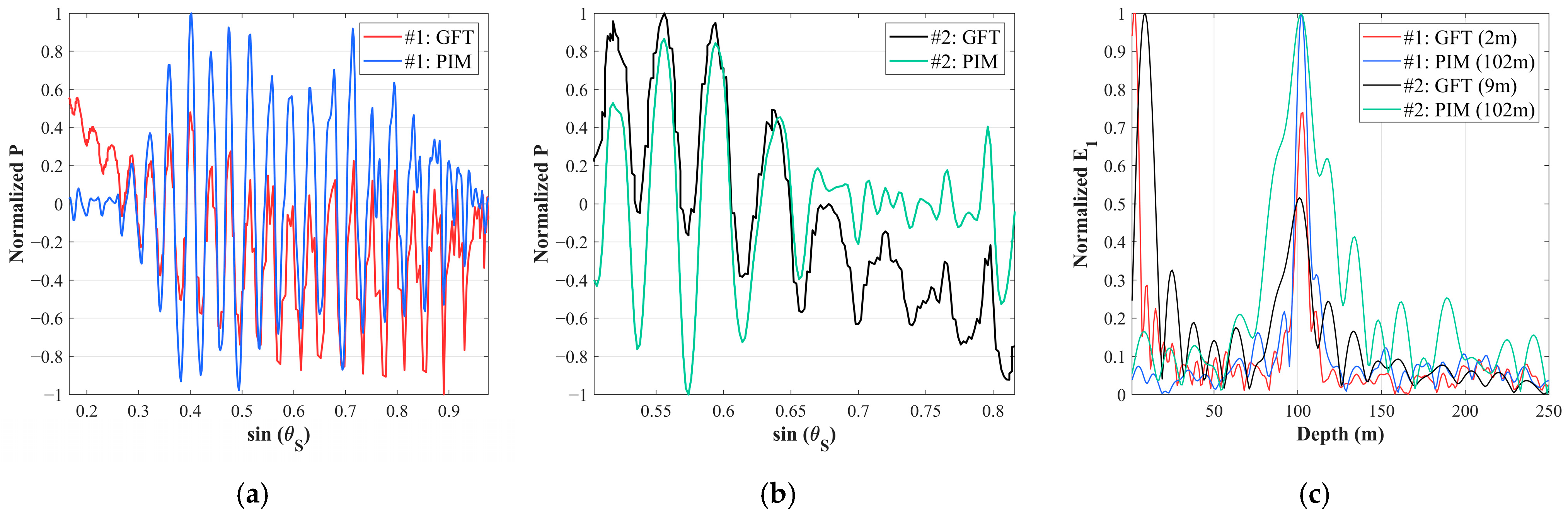
2.2. Generalized Fourier Transform

As analyzed in Section 2.1, the beamforming intensity along the interference trajectory is modulated by the product of source depth ( z s ) and grazing angle ( sin θ s ). For a moving source with the constant z s , there is a mapping relationship between the period of this sinusoidal modulation and the variable sin θ s . Therefore, this interference period in sinusoidal form can be estimated based on the Fourier transform:
F ( ω ) = f ( t ) e i ω t d t
It should be noted that Equation (3) is the general form of the Fourier transform (from the time domain to the frequency domain). For the interference trajectories on the VTR (Figure 1b), the beamforming intensity along which are converted from the grazing angle domain to the depth domain. As a generalized Fourier transform (GFT), by replacing t , ω , f , and F with sin θ t r , z , P and E1 respectively, the ambiguity function ( E 1 ) of the source depth can be expressed as follows [14,15]:
E 1 ( z ) = t r P sin θ t r ( t ) e i z sin θ t r ( t ) d sin θ t r ( t )
where t r ( ) represents the path integral formulation ( t r refers to the interference trajectory in Figure 1b). P and θ t r ( t ) are the beamforming intensity and the grazing angle at time t along t r , respectively.
Figure 2 shows the normalized beamforming intensity along trajectory #1 (red curve in Figure 2a) and #2 (black curve in Figure 2b). Due to the vertical directivity of deep-sea ambient noise as well as the variation in transmission loss during the source movements, the intensity decreases exponentially with the increase in grazing angle and is accompanied by periodic oscillation. Further, the depth ambiguity functions corresponding to the trajectories are calculated based on Equation (4), and there are significant peaks, seen in E 1 ( z ) , of two trajectories around the true depth ( z s = 100 m) of the source (red and black curves in Figure 2c). However, there is a higher peak in the range of z < 20 m and it is likely mistaken as a sea-surface source. This corresponds to the exponential downtrend as a low-frequency component.

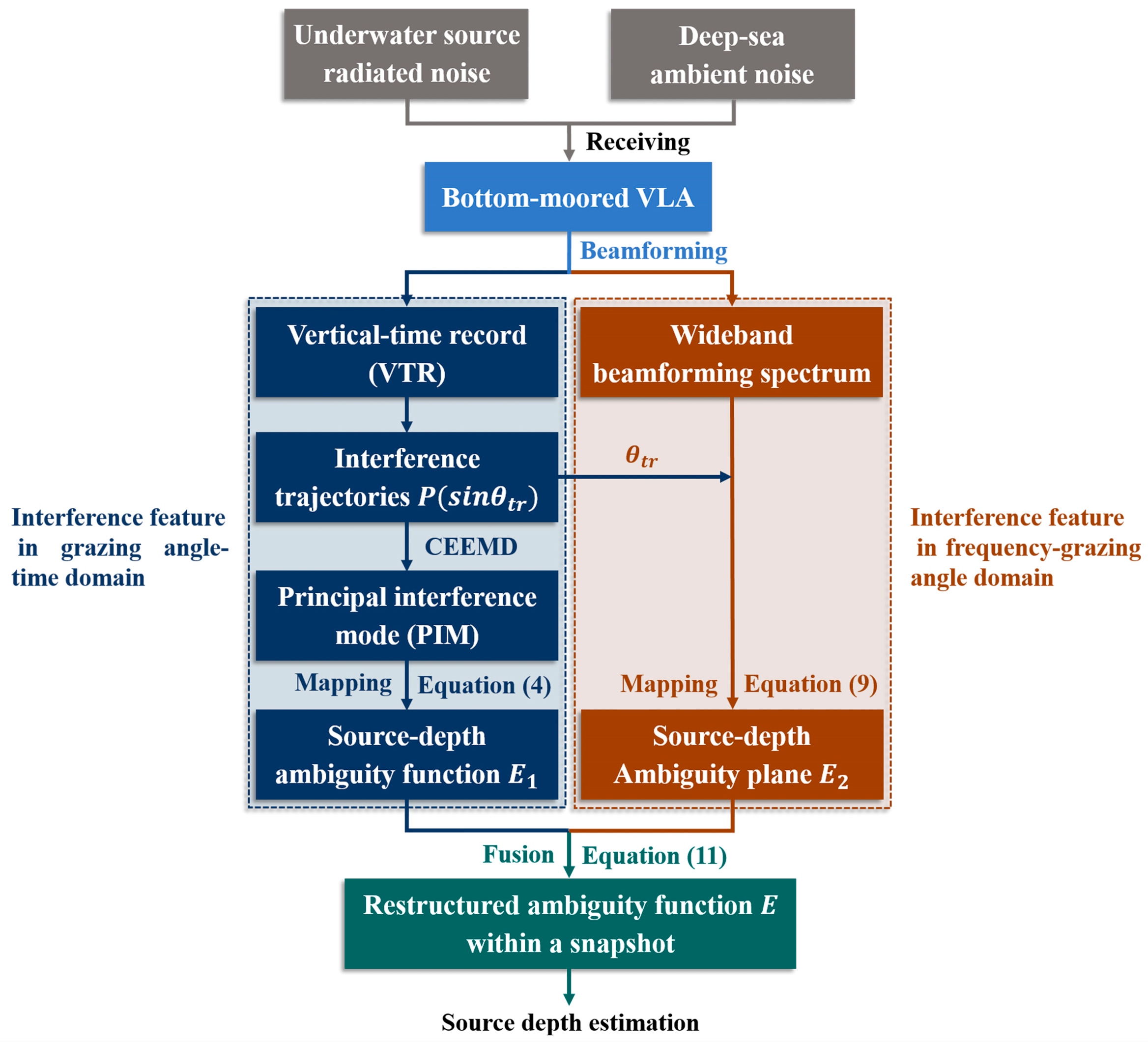
2.3. Interference Feature Fusion in Space–Time–Frequency Domain for Depth Estimation

The above simulation indicates that the interference pattern will be “destroyed” in the complex underwater acoustic environment (characterized by strong background noise and non-cooperative sources) and that the interference periods are not strictly modulated by the sine function, thus producing false peaks. Applying the GFT inevitably leads to a larger error in depth estimation. In addition, the formulation of the interference fringes in the VTR requires the source to transmit a single-frequency signal stably and the received signals need to be processed for a long period of time, limited application in real scenarios. Therefore, the interference characteristics of the wideband source in the frequency domain are also considered, and an interference feature fusion (IFF) method is proposed in the space–time–frequency domain for depth estimation to overcome the above limitations. The IFF method is described below.
To eliminate the false peaks, the complete-ensemble empirical mode decomposition (CEEMD) algorithm [27] is utilized to extract the principal interference mode from the non-linear and non-stationary beamforming intensity sequences. Before the decomposition, we add a pair of white Gaussian noises with opposite signs to the beamforming intensity sequence ( P ( sin θ t r ) ) along the interference trajectory, which can reduce the effects of the impulse signal in beamforming intensity sequence and improve the robustness of decomposition:
Y 1 n Y 2 n = 1 1 1 1 P ( sin θ t r ) W n
where W n is the noise added for the n -th time ( n = 1, 2, …, N ) with the standard deviation of σ W G N .
The empirical mode decomposition [28] is performed to decompose Y 1 n and Y 2 n to obtain their respective interference modes:
Y 1 n = q = 1 Q I M 1 , q n + R E 1 n Y 2 n = q = 1 Q I M 2 , q n + R E 2 n
where I M 1 , q n and I M 2 , q n are the q -th interference mode, and Q is the total modal number. R E 1 n and R E 2 n denote the residual terms, respectively.
Further, the mean value of the q -th interference mode with different periods is calculated using Equation (7), and the principal interference mode (PIM) can be extracted based on Equation (8):
I M q = 1 N n = 1 N I M 1 , q n + I M 2 , q n 2
P I M = arg max σ q 2 σ P 2
where σ q 2 and σ P 2 represent the variances in I M q and P ( sin θ t r ) , respectively.
On the basis of Equation (8), the ambiguity function of the source depth is updated by replacing P ( sin θ t r ) in Equation (4) with P I M . Figure 2a,b shows that the beamforming intensity sequence of the GFT shows the periodic oscillation (at a high frequency) accompanied by an exponential downward trend (at a low frequency), which causes interference mode aliasing. The PIM can better reflect the high-frequency interference period of the beamforming intensity sequences (Figure 2a,b) and eliminate the false peaks of E 1 ( z ) as to obtain accurate depth estimation results for underwater sources (Blue and green curves in Figure 2c).
For the wideband sources, there are also interference features present in the wideband beamforming output maps as a function of vertical arrival angle and frequency (i.e., in frequency–grazing angle domain). Similar to Equation (4), by replacing t , ω and F in Equation (3) with f , z sin θ S and E 2 , respectively, the wideband beamforming spectrum can be further mapped to the depth–grazing angle domain and the ambiguity plane ( E 2 ) of the source depth is constructed as follows:
E 2 t , sin ( θ S ) , z = f P t , sin ( θ S ) , f e i f z sin ( θ S ) d f
where P t , sin ( θ S ) , f represents the wideband beamforming spectrum at time t .
In addition, the critical condition of Equation (9) is determined as follows:
z c 0 B sin ( θ S )
where B and c 0 are bandwidth and average sound speed of seawater, respectively.
Figure 3a shows the wideband beamforming spectrum at t = 70 min during the source movement in Figure 1b. It can be seen that the distant shipping noise (black rectangle in Figure 3a) almost covers all frequency bands and its amplitude is highees in the low-frequency band ( f < 150 Hz). In addition, the beamforming intensity (as a function of frequency) at sin ( θ S ) = 0.67 also appears as an interference fringe that is related to the source depth. As can be seen from the depth ambiguity plane (Figure 3b), although there are “bright areas” (false peaks) on the ambiguity plane ( E 2 ) when sin ( θ S ) < 0.25, there are also “bright spots” in the position of sin ( θ S ) = 0.67 and z = 100 m (red circle in Figure 3b), corresponding to the true source position.
Based on the depth ambiguity function E 1 and plane E 2 , transformed from the VTR and the wideband beamforming spectrum, respectively, a new ambiguity function is constructed using the IFF and the source depth can be estimated in real time within a sliding time window. The entire implementation process of the IFF is described as follows:
Firstly, the beamforming intensity sequence along the interference trajectory on the VTR within the time interval [ t 1 , t n ] is taken as a snapshot, and CEEMD is performed to extract the principal interference mode of the snapshot data. Subsequently, the ambiguity function ( E 1 ( t n , z ) ) of the source depth (white dashed line in Figure 4a) within a snapshot is converted using Equation (4).
In addition, the wideband beamforming spectrum at each discrete time instant ( t i ) within the time interval [ t 1 , t n ] is mapped to the ambiguity plane ( E 2 t i , sin ( θ S ) , z ) of the source depth by utilizing Equation (9), as shown in Figure 4b–d.
Furthermore, for each time instant ( t i ), the sequence E 2 t i , sin θ S ( t i ) , z corresponding to the grazing angle of the trajectory on the VTR (white dashed lines in Figure 4b–d) is extracted and plugged into Equation (11), and the depth ambiguity function obtained by the fusion of interference features in space–time–frequency domain can be expressed as follows:
E ( t n , z ) = E 1 ( t n , z ) i = 1 n E 2 t i , sin θ S ( t i ) , z
where E 2 t i , sin θ S ( t i ) , z is normalized by scaling between 0 and 1. E ( t n , z ) is the newly constructed ambiguity function of source depth, and the z corresponding to maximum E ( t n , z ) is the estimated value of source depth at time t n .
Lastly, the sliding window-based processing method is applied to the whole beamforming intensity sequence along the interference trajectory on the VTR. By conducting the above steps for each snapshot (the sliding window size is determined as T w i n ), source depth estimation can be carried out continuously and in real time. The overall implementation process of the IFF is summarized in Figure 5.

3. Simulation and Analysis

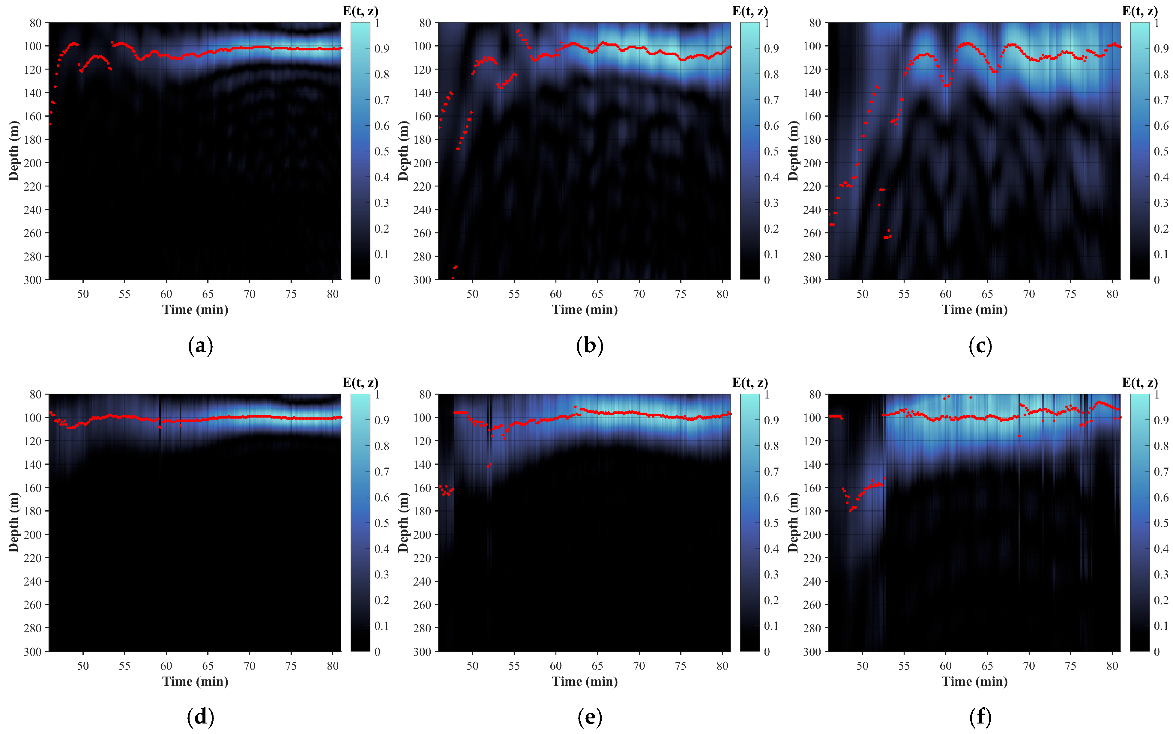
3.1. Depth Estimation for Single Source

It should be noted that the IFF method contains two hyperparameters that directly affect the accuracy of the IFF. These are the standard deviation of the noise ( σ W G N ) during the CEEMD process and the sliding window size ( T w i n ). Therefore, the sensitivity analysis experiment is carried out for the determination of the optimal parameter combination. As shown in Figure 6a, the average depth estimation error ( μ e ) of the IFF is relatively large ( μ e > 20 m) for T w i n < 5 min and increases with the rising σ W G N . The estimation errors are generally small ( μ e ~10 m) and insensitive to the change in both hyperparameters. Moreover, it can be seen from Figure 6b that the computation time ( T c a l ) of the IFF is inversely proportional to T w i n and less than 300 ms, which is acceptable in engineering implementation. Therefore, within the acceptable range of the estimation error, the IFF with a short T w i n has better real-time processing ability and lower estimation error for sources with rapidly changing depths. Based on the sensitivity analysis result, the optimal hyperparameter combination of σ W G N = 0.7 and T w i n = 12 min (corresponding to the minimum μ e ) is adopted in the subsequent simulation.
Based on the above results, the GFT and IFF methods are applied to the single-source scene for comparison and analysis. The ocean basin with a depth of 4000 m is taken as the research area in this study. Additionally, the seabed topography is assumed to be flat and the acoustic field is isotropic in the horizontal direction. The hydrologic data comes from the global Hybrid Coordinate Ocean Model (HYCOM) reanalysis with the Navy Coupled Ocean Data Assimilation [29] and the sound speed profile is shown in Figure 7a. Since the major noise sources of the typical underwater robots (e.g., manned submersibles and the unmanned underwater vehicles) include the low-frequency mechanical noise (wideband random signals) and the propeller noise (harmonic signals), the radiation noise spectrum of the underwater robots is modeled as the superposition of the wideband continuous spectrum (<1 kHz) as well as the discrete line spectrum [30,31]. Furthermore, considering the characteristics of the noise field in actual deep ocean, including the near-field wind-driven and far-field distant shipping noise [32], the frequency and spatial distribution characteristics of the noise field are also taken into account in the simulation of the ambient noise.
Firstly, the closest point of approach (CPA) from source to the VLA (Figure 7b) is considered, and the GFT and IFF methods are utilized to estimate the source depth continuously with a sliding window. Figure 8 shows the ambiguity plane of the source depth obtained by two methods, and it can be seen that the sidelobes of the ambiguity plane obtained by IFF are lower than that of the GFT on the whole. During the source movement for 45 min < t < 55 min (when the source has just entered the direct arrival zone), the depth estimation error of the GFT increases significantly (with a maximal error ofmore than 100 m) as the length of interference trajectory is too short (Figure 8a,b), while the estimate of the IFF can converge to the true depth of the source faster with a lower error (Figure 8d,e). In addition, the accuracy of both two estimation methods decreases when CPA increases to 9 km with the increase in the interference period within the same time window, while the IFF (with average estimation error μ e = 11.2 m) is superior to the GFT ( μ e = 33.2 m) (Figure 8c,f).
Based on Figure 8, the GFT and IFF are tested and compared under different signal-to-noise ratio (SNRs), respectively. Figure 9 shows that the depth estimation errors of both methods decrease exponentially with the increase in the SNR. For SNR > −9 dB, both methods can achieve relatively high estimate accuracy ( μ e < 10 m), and the average estimation error of the IFF is reduced by ~55% compared with GFT. Moreover, the μ e of the IFF is ~63% lower than that of the GFT for SNR < −9 dB, although the estimation errors increase significantly. It is difficult for both methods to obtain relatively accurate estimation results with the further reduction in the SNR for the distant shipping noise completely covered the interference fringes produced by the source. In general, the IFF is significantly superior to the GFT under different SNRs.
In addition, the performance of the methods for depth estimation with different source depths ( z s ) is further analyzed. As shown in Figure 10, the depth estimation errors of the GFT and IFF methods decrease slightly with the increase in z s for z s < 220 m. On the contrary, the depth estimation errors of two methods increase exponentially when z s > 220 m due to the large difference in grazing angles between the D and the SR arrivals, resulting in a separation/bifurcation of the interference fringes of two arrival paths on the VTR (without complete coherent superposition and forming a clear and intact interference pattern). Overall, the depth estimation errors of the IFF are reduced by ~47% on average compared to GFT.

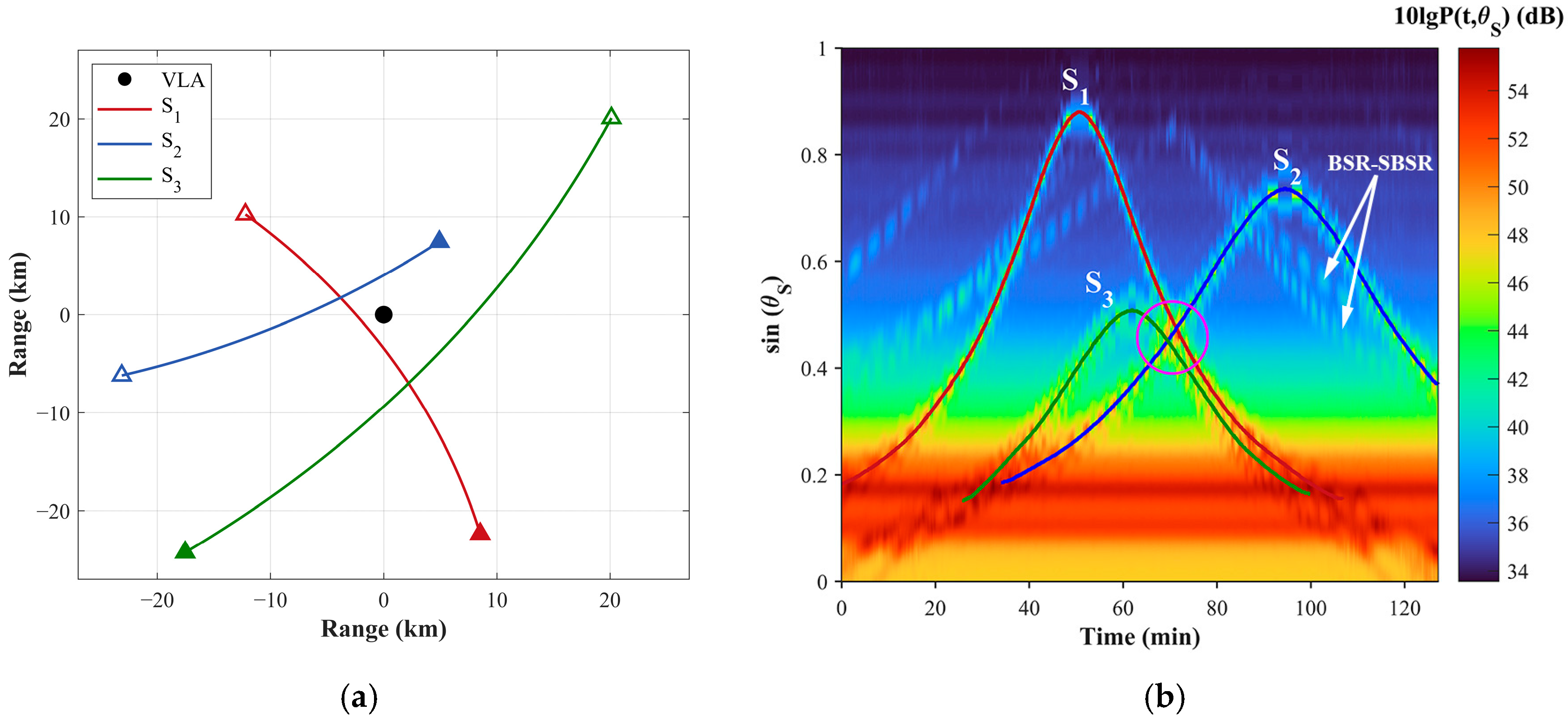
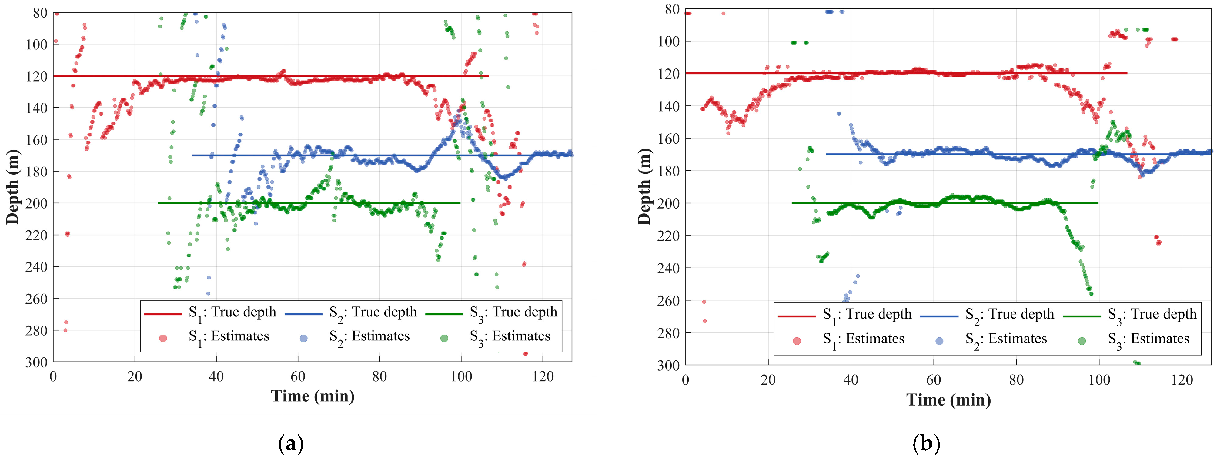
3.2. Depth Estimation for Multiple Sources

Further, the GFT and IFF are tested for depth separation in the multi-source scenario. Figure 11a shows the trajectories of three underwater sources with different depths and a constant turn motion in the horizontal plane, and the detailed parameters of each source are shown in Table 1 (modeling of the source-radiated noise is the same as that in Section 2.1). The continuous estimation results of multiple sources obtained by both methods are displayed in Figure 12, and it can be seen that the interference structures are masked by distant shipping noise (Figure 11b) when each source is far away from the VLA (corresponding to the small vertical arrival angle with sin ( θ S ) < 0.3 ), resulting in a large deviation in the source depth estimation of the GFT (Figure 12a), especially for source S3 with t < 40 min. Within the period of 60 min < t < 80 min, the depth estimation error of the GFT gradually increases for S3, while the IFF can still accurately separate the depth of multiple sources (with lower estimation error) even though the interference tracks of sources are across each other on the VTR (magenta circle in Figure 11b). In addition, the D-SR interference pattern of source S2 was in a coherent superposition with the BSR-SBSR interference pattern of sources S1 (red curve) and S3 (green curve) and its original interference structure was disrupted, which increased the estimation error of both methods. The IFF can still separate S1 and S2 around t = 100 min (Figure 12b), and its average estimation error for S1, S2 and S3 decreases by 24%, 29% and 37% compared with GFT, respectively. The depth estimation results for multiple sources with variable depth (Figure 13) also indicated that the IFF can separate the depths of complexly and highly maneuvering sources effectively, with the average estimation error reduced by 23% compared with GFT.

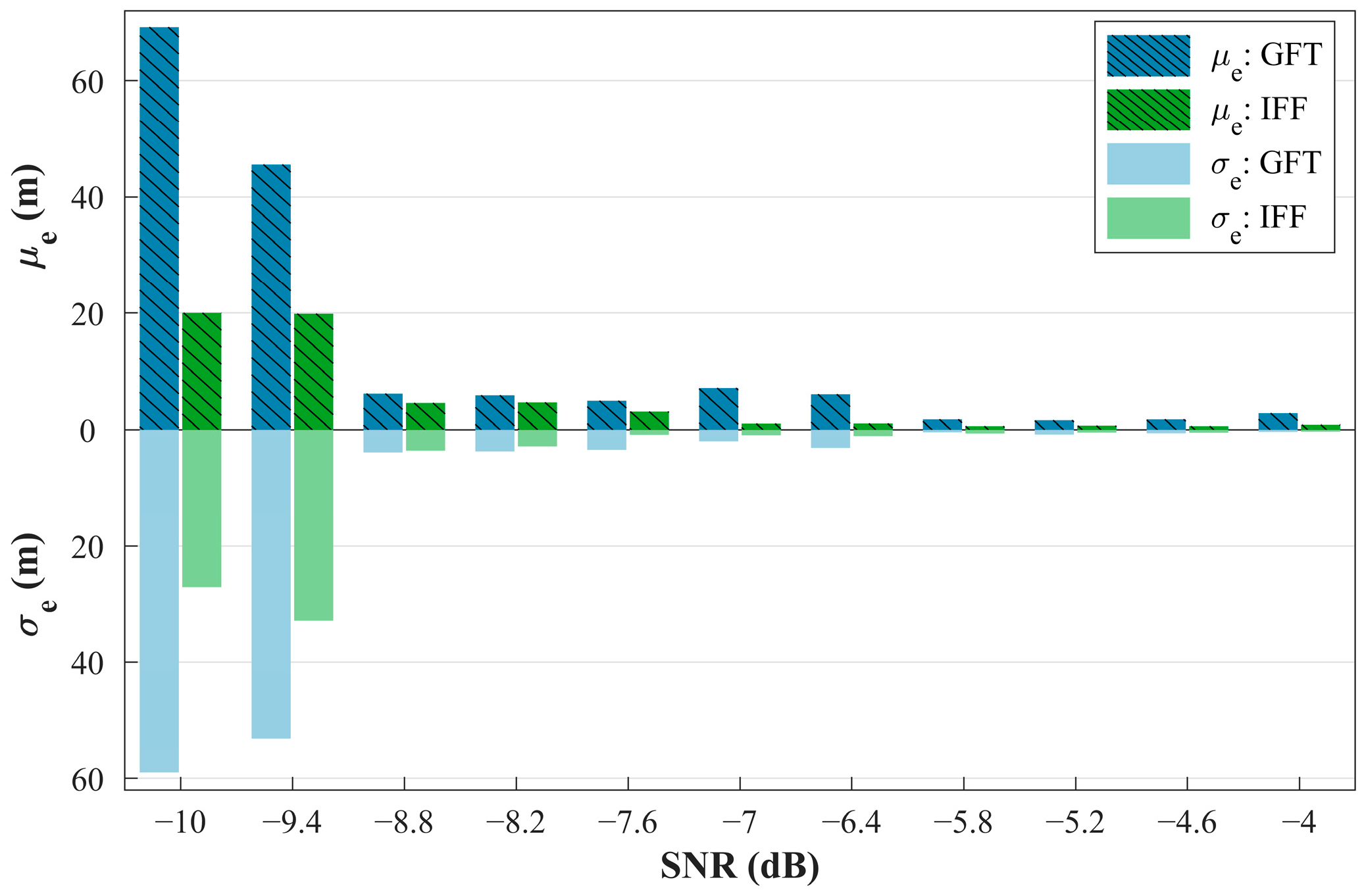
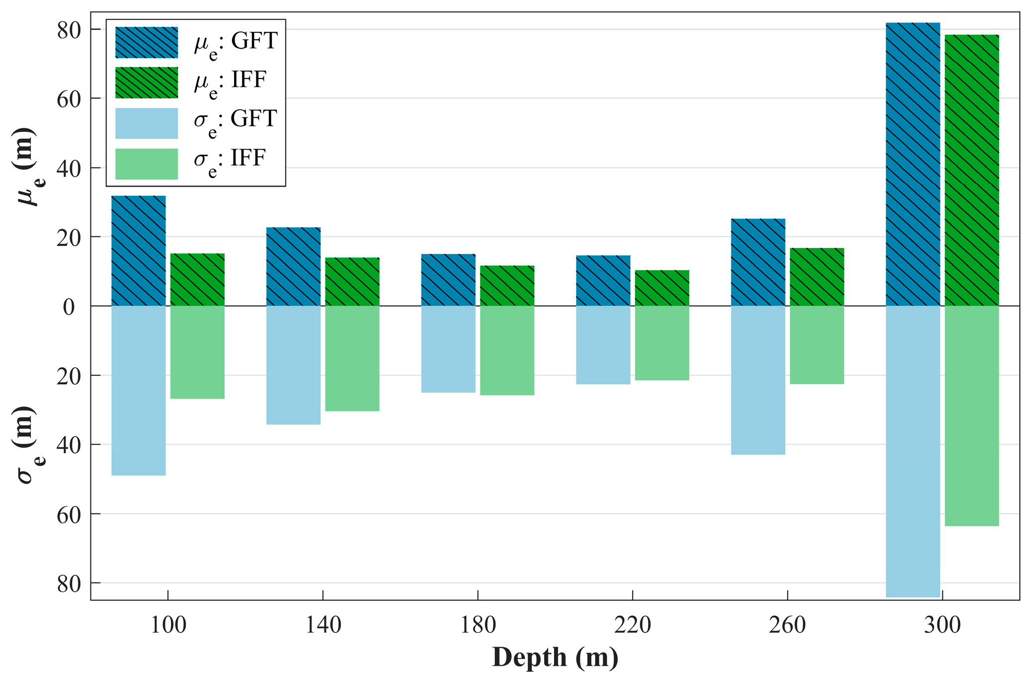
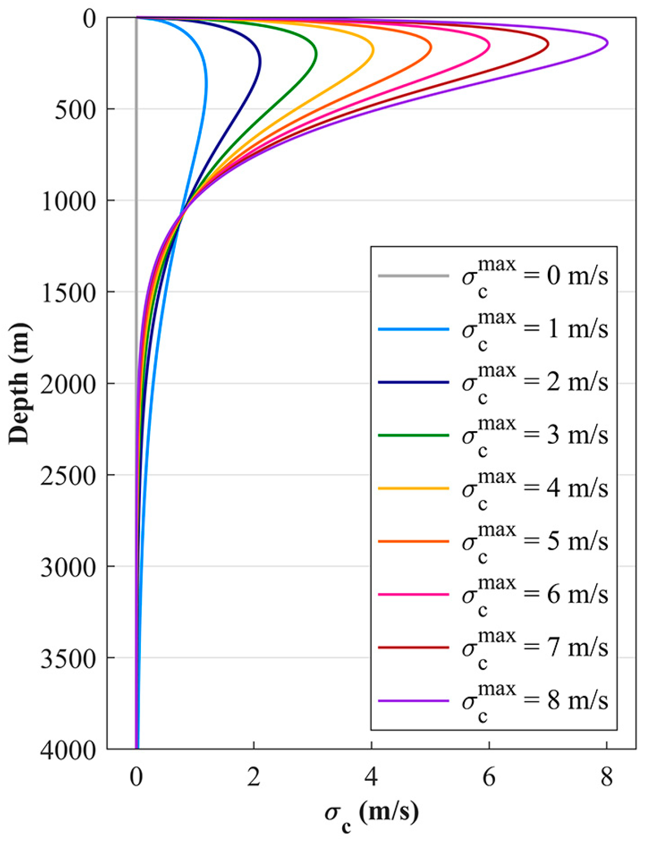
3.3. Robustness Analysis

In the real ocean, the spatial and temporal changes in the underwater acoustic channel are complex, and the hydrological conditions change over time due to marine dynamic processes such as internal waves and tides in the same sea area. The uncertainty of the environment can cause the fluctuation of the sound velocity in seawater and affect the characteristics of the acoustic field [26,33]. Therefore, the robustness of the IFF under dynamic and fluctuating sound speed profiles is simulated and analyzed in this section.
In the typical deep-sea environment, the fluctuation of the sound velocity near the sea surface is sharp. Thus, is mostly influenced by diurnal variation, wind waves, and swells. The sound velocity below the surface mixed layer decreases with the increase in depth, and is relatively stable and almost unchanged below the SOFAR channel [34]. Based on these characteristics, sound speed profiles ( c ) with different fluctuation degrees are constructed according to Equation (12), and the standard deviations ( σ c ) of sound velocity at different depths (with maximum value σ c max ) is shown in Figure 14.
c ( z ) = c 0 ( z ) + 3 σ c ( z ) U ^ ( 0 , 1 )
where c 0 ( z ) is the original sound speed profile (Figure 7a), and U ^ ( 0 , 1 ) represents the random numbers uniformly distributed in the interval [0, 1].
Figure 15 shows the depth estimation errors of the GFT and IFF for a single source (the source motion state is the same as that in Figure 1b) at different σ c max . It can be seen from Figure 15a that the depth estimation error of both methods is low and acceptable for σ c max < 3 m/s, and the average estimation error of the IFF is reduced by 12% compared with GFT. However, the propagation time delay between the D and SR paths fluctuates greatly for σ c max > 3 m/s due to the drastic fluctuation of the acoustic channel. As a result, the interference period of the reconstructed PIM gradually deviates from the theoretical value (0.04) under the isovelocity assumption, which results in a continued increase in the depth estimation error (Figure 15b).

4. Conclusions and Discussion

This paper introduces a depth estimation and separation method for underwater robots based on the interference feature fusion (IFF) in the deep sea. By performing CEEMD on the beamforming intensity along the interference trajectory in the grazing angle–time domain (VTR), the IFF can extract the principal interference mode adaptively and eliminate the low-frequency components (false peaks) generated by traditional GFT-based methods due to the spatial directivity of the distant shipping noise. Further, the IFF also fuses the interference feature of the source in frequency–grazing angle domain and further improves the depth estimation accuracy without the need for data accumulation over a long period of time. The theoretical analysis and simulation experiments show that the estimation error of the IFF under multiple conditions is significantly reduced (>28%) compared with GFT in the case of completely unknown environmental information. Additionally, the sensitivity/robustness analysis indicate that the IFF has a low computational complexity (<300 ms for computing time) and exhibits a high degree of environmental robustness for σ c max < 3 m/s ( σ c max denotes the maximum standard deviation of sound speed fluctuations). The proposed method can be applied to the vertical line array deployed in the direct-arrival zone to realize the long-term continuous depth estimation of the underwater sources and establish the foundation for the subsequent state inspection and tracking of underwater robots.
It is worth noting that the IFF is proposed based on the assumption that the radiated noise of underwater source is a wideband signal, which is limited by the processing bandwidth gain and the characteristics of the source-radiated noise. For a narrowband source, since the IFF struggles to fuse the interference features in the frequency–grazing angle domain, a longer period of received data accumulation is required to obtain accurate estimation, although the real-time processing performance will also be degraded substantially. In addition, the arrival angle of the underwater source decreases exponentially with the increase in its distance within the deep-sea acoustic channel. For medium-distance sources with small arrival angles, its interference structure will be obscured by the distant shipping noise, leading to an increase in the passive depth estimation error due to the low SNR. Therefore, the suppression of the distant shipping noise and the feature enhancement of the interference pattern will be the focus of follow-up research.

Author Contributions

Methodology and writing—original draft preparation, L.R.; conceptualization, writing—review and editing and project administration, B.L.; validation, T.G.; data curation, Z.H. All authors have read and agreed to the published version of the manuscript.

Funding

This research was funded by the National Natural Science Foundation of China (12174311), Natural Science Basic Research Program of Shaanxi (2023-JC-JQ-07) and Key R&D Program of Shandong Province, China (2023CXPT051).

Data Availability Statement

The data presented in this study are available on request from the corresponding author.

Conflicts of Interest

The authors declare no conflicts of interest.

Abbreviations

The following abbreviations are used in this study:
VTRvertical-time record
IFFinterference feature fusion
RAPreliable acoustic path
SNRsignal-to-noise ratio
VLAvertical line array
GFTgeneralized Fourier transform
D-pathdirect path
SR-pathsurface-reflected path
MVDRMinimum Variance Distortionless Response
BSRbottom–surface-reflected
SBSRsurface–bottom–surface-reflected
CEEMDcomplete-ensemble empirical mode decomposition
PIMprincipal interference mode
HYCOMhybrid coordinate ocean model
CPAclosest point of approach
SOFARsound fixing and ranging

References

  1. Qiu, C.; Ma, S.; Chen, Y.; Meng, Z.; Wang, J. Reliable acoustic path and directed-arrival zone spatial gain analysis for a vertical line array. Sensors 2018, 18, 3462. [Google Scholar] [CrossRef] [PubMed]
  2. Liu, Y.; Chen, C.; Feng, X. Investigating the reliable acoustic path properties in a global scale. Front. Mar. Sci. 2023, 10, 1213002. [Google Scholar] [CrossRef]
  3. Sun, M.; Zhou, S. Complex acoustic intensity with deep receiver in the direct-arrival zone in deep water and sound-ray-arrival-angle estimation. Acta Phys Sin. 2016, 65, 164302. [Google Scholar] [CrossRef]
  4. Li, Z.; Zurk, L.M.; Ma, B. Vertical arrival structure of shipping noise in deep water channels. In Proceedings of the OCEANS 2010 MTS/IEEE SEATTLE, Seattle, WA, USA, 20–23 September 2010; pp. 1–8. [Google Scholar] [CrossRef]
  5. Qiu, C.; Chen, Y.; Ma, S.; Meng, Z. Spatial gain analysis for vertical linear array in the direct-arrival zone. In Proceedings of the 2018 IEEE International Conference on Signal Processing, Communications and Computing (ICSPCC), Qingdao, China, 14–16 September 2018; pp. 1–5. [Google Scholar] [CrossRef]
  6. Lei, Z.; Yang, K.; Ma, Y. Passive localization in the deep ocean based on cross-correlation function matching. J. Acoust. Soc. Am. 2016, 139, EL196–EL201. [Google Scholar] [CrossRef]
  7. Cao, R.; Yang, K.; Yang, Q.; Chen, P.; Sun, Q.; Xue, R. Localization of two sound sources based on compressed matched field processing with a short hydrophone array in the deep ocean. Sensors 2019, 19, 3810. [Google Scholar] [CrossRef] [PubMed]
  8. Liu, W.; Yang, Y.; Lü, L.; Shi, Y.; Liu, Z. Source localization by matching sound intensity with a vertical array in the deep ocean. J. Acoust. Soc. Am. 2019, 146, EL477–EL481. [Google Scholar] [CrossRef]
  9. Geroski, D.J.; Dowling, D.R. Robust long-range source localization in the deep ocean using phase-only matched autoproduct processing. J. Acoust. Soc. Am. 2021, 150, 171–182. [Google Scholar] [CrossRef]
  10. Shang, E.; Wang, Y. Environmental mismatching effects on source localization processing in mode space. J. Acoust. Soc. Am. 1991, 89, 2285–2290. [Google Scholar] [CrossRef]
  11. Le Gall, Y.; Dosso, S.E.; Socheleau, F.X.; Bonnel, J. Bayesian source localization with uncertain Green’s function in an uncertain shallow water ocean. J. Acoust. Soc. Am. 2016, 139, 993–1004. [Google Scholar] [CrossRef]
  12. Tran, J.M.Q.; Hodgkiss, W.S. Matched-field processing of 200-Hz continuous wave (cw) signals. J. Acoust. Soc. Am. 1991, 89, 745–755. [Google Scholar] [CrossRef]
  13. Weng, J.; Yang, Y. A passive source range and depth estimation method by single hydrophone in shadow zone of deep water. Acta Acust. 2018, 43, 905–914. [Google Scholar] [CrossRef]
  14. McCargar, R.; Zurk, L.M. Depth-based signal separation with vertical line arrays in the deep ocean. J. Acoust. Soc. Am. 2013, 133, EL320–EL325. [Google Scholar] [CrossRef]
  15. Zurk, L.M.; Boyle, J.K.; Shibley, J. Depth-based passive tracking of submerged sources in the deep ocean using a vertical line array. In Proceedings of the 2013 Asilomar Conference on Signals, Systems and Computers, Pacific Grove, CA, USA, 3–6 November 2013; pp. 2130–2132. [Google Scholar] [CrossRef]
  16. Kniffin, G.P.; Boyle, J.K.; Zurk, L.M.; Siderius, M. Performance metrics for depth-based signal separation using deep vertical line arrays. J. Acoust. Soc. Am. 2016, 139, 418–425. [Google Scholar] [CrossRef]
  17. Zhu, F.; Zheng, G.; Liu, F. A matched beam intensity processing method for estimating source depth using vertical linear array in deep water. In Proceedings of the 2021 OES China Ocean Acoustics (COA), Harbin, China, 14–17 July 2021; pp. 894–899. [Google Scholar] [CrossRef]
  18. Duan, R.; Yang, K.; Li, H.; Ma, Y. Acoustic-intensity striations below the critical depth: Interpretation and modeling. J. Acoust. Soc. Am. 2017, 142, EL245–EL250. [Google Scholar] [CrossRef]
  19. Yang, K.; Xu, L.; Yang, Q.; Duan, R. Striation-based source depth estimation with a vertical line array in the deep ocean. J. Acoust. Soc. Am. 2018, 143, EL8–EL12. [Google Scholar] [CrossRef]
  20. Zheng, G.; Yang, T.C.; Ma, Q.; Du, S. Matched beam-intensity processing for a deep vertical line array. J. Acoust. Soc. Am. 2020, 148, 347–358. [Google Scholar] [CrossRef]
  21. Zhou, L.; Zheng, G.; Yang, T.C. Target depth estimation by frequency interference matching for a deep vertical array. Appl. Acoust. 2022, 186, 108493. [Google Scholar] [CrossRef]
  22. Qi, Y.; Zhou, S.; Liu, C. Sources depth estimation for a tonal source by matching the interference structure in the arrival angle domain. J. Acoust. Soc. Am. 2023, 154, 2800–2811. [Google Scholar] [CrossRef]
  23. Wu, Y.; Li, P.; Guo, W.; Zhang, B.; Hu, Z. Passive source depth estimation using beam intensity striations of a horizontal linear array in deep water. J. Acoust. Soc. Am. 2023, 154, 255–269. [Google Scholar] [CrossRef]
  24. Liu, Y.; Niu, H.; Li, Z.; Zhai, D.; Chen, D. Source depth estimation based on Gaussian processes using a deep vertical line array. Appl Acoust. 2024, 215, 109684. [Google Scholar] [CrossRef]
  25. Wang, W.; Wang, Z.; Su, L.; Hu, T.; Ren, Q.; Gerstoff, P.; Ma, L. Source depth estimation using spectral transformations and convolutional neural network in a deep-sea environment. J. Acoust. Soc. Am. 2020, 148, 3633–3644. [Google Scholar] [CrossRef]
  26. Jensen, F.B.; Kuperman, W.A.; Porter, M.B.; Schmidt, H.; Tolstoy, A. Computational Ocean Acoustics, 2nd ed.; Springer: New York, NY, USA, 2011; pp. 15–20. [Google Scholar]
  27. Yeh, J.R.; Shieh, J.S.; Huang, N.E. Complementary ensemble empirical mode decomposition: A novel noise enhanced data analysis method. Adv. Adapt. Data. Anal. 2010, 2, 135–156. [Google Scholar] [CrossRef]
  28. Huang, N.E.; Shen, Z.; Long, S.; Wu, M.; Shih, H.H.; Zheng, Q.A.; Nai-Chyuan, Y.; Tung, C.C.; Liu, H. The empirical mode decomposition and the Hilbert spectrum for nonlinear and non-stationary time series analysis. Proc. R. Soc. Lond. A 1998, 454, 903–995. [Google Scholar] [CrossRef]
  29. Chassignet, E.P.; Hurlburt, H.E.; Smedstad, O.M.; Halliwell, G.R.; Hogan, P.J.; Wallcraft, A.J.; Baraille, R.; Bleck, R. The HYCOM (hybrid coordinate ocean model) data assimilative system. J. Mar. Syst. 2007, 65, 60–83. [Google Scholar] [CrossRef]
  30. Yu, C.; Wang, R.; Zhang, X.; Li, Y. Experimental and numerical study on underwater radiated noise of AUV. Ocean. Eng. 2020, 201, 107111. [Google Scholar] [CrossRef]
  31. Liu, S.; Zhang, Q.; Shi, W. Self-noise characteristic analysis of a type of UUV. In Proceedings of the 2022 IEEE International Conference on Signal Processing, Communications and Computing (ICSPCC), Xi’an, China, 25–27 October 2022; pp. 1–6. [Google Scholar] [CrossRef]
  32. Yang, Q.; Yang, K.; Cao, R.; Duan, S. Spatial vertical directionality and correlation of low-frequency ambient noise in deep ocean direct-arrival zones. Sensors 2018, 18, 319. [Google Scholar] [CrossRef] [PubMed]
  33. Sha, L.; Nolte, L.W. Effects of environmental uncertainties on sonar detection performance prediction. J. Acoust. Soc. Am. 2005, 117, 1942–1953. [Google Scholar] [CrossRef]
  34. Zhang, L.; Liu, Y.; Liu, Y.; Chen, G.; Li, M. Modeling of time-varying characteristics of deep-sea sound velocity profile based on layered EOF. Coast. Eng. 2022, 41, 209–222. [Google Scholar] [CrossRef]
Figure 1. (a) Geometric diagram of interference of acoustic field in direct arrival zone and (b) VTR at z s = 100 m and v s = 12 kn (white curves represent interference trajectories formed by superposition of different wave arrivals).
Electronics 14 02228 g001
Figure 2. Normalized beamforming intensity sequences (as functions of grazing angle) along (a) trajectory #1 and (b) trajectory #2 in Figure 1b as well as corresponding (c) ambiguity function ( E 1 ( z ) ) of source depth obtained by the GFT (red and black curves) and the PIM (blue and green curves).
Electronics 14 02228 g002
Figure 3. (a) Wideband beamforming spectrum and (b) ambiguity plane ( E 2 ) of source depth at t = 70 min (white area represents inapplicability of depth estimation determined by Equation (10)).
Electronics 14 02228 g003
Figure 4. (a) Ambiguity plane ( E 1 ( t , z ) ) of source depth within time interval [ t 1 , t n ] converted from VTR and ambiguity plane ( E 2 t , sin ( θ S ) , z ) at time instant (b) t 1 , (c) t i and (d) t n transformed from wideband beamforming spectrum (white dashed line in each subgraph represents the depth ambiguity vector at a specific time or grazing angle).
Electronics 14 02228 g004
Figure 5. The implementation flowchart of the IFF.
Electronics 14 02228 g005
Figure 6. The mean values of (a) the depth estimation error ( μ e ) and (b) computation time ( T c a l ) of the IFF with different combinations of hyperparameters ( σ W G N and T w i n ) based on the scenario in Section 2.1 (the white rectangle in (a) represents the parameter combination corresponding to the minimum μ e ).
Electronics 14 02228 g006
Figure 7. (a) Sound speed profile. (b) Source trajectory with CPA of 3 km (red line), 6 km (green line), and 9 km (blue line). The hollow and solid triangles represent the starting and ending positions, respectively. The source moves uniformly in a straight line ( z s = 100 m, v s = 12 kn) close to the VLA (Black dot).
Electronics 14 02228 g007
Figure 8. Normalized ambiguity plane ( E ( t , z ) ) obtained by GFT and IFF with CPA of (a,d) 3 km, (b,e) 6 km, and (c,f) 9 km (with time interval of 10 s and processing frequency band of 100–200 Hz). The red dots in each subgraph represent the depth estimation results of two methods.
Electronics 14 02228 g008
Figure 9. Mean ( μ e ) and standard deviation ( σ e ) of depth estimation errors for source with different SNR obtained by GFT (blue bars) and IFF (green bars) methods based on 487 samples.
Electronics 14 02228 g009
Figure 10. The mean ( μ e ) and the standard deviation ( σ e ) of the depth estimation errors for source at different depth ( z s ) obtained by the GFT (blue bars) and the IFF (green bars) methods based on 487 samples (CPA = 5 km).
Electronics 14 02228 g010
Figure 11. (a) Trajectories of multiple underwater sources (the hollow and solid triangles represent the starting and ending positions) and position of the VLA (black dot). (b) The VTR in the multi-source scene (the red, blue and green lines represent the traces of the D-SR interference fringes of the sources S1, S2 and S3, respectively).
Electronics 14 02228 g011
Figure 12. True depth (solid lines) and estimation results (dots) obtained by (a) GFT and (b) IFF during the movements of the sources S1 (red), S2 (blue) and S3 (green) with constant depth.
Electronics 14 02228 g012
Figure 13. True depth (solid lines) and the estimation results (dots) obtained by the (a) GFT and (b) IFF during the movements of the sources S1 (red), S2 (blue), and S3 (green) with variable depth (the horizontal tracks of sources are the same as those in Figure 11a).
Electronics 14 02228 g013
Figure 14. Profile of standard deviation ( σ c ) of sound velocity with different σ c max .
Electronics 14 02228 g014
Figure 15. (a) The mean ( μ e ) and the standard deviation ( σ e ) of the depth estimation errors for sources at different σ c max obtained by the GFT (blue bars) and the IFF (green bars) methods based on 487 samples. (b) The interference periods ( Δ ( sin θ S ) ) of the principal interference mode (PIM) at different σ c max and the theoretical value under the isovelocity assumption.
Electronics 14 02228 g015
Table 1. Detailed motion parameters of each source in Figure 11a.
SourceDepth (m)CPA (km)Speed (km)
S11201.9610
S21703.438
S32006.2415
Disclaimer/Publisher’s Note: The statements, opinions and data contained in all publications are solely those of the individual author(s) and contributor(s) and not of MDPI and/or the editor(s). MDPI and/or the editor(s) disclaim responsibility for any injury to people or property resulting from any ideas, methods, instructions or products referred to in the content.

