A Novel Image Encryption Scheme Based on a Quantum Logistic Map, Hyper-Chaotic Lorenz Map, and DNA Dynamic Encoding

Abstract

In the digital information age, although digital images are widely used, the security issues associated with them have become increasingly severe. Consequently, ensuring secure image transmission has become a critical challenge in contemporary information security research. Chaotic systems are characterized by non-periodic behavior, strong dependence on initial conditions, and other favorable characteristics, and have been widely employed in the scrambling and diffusion processes of image encryption. Compared to classical chaotic maps, a quantum Logistic map exhibits better randomness and stronger sensitivity to initial values, effectively overcoming the attractor problem inherent in classical Logistic maps, thereby significantly enhancing the robustness of encryption methodologies. This article focuses on a innovative integration of a quantum Logistic map, hyper-chaotic Lorenz map, and DNA dynamic encoding technology, to design and implement a highly secure and efficient image encryption scheme. First, high-quality random number sequences are produced utilizing the quantum Logistic map, which is then employed to perform a scrambling operation on the image. Next, by integrating the chaotic sequences yielded from the hyper-chaotic Lorenz map with DNA dynamic encoding and operation rules, we implement a diffusion process, thereby increasing the strength of the image encryption. Experimental simulation results and multiple security analyses demonstrated that our encryption methodology achieved excellent encryption performance, effectively resisting a variety of attack strategies, and it holds significant potential for research on protecting image information through encryption.

1. Introduction

As network and multimedia technologies develop rapidly, the quantity of images transmitted over networks has grown explosively. Nonetheless, the characteristic of network openness has made the security of image information an increasingly critical issue. Unlike text data, the high redundancy and strong correlation of pixels in images lead to problems such as slow encryption speeds and low efficiency in traditional encryption methods [1,2,3,4,5]. As a result, to ensure the security of image information, many researchers have devoted themselves to the study and development of efficient encryption algorithms tailored to the specific characteristics of images [6,7,8,9,10]. Among various algorithms, chaotic maps, because of their remarkable features, including sensitivity to starting parameters, non-periodicity, randomness, and unpredictability, offer high security and ease of implementation for encryption algorithms. Therefore, in the past few years, chaotic-map-based image encryption methods have drawn significant interest [11,12,13].

In 2014, Zhou et al. [14] put forward an image encryption algorithm which incorporates three chaotic maps: Logistic-Tent, Logistic-Sine, and Tent-Sine. When compared with an individual one-dimensional chaotic map, the sequence produced by combining multiple one-dimensional chaotic maps exhibited greater randomness. However, one-dimensional chaotic maps have various disadvantages, for example, short periods, small key spaces, low security, and suboptimal encryption performance [15,16]. In contrast, encryption algorithms built upon chaotic maps with high-dimensionality have garnered widespread attention due to their larger key spaces, strong sensitivity to initial conditions, and higher complexity of generated random sequences [17,18,19,20]. Nevertheless, image encryption algorithms designed using high-dimensional chaotic maps still face challenges, including insufficient chaotic characteristics, long processing times, and the increasing sophistication of decryption methods targeting chaotic techniques. To mitigate these risks, researchers have sought to introduce new technologies, such as neural networks [21,22], deep learning [23], artificial intelligence [24], and quantum computing [25], for the design of more secure, efficient, and flexible encryption algorithms and to address the increasingly complex network environment and advanced attack strategies.

DNA cryptography, as an emerging field, has gradually gained widespread attention. Its origins can be traced back to Adleman’s [26] exploration of the feasibility of DNA computing, which introduced biological elements into the field of information security. The enormous parallel processing ability, vast storage capacity, and extremely low power consumption of DNA sequences have prompted researchers to leverage DNA technology for the evolution of unique information security systems. Among these, image encryption schemes leveraging chaotic dynamics and DNA-inspired encoding strategies have become the subject of intense scholarly interest. In 2015, Li et al. [27] created a cryptographic technique for two images that makes use of DNA subsequence operations and chaotic maps. They utilized Lorenz and Chen maps to generate chaotic sequences that were used for image encryption by converting them into DNA matrices based on selected DNA coding rules. In that same year, Wu et al. [28] introduced an encryption technique for color images utilizing DNA-based sequences and multiple optimized one-dimensional chaotic maps. This scheme achieved encryption through DNA operations and random shuffling. However, the use of a single DNA encoding and operation rule strategy, or relying solely on low-dimensional chaotic maps for encryption, often leads to security vulnerabilities in the encryption structure and results in lower complexity. In 2021, Cun et al. [29] combined a new chaotic map boasting a elevated Lyapunov exponent and improved dynamic behavior with dynamic DNA encoding, enhancing the application prospects of dynamic DNA encoding within the scope of image encryption.

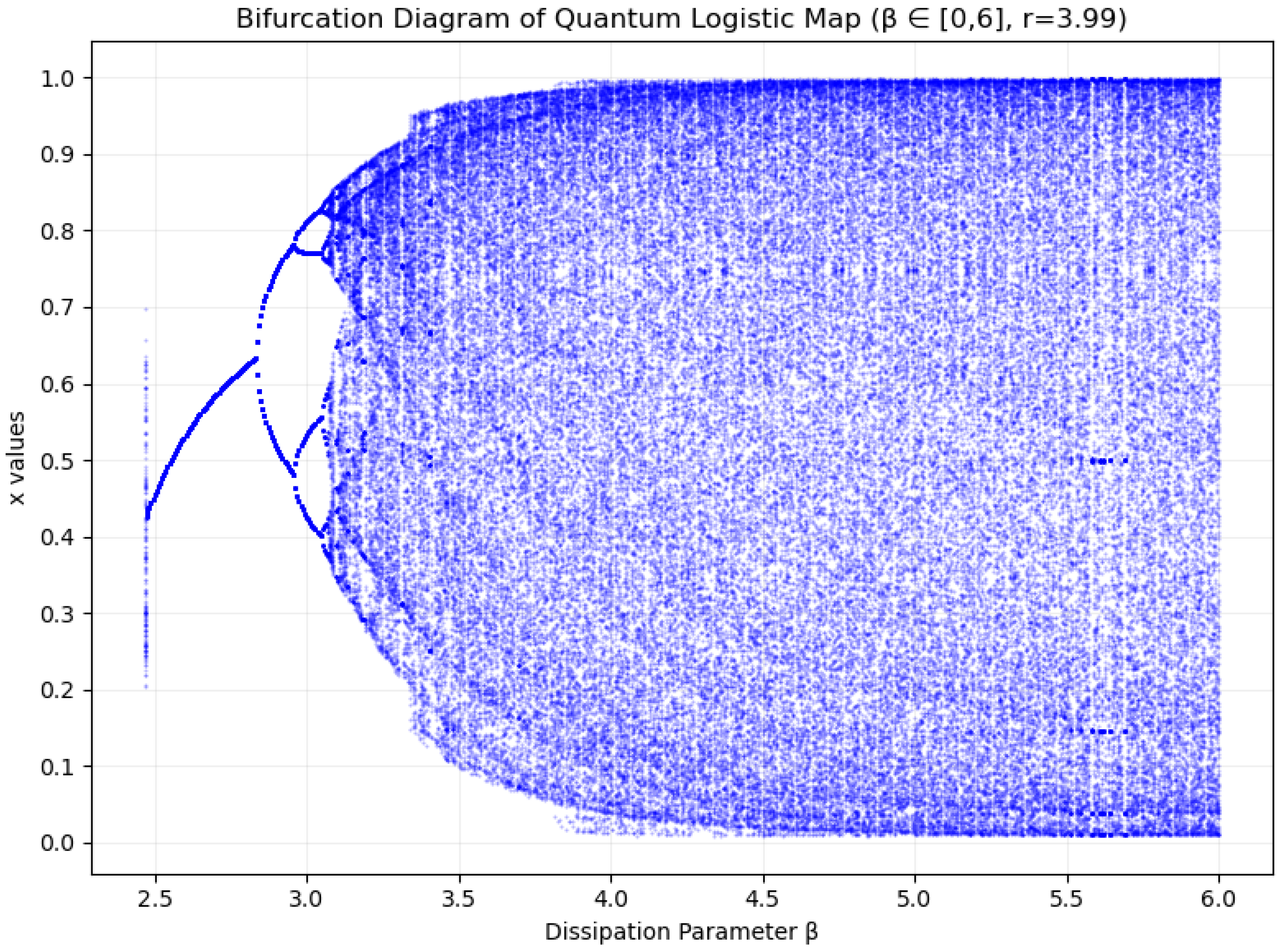
In recent years, quantum algorithms [30,31] have drawn extensive attention in the communication and processing domains. Compared with classical algorithms, they possess remarkable advantages regarding speed and security aspects. Notably, quantum chaos has shown great potential in the image processing field. The so-called quantum chaos is essentially the quantization of classical chaotic maps. In general, quantum maps fall into two categories: one involves the quantization of nonautonomous maps featuring a periodic time dependence, while the other concerns the quantization of abstract dynamical maps [32]. Akhshani et al. [32] were the first to propose an image encryption framework incorporating principles of a higher-complexity quantum chaotic map. They utilized the remarkable sensitivity of quantum chaos to subtle differences in starting conditions and regulatory parameters, thereby augmenting the security of the algorithm. Subsequently, Zhang et al. [33] combined quantum chaos, a Lorenz chaotic map, and DNA encoding, leveraging the outstanding randomness and high sensitivity of quantum chaos to achieve significant breakthroughs in the field of image encryption.

Meanwhile, Yin et al. [34] constructed a quantum communication network, successfully achieving quantum entanglement distribution and digital signature experiments, breaking through the fault-tolerance limit, and opening up a new path for the development of quantum networks. Cao et al. [35] introduced a high-efficiency quantum-based digital signature scheme, built an integrated security network, and facilitated the realization of cryptographic security goals. These research results provided crucial references for this paper’s research on the use of chaotic maps and DNA coding in encrypting images. They are of great significance in promoting the integration and optimization of technologies, and are helpful for further exploring the innovative development direction of image encryption technologies.

Our study presents an improved image cryptography scheme designed to bolster security by leveraging a quantum Logistic map’s natural randomness, a hyper-chaotic Lorenz map’s intricate dynamical properties, and a biologically inspired DNA dynamic encoding approach. By merging these cutting-edge techniques, the proposed scheme not only amplifies the algorithm’s unpredictability and sophistication but also significantly enhances the robustness of the encrypted outputs against potential breaches. This innovative fusion positions this solution as a highly reliable and efficient option for safeguarding digital images.

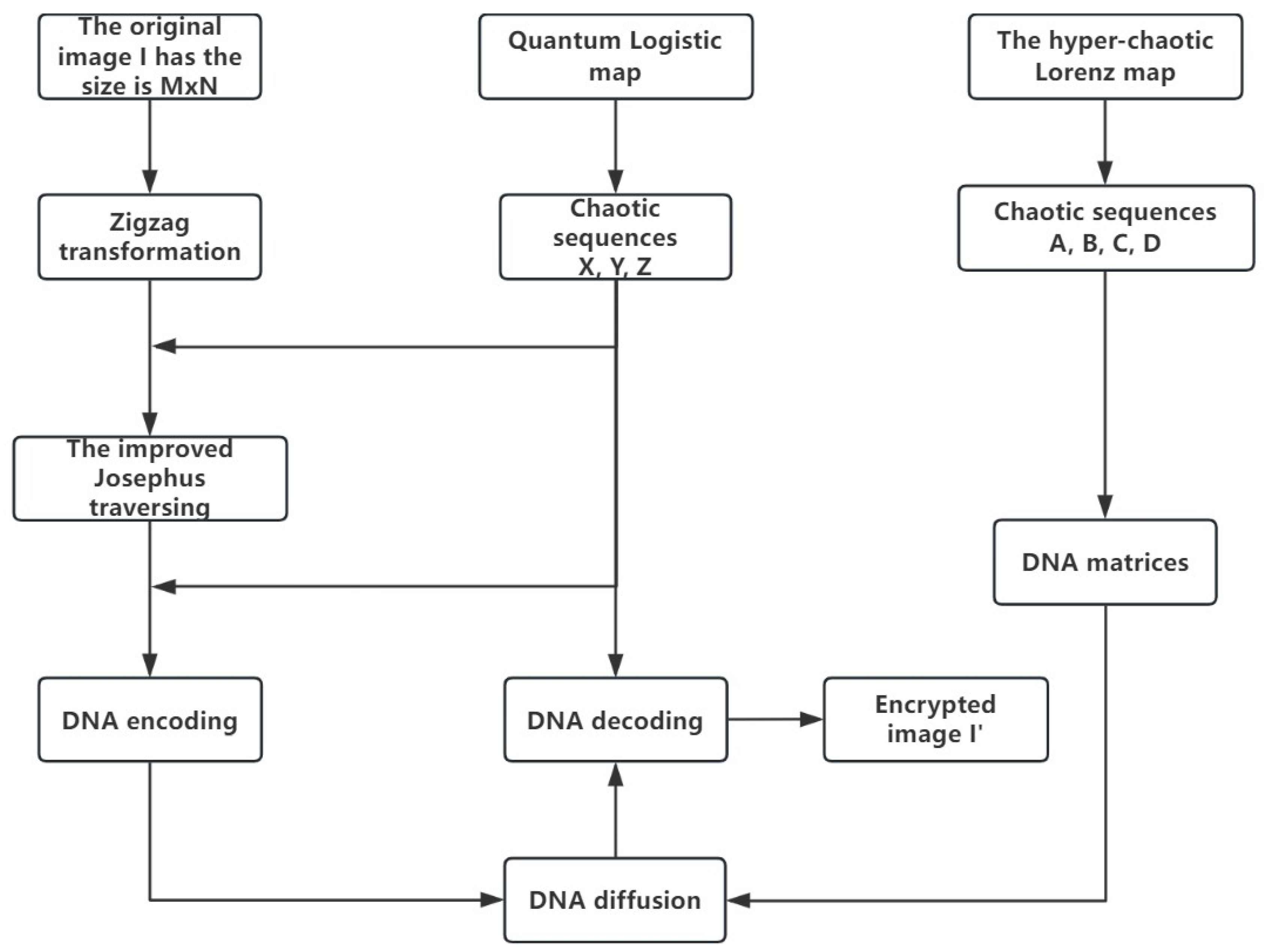
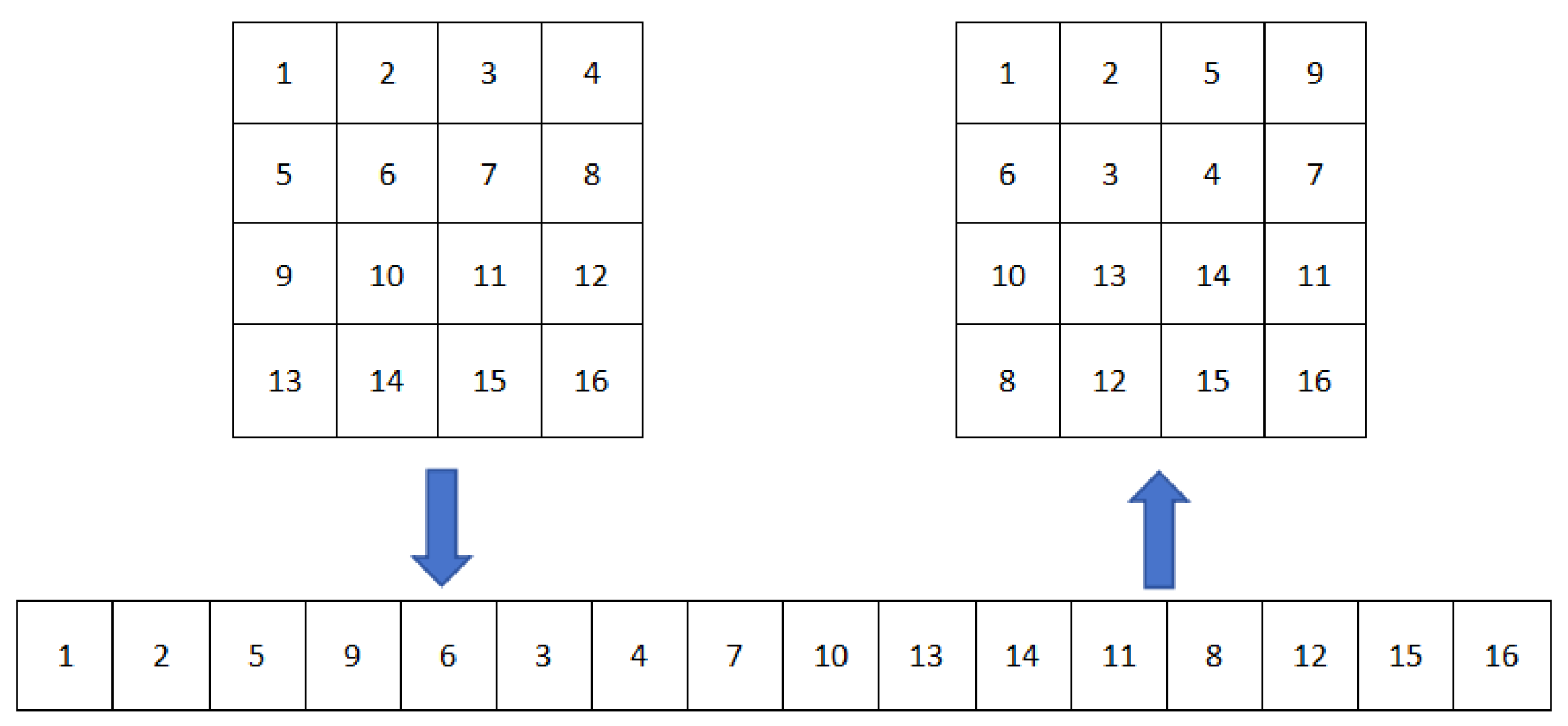
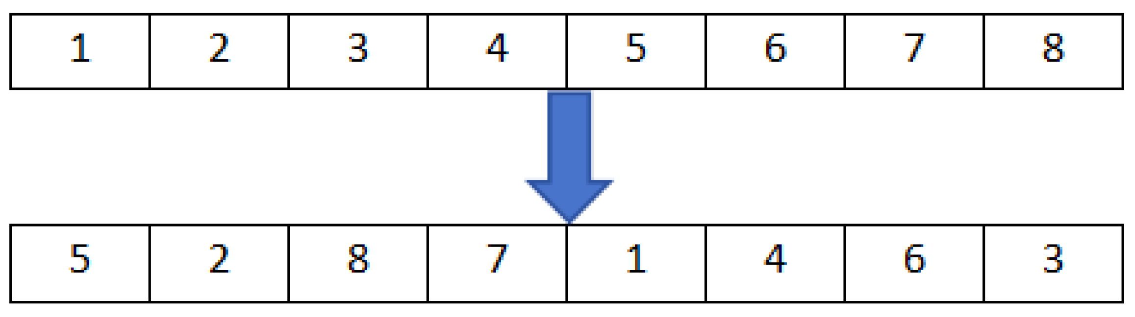
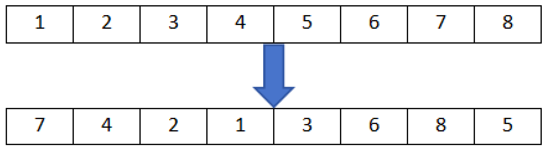
The following outlines the paper’s structure. In Section 2, we detail the chaotic maps adopted in the encryption scheme. Section 3 presents the DNA coding and operations. Section 4 discusses Zigzag transformation and Josephus traversing. Section 5 elaborates on the encryption theory and implementation stages of our proposed algorithm. In Section 6, we conducted experimental simulations and performed comprehensive security analyses on the algorithm. Furthermore, we contrast our findings with prior algorithms. Section 7 offers the conclusions and future prospects.

2. Chaotic Maps

2.1. Quantum Logistic Map

In 1990, Goggin and his team [36] put forward the Quantum Logistic map for the first time. In their research, they combined a kicked quantum system with an oscillator bath. Through this combination, they managed to obtain a Logistic map. What is special about this Logistic map is that it has quantum corrections of extremely low order. They found that as the dissipation parameter increases, so does the doubling route into classical behavior. The following is the expression for the quantum Logistic map [32]:

$$\{\begin{array}{ccc}{x}_{n+1}\hfill & =r\left(x_n-{\left|x_n\right|}^2\right)-r{y}_n,\hfill & \text{(1a)}\\ \hfill y_{n+1}& =-y_n{e}^{-2\beta }+e^{-\beta }r\left[(2-x_n-x_n^{*})y_n-x_n{z}_n^{*}-x_n^{*}{z}_n\right],\hfill & \text{(1b)}\\ \hfill z_{n+1}& =-z_n{e}^{-2\beta }+e^{-\beta }r\left[2(1-x_n^{*})z_n-2x_n{y}_n-x_n\right],\hfill & \text{(1c)}\end{array}$$

As defined in the equation, $x=\langle a\rangle$, $y=\langle \delta a^{†}\delta a\rangle$, $z=\langle \delta a\delta a\rangle$. In the map, $\beta$ serves as the dissipation parameter, with its value confined to the interval $\beta \in [6,+\infty )$. Meanwhile, r acts as the control parameter, having a range of $r\in [0,4]$. $x_n^{*}$ and $z_n^{*}$ are, respectively, the complex conjugates of x and z. Notably, when the initial values of x, y, and z are set to real numbers, then all the values coming out of the subsequent iterations will also be real numbers, i.e., $x_n^{*}=x$ and $z_n^{*}=z$. The initial values are restricted within the following ranges: $x\in (0,1)$, $y\in (0,0.1)$, and $z\in (0,0.2)$. It should be emphasized that the intermediate values of $\beta$, $y_n$, and $z_n\ne 0$ are considered here. Equation (1a) shares a similar structure with the Logistic map, incorporating additive noise. In fact, the noise here quantifies the magnitude of quantum corrections. As the number of iterations grows, and the quantum corrections $y_n$ and $z_n\to 0$ and the strong dissipation limit $\beta \to \infty$, the quantum Logistic map reduces to a classical Logistic map, which presents a period doubling route to chaos [37]. In particular, the randomness of the chaotic map is best when the parameter $r=3.99$ and $\beta \ge 6$, with a highly nonperiodic characteristic. Moreover, the interference and superposition introduced by quantum effects allow small changes to significantly affect the evolution of the system, resulting in complex and unpredictable behaviors and providing higher security and efficiency.

Figure 1 presents bifurcation diagrams for the quantum Logistic map. Compared to the classical Logistic map, this system significantly improves the chaotic characteristics by introducing quantum perturbation terms at the end of each iteration. The quantum perturbation mechanism brings three key advantages: Firstly, the system extends the effective chaotic range from the limited interval (3.57∼4.0) of the classical model to a wide region with $\beta >4$, enabling the chaotic behavior to remain stable over a broader parameter range. Secondly, the small perturbations introduced at each iteration not only eliminate the fixed points and stability windows observed in the classical system, but also completely avoid periodic behavior, while amplifying the butterfly effect and enhancing the sensitivity to initial conditions. Most importantly, the quantum perturbation causes the system’s state values to nearly uniformly fill the [0, 1] interval when $\beta >4$, significantly improving the randomness and uniformity of the sequence distribution. These improvements make the quantum Logistic map particularly suitable for high-security encryption scenarios, as it can generate higher-quality pseudorandom sequences.

2.2. The Hyper-Chaotic Lorenz Map

The hyper-chaotic Lorenz map builds upon the traditional Lorenz map structure, whose discovery was attributed to the American meteorologist Lorenz. In 1963, Lorenz [38] proposed the classical Lorenz map, consisting of three nonlinear ordinary differential equations. However, Lorenz later realized that if some modifications were made to the classical Lorenz map, a more complex and chaotic dynamical behavior could be achieved. Therefore, he added some nonlinear terms and extra driving forces to obtain the hyper-chaotic Lorenz map. As opposed to low-dimensional chaotic maps, the hyper-chaotic Lorenz map is characterized by high complexity, unpredictability, and a larger key space, making it capable of generating high-quality random number sequences. The expression for the hyper-chaotic Lorenz map [39] is given by

$$\left\{\begin{array}{c}\dot{x}=a\left(y-x\right)+w,\hfill \\ \dot{y}=cx-y-xz,\hfill \\ \dot{z}=xy-bz,\hfill \\ \dot{w}=-yz+rw.\hfill \end{array}\right.$$

(2)

In these equations, the rates of change, denoted as $\dot{x}$, $\dot{y}$, $\dot{z}$, and $\dot{w}$, correspond to the system state variables x, y, z, and w, respectively. The system parameters are a, b, c, and r. Under conditions where a is set to 10, b to 8/3, c to 28, and r falls within the range of −1.52 to −0.06, the Lorenz map exhibits a hyper-chaotic behavior. Consequently, using the Runge–Kutta method, one can generate four distinct random sequences from x, y, z, and w. After calculation, the four Lyapunov exponents [39] obtained at this time are as follows: ${\lambda }_1=0.3381$, ${\lambda }_2=0.1586$, ${\lambda }_3=0$, ${\lambda }_4=-15.1752$. As opposed to low-dimensional chaotic maps, one can find that the hyper-chaotic Lorenz map, with its four state variables and two positive Lyapunov exponents, exhibits a more intricate phase space structure and more complex trajectory characteristics, and it is capable of generating various types of chaotic behaviors, offering significant advantages in terms of both complexity and applicability. These features enable the hyper-chaotic Lorenz map to provide a larger and more complex key space. Such characteristics not only enhance the dimensionality of security but also make the dynamic behavior more complex and for a more unpredictable system.

3. DNA Coding and Operations

DNA coding refers to the composition of genes on a DNA molecule and how these genes are transcribed into RNA and translated into proteins. In 1994, Dr. Adleman from the University of California, USA, published a seminal paper in the journal Science exploring the possibilities of molecular biocomputational methods for DNA. He successfully solved a Hamiltonian path problem with seven vertices using biochemical methods, which demonstrated the feasibility of using DNA for specific computational purposes [26]. This study sparked interest in DNA-based molecular computing, and many of the advantageous properties of DNA, such as its high parallelism, vast storage capacity, high operational efficiency, and low energy consumption, were gradually recognized. In recent years, this field has garnered increasing attention from scholars, with DNA computing models and algorithms showing immense potential in fields such as bioinformatics, computer science, and biomedical research. Furthermore, DNA computing continues to attract the attention of both the academic and industrial communities worldwide. With advancements in technology and the development of theory, researchers have increasingly explored the combination of DNA computing and intelligent computational approaches like genetic algorithms, neural networks, fuzzy systems, and chaotic maps, providing new ideas and solutions for tackling complex problems [40,41,42].

3.1. DNA Coding

As the hereditary material in living cells, DNA adopts a double-helical structure, mainly situated in the nucleus and mitochondria. Its genetic units, genes, are composed of four deoxynucleotide bases: Adenine (A), Cytosine (C), Guanine (G), and Thymine (T). The double-helix structure of DNA is formed by two complementary strands coiled around each other, with hydrogen bonds between the base pairs linking them. The base pairing rule is that Adenine (A) bonds with thymine (T) via two hydrogen bonds, whereas guanine (G) links to cytosine (C) with three. These deoxynucleotides form the encoding sequence of DNA according to the nucleotide pairing principle.

The nucleotide pairing principle in DNA is conceptually similar to binary complement rules, such as 0 and 1, 00 and 11, 01 and 10 being complementary pairs. If we assign a 2-bit binary code to each base, four bases (A, T, C, G) can be encoded into four binary numbers (00, 01, 10, 11), resulting in 24 possible binary combinations. However, to comply with the base pairing principles of DNA sequences, only eight of these combinations are valid, as shown in

Table 1. Eight types of DNA encoding and decoding rules.

Rules	1	2	3	4	5	6	7	8
11	A	A	T	T	G	G	C	C
00	T	T	A	A	C	C	G	G
10	C	G	C	G	T	A	T	A
01	G	C	G	C	A	T	A	T

.

To further extend the pairing principles of DNA sequences, we now explore how these principles are applied to image encoding. In this study, 8-bit grayscale images are employed, where the pixel intensity values fall within the interval [0, 255]. Here, 0 symbolizes the darkest shade, 255 represents the brightest white, and the intermediate values represent various degrees of gray. In this manner, a decimal pixel value can be converted into an 8-bit binary code indicating its grayscale level. For instance, the pixel value of 210 has a binary representation of “11010010”. According to encoding Rule 1 listed in Table 1, its corresponding DNA sequence is “AGTC". Alternatively, if Rule 8 is used for encoding, the DNA sequence obtained would be “CTGA”. This demonstrates that the DNA sequence obtained depends on the chosen encoding rule. Similarly, in the decoding process, only the correct encoding rule can successfully decode the sequence. If mismatches between encoding and decoding rules occur, this will lead to failure in obtaining the accurate pixel value. For example, decoding the DNA sequence “AGTC” generated by Rule 1 using Rule 1 will yield the original binary sequence “11101010”. However, if a different encoding rule, such as Rule 8, is applied to interpret the identical DNA strand “AGTC”, the resulting binary sequence “10000111” will differ from the original binary sequence “11010010”. Therefore, maintaining consistency between encoding and decoding rules is a prerequisite for accurate reconstruction of the original image.

3.2. DNA Operations

As DNA computing progresses, scholars have put forward DNA-based arithmetic operations including addition, subtraction, and XOR. However, unlike traditional binary arithmetic, each DNA encoding rule corresponds to a specific DNA operation result. That is, the eight different DNA encoding rules are associated with eight different sets of DNA addition and subtraction rules. In this study, Rule 1 from Table 1 is selected for the operations, and the DNA addition, subtraction, and XOR rules are separately illustrated in

Table 2. DNA sequence addition result according to Rule 1.

+	A-11	T-00	C-10	G-01
A-11	C-10	A-11	G-01	T-00
T-00	A-11	T-00	C-10	G-01
C-10	G-01	C-10	T-00	A-11
G-01	T-00	G-01	A-11	C-01

,

Table 3. DNA sequence subtraction result according to Rule 1.

-	A-11	T-00	C-10	G-01
A-11	T-00	A-11	G-01	C-10
T-00	G-01	T-00	C-10	A-11
C-10	A-11	C-10	T-00	G-01
G-01	C-10	G-01	A-11	T-00

and

Table 4. DNA sequence XOR result according to Rule 1.

XOR	A-11	T-00	C-10	G-01
A-11	T-00	A-11	G-01	C-10
T-00	A-11	T-00	C-10	G-01
C-10	G-01	C-10	T-00	A-11
G-01	C-10	G-01	A-11	T-00

.

As seen in Table 2, Table 3 and Table 4, once the DNA encoding rule has been determined, its corresponding operation results are also fixed. Moreover, the addition and subtraction results for a given DNA encoding rule are uniquely determined. In our encryption work, we employ DNA dynamic technology for DNA encoding, addition, and XOR operations, to achieve pixel diffusion in images, thus improving the algorithm’s level of complication and protection.

4. Zigzag Transformation and Josephus Traversing

4.1. Zigzag Transformation

Zigzag transformation [43] is a method for rearranging the pixels of a two-dimensional image following a zigzag path. Starting from the top-left corner, the entire matrix is traversed in a “Z”-shaped pattern to achieve a scrambling effect. The specific implementation is as follows: Consider a $4\times 4$ matrix, with the top-left element as the starting point. The elements are sequentially extracted by scanning in a “Z”-shaped pattern, and the elements obtained through scanning are placed in a one-dimensional array. This array is then rearranged into a $4\times 4$ matrix by grouping the elements in sets of four. The specific procedure is illustrated in Figure 2.

4.2. Josephus Traversing

In the disciplines of computer science and mathematics, the Josephus problem [44] stands as a classic example. In algorithmic programming, this type of problem is also referred to as the Josephus circle or the “handkerchief problem”. Josephus traversing is a scrambling method derived from the classic Josephus problem. In the traditional Josephus problem, a group of N individuals are positioned in a circle. Beginning with the first person, they count up to M, and the M-th person is eliminated. Counting resumes from the next person after the one who was eliminated, and the process repeats until only one person remains. By recording the sequence in which people are eliminated, a new arrangement is obtained, which is known as Josephus scrambling. The Josephus problem is represented by the function $f(N,M)$, where N denotes the total number of elements, and M represents the Josephus distance, which indicates the elimination of the M-th element. For example, for the sequence $\{1,2,3,4,5,6,7,8\}$, applying the function $f(8,5)$ will result in a new sequence $\{5,2,8,7,1,4,6,3\}$, as shown in Figure 3.

To introduce more variability into the Josephus traversing algorithm, a perturbation can be added by introducing an elimination starting point, denoted as S [45]. The improved Joseph traversing can then be described as follows: N people are arranged in a circle, and the counting begins from the S-th person, and every time the count reaches M, the M-th person is eliminated. Counting resumes from the person immediately following the eliminated one, and the process repeats until only one person remains. By recording the sequence of eliminated individuals, a new arrangement is obtained, which is known as the modified Josephus traversing. The improved Josephus traversing is expressed as the function $f(N,S,M)$, with N being the total quantity of elements, S serving as the point from which elimination commences, and M is the Josephus distance, which determines the elimination of the M-th element. For example, for the sequence $\{1,2,3,4,5,6,7,8\}$, applying the function f(8, 3, 5) will result in the new sequence $\{7,4,2,1,3,6,8,5\}$, as shown in Figure 4. Clearly, $f(N,S,M)$ introduces greater variability in the scrambled sequence compared to $f(N,M)$.

5. Algorithm Design

5.1. Encryption Theory

The following describes the algorithm design strategy adopted in this paper:

(1)

The first scrambling operation is performed using the Zigzag transformation algorithm, followed by a second scrambling operation that combines the improved Josephus traversal with a quantum Logistic map.

(2)

The quantum Logistic map is then used to dynamically select DNA encoding, which transforms the scrambled image into a DNA matrix.

(3)

The pixel diffusion operation is carried out by dynamically selecting DNA addition and XOR rules using the quantum Logistic map and a hyper-chaotic Lorenz map, respectively.

(4)

Finally, the hyper-chaotic Lorenz map is employed to make a dynamic choice of the DNA decoding rules.

Quantum Logistic map is a technique capable of generating highly random sequences, which makes cryptanalysis more challenging and improves the robustness of encryption methods. The main operation is as follows. First, using Equation (1), three pseudorandom sequences of lengths N, N, and $4\times M\times N$ are generated:

$$\left\{\begin{array}{cc}\hfill X& =\{x_1,x_2,x_3,\dots ,x_N\},\hfill \\ \hfill Y& =\{y_1,y_2,y_3,\dots ,y_N\},\hfill \\ \hfill Z& =\{z_1,z_2,z_3,\dots ,z_{4\times M\times N}\}.\hfill \end{array}\right.$$

In this case, M stands for the row count of the original image pixels, and N stands for the column count. Then, the following operations are performed on the random sequences X, Y, and Z:

$$\left\{\begin{array}{c}{x}_i=mod\left(floor(abs\left(x_i\right)\times {10}^8),N\right)+1,i=1,2,\dots ,N,\hfill \\ y_i=mod\left(floor(abs\left(y_i\right)\times {10}^8),N\right)+1,i=1,2,\dots ,N,\hfill \\ z_i=mod\left(floor(abs\left(z_i\right)\times {10}^8),8\right)+1,i=1,2,\dots ,4\times M\times N.\hfill \end{array}\right.$$

(3)

Here, $floor\left(x\right)$ denotes the greatest integer that does not surpass x, $abs\left(x\right)$ represents the absolute value quantity of x, and $mod(a,b)$ denotes the remainder when a is divided by b. After computation, the numbers in the random sequences X and Y are modified to random integers falling within the scope of $[1,N]$, while the numbers of random sequence Z are modified to random integers falling within the scope of $[1,8]$.

The second scrambling operation is performed on the image using the improved X and Y random sequences and the improved Josephus traversing. The Josephus step formula for the i-th row is as follows:

$$f(N,S_i,Q_i)=f(N,x_i,y_i),i=1,2,3,\dots ,M.$$

(4)

For instance, with an image resolution of $256\times 256$ and $i=25$, where $x_{25}=96$ and $y_{25}=157$, the function $f(N,Si,Qi)=f(256,96,157)$, which means that the 256 elements in the 25th row of the image matrix are subjected to the Josephus traversing operation, starting from the 96th element, with a Josephus distance of 157.

And the improved random sequence $Z=\{z_1,z_{2,}{z}_3,\dots ,z_{4\times M\times N}\}$ is then employed to dynamically select the DNA encoding and addition rules in the subsequent steps.

The hyper-chaotic Lorenz map, with its unique hyper-chaotic state, enhances the sensitivity and randomness of system, ensuring that the generated key sequences exhibit high unpredictability and are difficult to replicate. The key operations are outlined below: using Equation (2), four pseudo-random sequences of lengths $8\times M\times N$, $4\times M\times N$, $8\times M\times N$ and $4\times M\times N$ are generated, denoted as follows:

$$\left\{\begin{array}{c}A=\{a_1,a_2,a_3,\dots ,a_{8\times M\times N}\},\hfill \\ B=\{b_1,b_2,b_3,\dots ,b_{4\times M\times N}\},\hfill \\ C=\{c_1,c_2,c_3,\dots ,c_{8\times M\times N}\},\hfill \\ D=\{d_1,d_2,d_3,\dots ,d_{4\times M\times N}\}.\hfill \end{array}\right.$$

The next steps involve performing operations on the random sequences A, B, C, and D:

$$\left\{\begin{array}{c}{a}_i=mod\left\{floor\left\{[abs\left(a_i\right)-floor\left(abs\left(a_i\right)\right)]\times {10}^{16}\right\},2\right\},\hfill \\ b_i=mod\left\{floor\left\{[abs\left(b_i\right)-floor\left(abs\left(b_i\right)\right)]\times {10}^{16}\right\},8\right\}+1,\hfill \\ c_i=mod\left\{floor\left\{[abs\left(c_i\right)-floor\left(abs\left(c_i\right)\right)]\times {10}^{16}\right\},2\right\},\hfill \\ d_i=mod\left\{floor\left\{[abs\left(d_i\right)-floor\left(abs\left(d_i\right)\right)]\times {10}^{16}\right\},8\right\}+1.\hfill \end{array}\right.$$

(5)

where the numbers $a_i\left(c_i\right)$ in the random sequences $A\left(C\right)$ are converted into random binary values 0 or 1, serving as the foundation for constructing the DNA matrix. Simultaneously, the values $b_i\left(d_i\right)$ in the random sequences $B\left(D\right)$ are converted into arbitrary integers within [1, 8], guiding the application of the DNA encoding rules.

5.2. Encryption Steps

Assume the original grayscale image I has a size of $M\times N$. The encryption process is depicted in Figure 5, and can be described as follows:

Step 1 The original grayscale image I undergoes a conversion process to form a two-dimensional matrix $I_1$ with the dimensions $M\times N$.

Step 2 The matrix $I_1$ is subjected to Zigzag transformation, resulting in the first scrambling matrix $I_2$.

Step 3 Employing the quantum Logistic map (see Equation (1)), four pseudorandom sequences are generated and denoted as X, Y, and Z, with respective lengths of N, N, and $4\times M\times N$. Additionally, four pseudorandom sequences, A, B, C, and D, are generated through the hyper-chaotic Lorenz map (see Equation (2)), with lengths $8\times M\times N$, $4\times M\times N$, $8\times M\times N$ and $4\times M\times N$, respectively.

Step 4 The sequences X, Y, and Z undergo arithmetic transformations (see Equation (3)), while sequences A, B, C, and D are processed with arithmetic operations specified (see Equation (5)).

Step 5 The improved Josephus traversing is applied to each row of the matrix $I_2$, where the step size for the i-th row is determined by Equation (4). This results in the matrix $I_3$, thus completing the two scrambling processes.

Step 6 Subsequently, the scrambled matrix $I_3$ is transformed into a binary matrix $I_4$.

Step 7 Guided by the values of the sequence Z, the DNA encoding rules specified in Table 1 are dynamically chosen. Afterwards, DNA encoding is performed on each two-bit binary number within the binary matrix $I_4$, resulting in the generation of the DNA matrix $I_5$.

Step 8 Based on the values of sequences B and D, the DNA encoding rules are selected from Table 1, and the binary bits in sequences A and C are encoded into DNA, generating DNA matrices $I_6$ and $I_7$, respectively.

Step 9 A DNA addition operation is performed on matrices $I_6$ and $I_7$ guided by the values in sequence Z, by dynamically selecting the addition rule aligned with the eight DNA codification principles listed in Table 1, yielding the DNA matrix $I_8$.

Step 10 Using the DNA encoding rules from Table 1, one of which is dynamically selected based on the values in sequence B, matrices $I_5$ and $I_8$ perform the corresponding XOR operation, leading to the formation of the DNA matrix $I_9$.

Step 11 The DNA matrix $I_9$ is decoded back into a binary matrix $I_{10}$ using the appropriate DNA decoding rule selected from Table 1, in accordance with the values of sequence D.

Step 12 Finally, through the conversion of the binary matrix $I_{10}$ to a decimal matrix, the encrypted image $I^{\prime }$ is obtained.

The entire image encryption algorithm comprises encryption and decryption algorithms. Given that the suggested cryptographic system is a symmetric encryption model, the decryption process is essentially the reverse of the encryption process. As such, the details of the decryption process will not be elaborated upon herein.

6. Experimental Simulation and Safety Analysis

6.1. Experimental Simulation

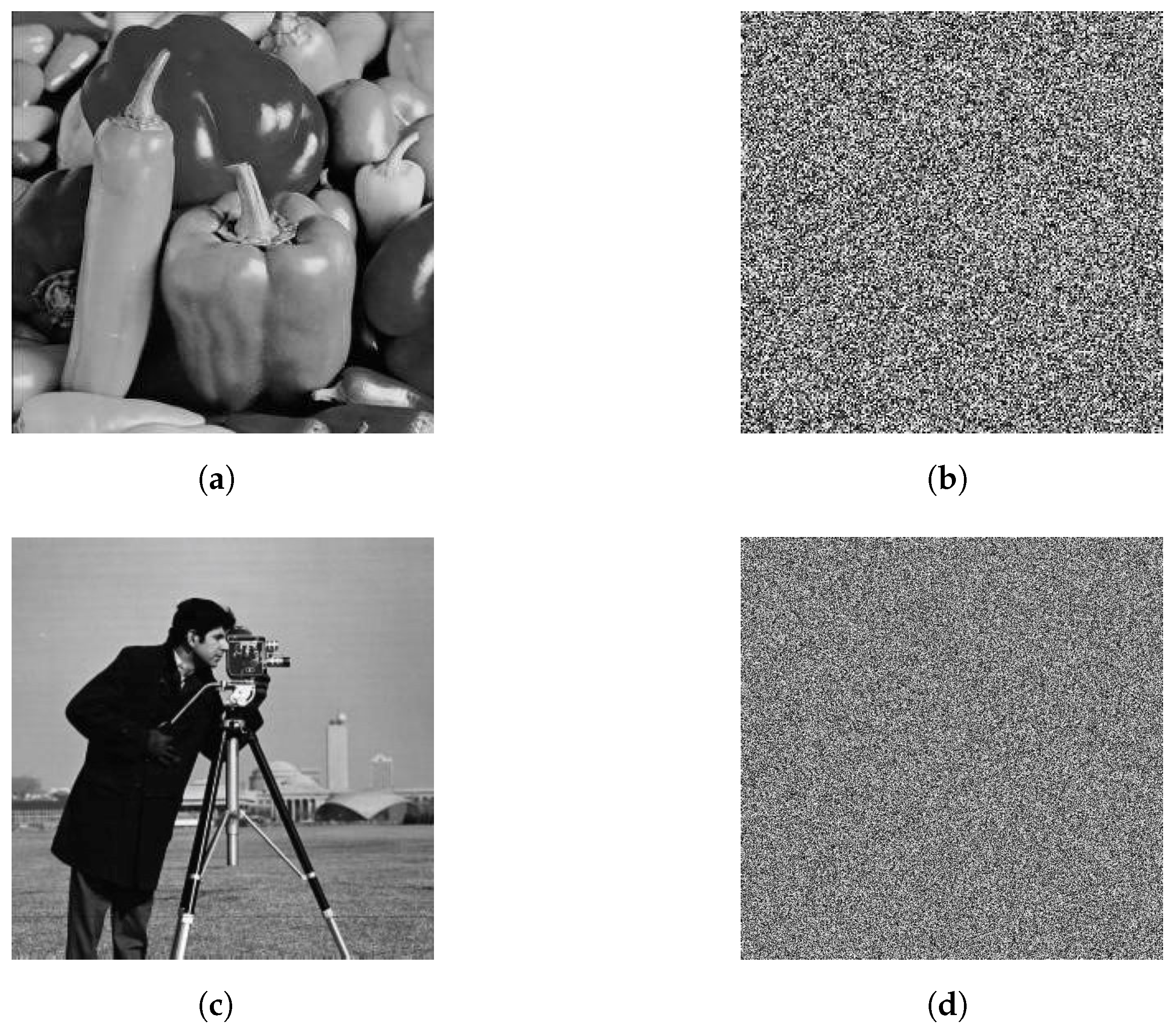
The proposed algorithm was simulated in a Python 3.13.3 (64-bit) environment. When conducting the experiments, $256\times 256$ (Peppers) and $512\times 512$ (Cameraman) grayscale images were selected as the original images. The initial values for the quantum Logistic map were $x_1=0.4347$, $y_1=0.0563$ and $z_1=0.1384$, with parameters $\beta =6$ and $r=3.99$. The initial parameter values for the hyper-chaotic Lorenz map were $x_0=0.8162$, $y_0=0.0656$, $z_0=0.3876$, and $w_0=0.9680$. Figure 6 displays the original and encrypted images. Clearly, the encrypted image bears no visual resemblance to the original and provides no insight into its content. Therefore, the algorithm effectively encrypted the image and ensured robust safeguarding of its original data.

Image source: Figure 6a was obtained from https://ccia.ugr.es/cvg/dbimagenes/, accessed on 8 October 2024; Figure 6c was sourced from the MIT link https://dome.mit.edu/handle/1721.3/195767, accessed on 8 October 2024.

6.2. Key Space Analysis

To safeguard digital images effectively, a robust encryption method must feature an extensive key space capable of withstanding brute-force attempts. As a rule of thumb, the encryption key’s complexity should meet or exceed a $2^{100}$ threshold to provide adequate protection. In our encryption algorithm, the quantum Logistic map and the hyper-chaotic Lorenz map serve as the core components for image encryption. The entire encryption operation relies on the following keys:

(1)

Parameters of the quantum Logistic map: $\beta$, r, and initial values $x_1$, $y_1$, $z_1$.

(2)

Initial values of the hyper-chaotic Lorenz map: $x_0$, $y_0$, $z_0$, and $w_0$.

where the parameters and initial values ranges for the quantum Logistic map are as follows: $\beta \in [6,+\infty )$, $r\in [0,4]$ and $x\in (0,1)$, $y\in (0,0.1)$, $z\in (0,0.2)$. Given that a quantum Logistic map demonstrates an extraordinary sensitivity to parameters and initial values (with a sensitivity of ${10}^{-16}$) [33], the key space for the quantum Logistic map can be ascertained using the subsequent approach: the parameter key space $S_{\beta }=S_r=4\times {10}^{16}$, the initial value key spaces $S_x={10}^{16}$, $S_y=S_z={10}^{15}$. Therefore, the total key space for the quantum Logistic map is $S_1=S_{\beta }\times S_r\times S_x\times S_y\times S_z=1.6\times {10}^{79}\approx 2^{263}$. Similarly, since the precision of the initial values in the hyper-chaotic Lorenz map is ${10}^{-14}$, the key space for the hyper-chaotic Lorenz map is $S_2={10}^{14\times 4}={10}^{56}\approx 2^{187}$.

Following the preceding examination, the encryption algorithm’s total key space is $S=S_1\times S_2=2^{450}\gg 2^{100}$. The enormous size of this key space provides robust protection against brute-force cracking attempts, validating the encryption method’s exceptional security credentials and its reliable defense against such adversarial intrusion strategies.

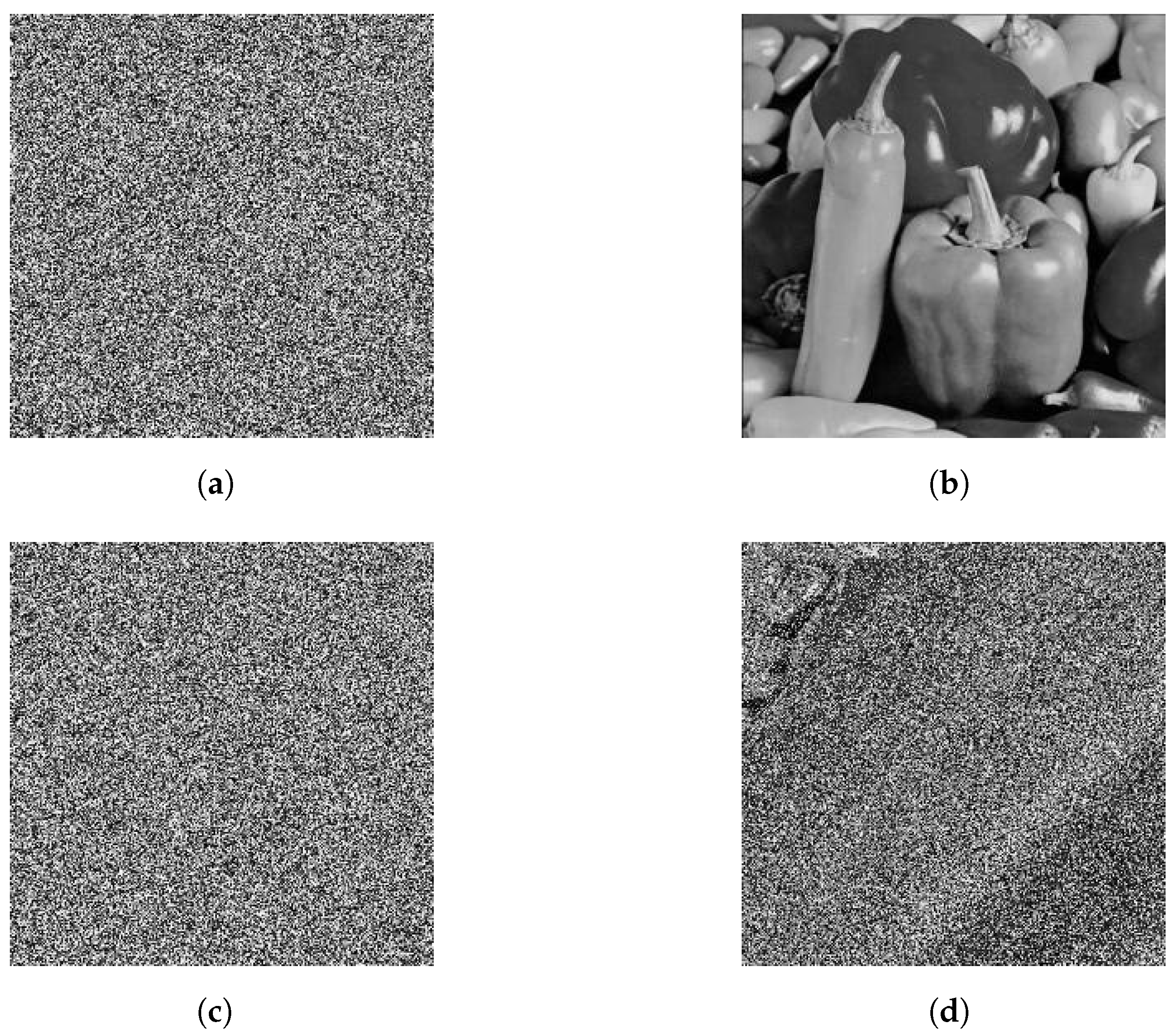
6.3. Key Sensitivity Analysis

A well-performing image encryption method hinges on a key that is sensitive—tiny alterations in the key must generate a unique decrypted image, ensuring security. In this particular approach, the key encompasses parameters and initial conditions for both the quantum Logistic map and the hyper-chaotic Lorenz map. To assess how responsive the quantum Logistic map is to perturbations to its initial state, we carried out a detailed examination, using the iconic $256\times 256$ Peppers image as a benchmark to verify its sensitivity. Under the initial parameters of $x_1=0.4347$, $y_1=0.0563$ and $z_1=0.1384$, the system-produced encrypted image is depicted in Figure 7a, and when decrypted with the same parameters, the original image was perfectly restored, as in Figure 7b. During the experiment, it was found that when a minute perturbation of ${10}^{-16}$ or ${10}^{-15}$ was applied to the initial values ($x_1=0.4347+{10}^{-16}$, $y_1=0.0563+{10}^{-15}$ and $z_1=0.1384+{10}^{-15}$), the system exhibited significant sensitivity. Firstly, the encrypted result in Figure 7c exhibits visually distinguishable differences compared to the standard encrypted image Figure 7a. Secondly, although the deviation in the key was minimal, decryption using the perturbed parameters failed to fully restore the original image, see Figure 7d. This phenomenon reveals the unique dynamical characteristics of the quantum Logistic map: the system exhibits a high degree of sensitivity to initial conditions, where even minute differences in parameters are exponentially amplified through iterative operations, ultimately leading to a complete alteration of the output sequence. The experimental results indicate that the quantum Logistic map demonstrated superior performance in terms of parameter sensitivity, thereby providing a theoretical basis for the development of high-security image encryption systems.

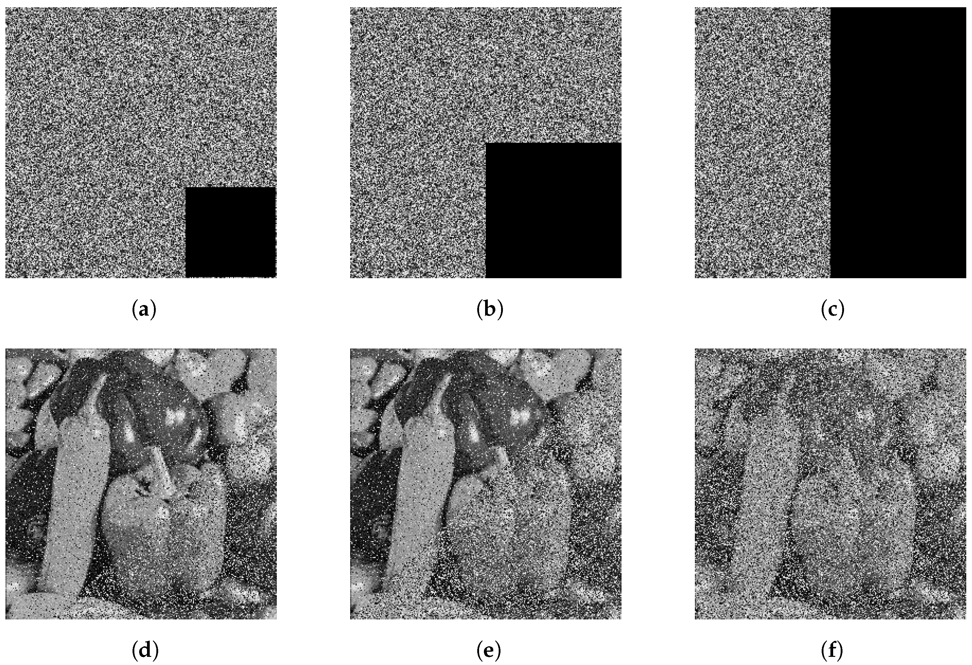
6.4. Crop Attack Analysis

The rise of digital imagery in vital sectors like cyber security, healthcare, and military messaging has highlighted the necessity for robust image encryption algorithms for resilience against interference. In real-world scenarios, encrypted images face numerous attack tactics, with crop attacks being a prevalent risk. To systematically assess the algorithm’s resilience to these attacks, this study designed a tiered testing scheme. We simulated crop attack scenarios by artificially setting three progressive levels of data corruption: mild ($11\%$ data removal), moderate ($25\%$ removal), and severe ($50\%$ removal), as illustrated in Figure 8. The visual information shows encrypted images subjected to progressive cropping (Figure 8a–c) alongside their reconstructed counterparts (Figure 8d–f). Remarkably, even when half the encrypted data were deliberately discarded (Figure 8f), the decryption process successfully preserved the fundamental structure and key visual elements of the source image. This phenomenon not only fully demonstrates the remarkable robustness of the proposed algorithm, but also provides crucial support for the practical application of the algorithm in unreliable channels.

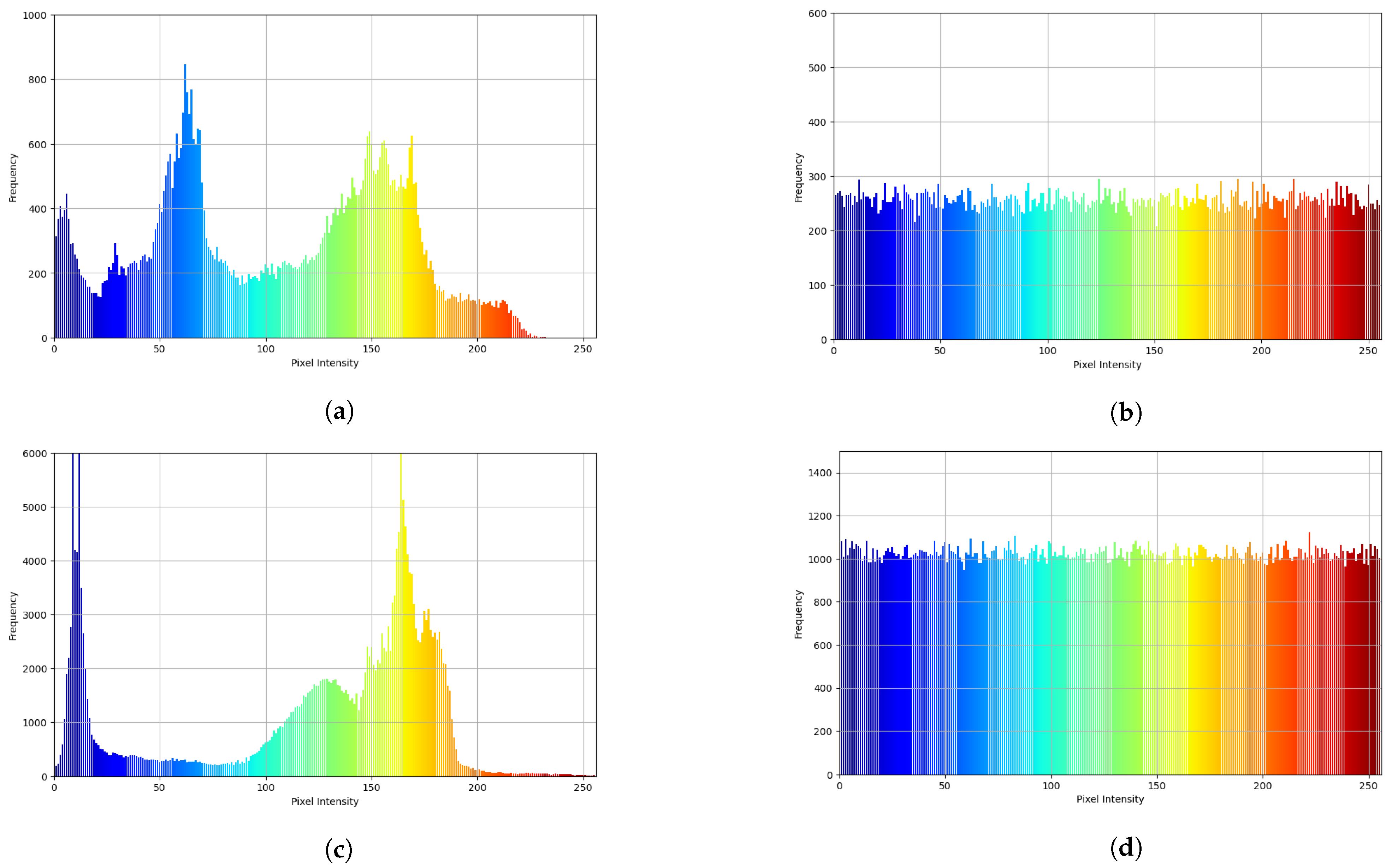
6.5. Histogram Analysis

An image histogram essentially captures the statistical spread of pixel values across an image. Generally manifested as a graphical plot with 256 discrete bins, where each bin corresponds to a unique grayscale value within the range of 0–255, and the magnitude of each bin’s height precisely measures the prevalence of that grayscale level in the image. By carefully analyzing the histogram, one gains a clear understanding of how grayscale values are distributed throughout the image. In the context of encryption algorithms, a high-quality algorithm should yield an encrypted image with a pixel value distribution that is as evenly dispersed as possible, as this directly correlates with enhanced encryption performance. In the present study, we conducted a detailed examination and comprehensive comparison of the histograms for both the original and encrypted versions of the Peppers and Cameraman images, as depicted in Figure 9.

The analysis showed that the grayscale distributions of the original Peppers and Cameraman images exhibited multiple peaks and valleys, showing distinct statistical characteristics. Conversely, the corresponding encrypted images had a grayscale distribution that was more concentrated, without obvious patterns or regularities, and lacking clear statistical features. This outcome demonstrated that the encryption operation had reliably scrambled and concealed the original image data. Thus, the suggested algorithm can robustly withstand statistical assault and exhibits strong security features.

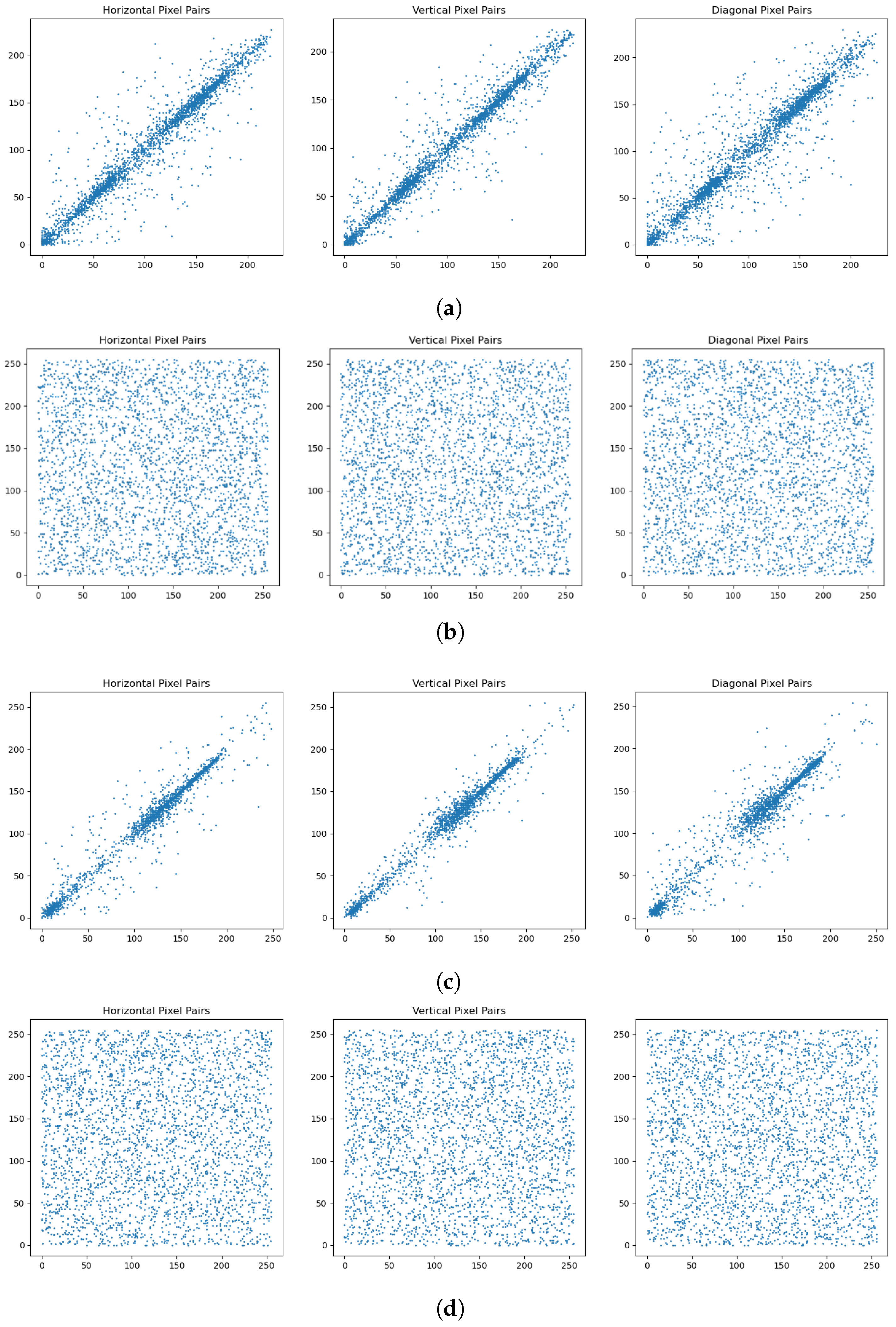
6.6. Adjacent Pixel Correlation Analysis

In image processing and computer vision, analyzing the correlation between neighboring pixels is a fundamental technique for evaluating the alignment of grayscale or color values. This relationship is quantified using the correlation coefficient r, a statistical metric that measures the intensity and direction of the linear association between two variables. The value of r ranges from $-1$ to 1: 1 denotes a perfect positive correlation, where an increase in one variable is accompanied by a proportional increase in the other; $-1$ indicates a perfect negative correlation, where one variable decreases proportionally as the other increases; and 0 signifies no linear relationship between the variables. The strength of the correlation is reflected in the magnitude of $\left|r\right|$, where higher absolute values indicate stronger associations. Conventionally, variables are considered highly correlated when $\left|r\right|$ falls within the interval [0.7, 1].

In our work, we arbitrarily picked 3000 corresponding pixel pairs from both the original and the ciphered images, and constructed two sequences $X=\{X_1,X_2,X_3,\dots ,X_{3000}\}$ and $Y=\{Y_1,Y_{2,}{Y}_3,\dots ,Y_{3000}\}$ based on their corresponding grayscale values [46]. The mathematical expressions for determining the covariance and variance values are given as follows:

$$\left\{\begin{array}{c}cov(X,Y)={\displaystyle \frac{1}{N}}\sum _{i=1}^N\left(X_i-E\left(X\right)\right)\left(Y_i-E\left(Y\right)\right),\hfill \\ D\left(X\right)={\displaystyle \frac{1}{N}}\sum _{i=1}^N{\left(X_i-{\displaystyle \frac{1}{N}}\sum _{i=1}^N{X}_i\right)}^2,\hfill \\ D\left(Y\right)={\displaystyle \frac{1}{N}}\sum _{i=1}^N{\left(Y_i-{\displaystyle \frac{1}{N}}\sum _{i=1}^N{Y}_i\right)}^2.\hfill \end{array}\right.$$

(6)

The coefficient of association between neighboring pixels [33] can be determined by applying the formula below:

$$r={\displaystyle \frac{cov(X,Y)}{\sqrt{D\left(X\right)}\sqrt{D\left(Y\right)}}}.$$

(7)

Following this, we analyzed the pixel correlation for 3000 random adjacent pairs in the original and encrypted images across the horizontal, vertical, and diagonal axes. To thoroughly examine these correlations, Figure 10 illustrates the correlation patterns between neighboring pixels along three axes for both the Peppers and Cameraman images, comparing their original and encrypted states. Additionally,

Table 5. Correlation coefficient comparison of encrypted images in three directions.

Correlation	Horizontal	Vertical	Diagonal
Peppers (our)	−0.0014	−0.0004	−0.0081
Cameraman (our)	0.0028	−0.0064	−0.0036
Ref. [33] of Peepers	0.0066	−0.0026	0.0041
Ref. [44] of Peepers	0.0021	0.0084	0.0007
Ref. [45] of Cameraman	0.0082	0.0019	0.0088

provides a quantitative comparison of these encrypted image correlations against the results documented in Refs. [33,44,45].

Figure 10 illustrates the significant difference in pixel correlation between the original and encrypted images. The original image exhibits a positive correlation among pixel grayscale values in the horizontal, vertical, and diagonal orientations, with pronounced correlations. On the contrary, the encrypted image shows nearly zero correlation between adjacent pixels in these three directions, indicating that the original image’s pixel coherence has been disrupted. The encrypted image, therefore, exhibits no significant correlation in any direction. An examination of the correlation metrics presented in Table 5 indicates that for the Peppers image, our encryption algorithm yielded lower correlation values in both the horizontal and vertical directions. Similarly, for the Cameraman image, our encryption approach reduced the horizontal and diagonal correlation. These findings confirm that the proposed algorithm effectively mitigated correlation analysis, impeding attackers from extracting meaningful information from adjacent pixels and thereby bolstering the security and efficacy of the image encryption.

6.7. Information Entropy Analysis

Information entropy quantifies information uncertainty. In information theory, it measures a random variable’s unpredictability. Higher entropy values denote greater uncertainty and more information. Conversely, lower entropy indicates less uncertainty and a lower information content. An ideal and completely random image has an information entropy of 8. Therefore, an image whose entropy value approaches the ideal 8 has more randomly distributed pixel values, thereby offering greater protection against attacks. The information entropy formula for images [47] is defined as

$$H\left(X\right)=-\sum _{i=0}^{L-1}p\left(X_i\right)lo{g}_{2}p\left(X_i\right).$$

(8)

In our analysis, as depicted in

Table 6. Information entropies of the original and encrypted images.

Entropy	The Original Image	The Encrypted Image
Peppers (our)	7.5803	7.9974
Cameraman (our)	7.0624	7.9994
Ref. [33] of Peepers	-	7.9973
Ref. [45] of Peepers	7.5819	7.9968
Ref. [33] of Cameraman	-	7.9973

, we present the information entropy metrics for images that were encrypted using the methodologies outlined in Refs. [33,45] and our newly proposed technique. The total number of grayscale levels, denoted as L, was fixed at 256 for this investigation.

As tabulated in Table 6, the entropy metrics for images secured by the methods detailed in Refs. [33,45] and our suggested algorithm are presented.

Evidently, compared with the original, the encrypted version demonstrated entropy levels that aligned more closely with the ideal theoretical value, indicating a near-random distribution, with minimal discernible patterns. Our findings reveal that the encryption method employed here achieved a superior entropy performance relative to the techniques referenced in Refs. [33,45], as it more accurately approximated the expected disorder characteristics of a securely encrypted image. Specifically, the method exhibited a more uniform pixel distribution, making it significantly more resistant to entropy-based attacks.

6.8. Differential Attack Analysis

A differential attack is a cryptanalytic method designed to assess the robustness of encryption systems. This approach examines how minor modifications to input data, such as altering a single pixel, can produce measurable variations in the encrypted output. By analyzing these discrepancies, cryptographers can evaluate the vulnerability of cryptographic algorithms to such targeted manipulations. Specifically, a differential attack measures how much the encrypted data changes when the encryption key is slightly modified. In our work, we used NPCR and UACI to measure the resilience of the algorithm against differential attacks.

NPCR (Number of Pixels Change Rate) measures encrypted image sensitivity and encryption process efficacy relative to the original images. It measures the proportion of differing pixel values at matching locations across two images (typically the original and encrypted image, or two encrypted images using different keys). An NPCR value close to the ideal $99.6094\%$ indicates high key sensitivity and strong differential-attack resistance, thereby indicating a higher-security encryption algorithm. The NPCR [45] computation formula is given below:

$$NPCR={\displaystyle \frac{1}{M\times N}}\sum _{i=1}^M\sum _{j=1}^{N}D(i,j)\times 100\%.$$

(9)

UACI (Unified Average Changing Intensity) is utilized to gauge the dissimilarity between the encrypted and original images and assess the encryption’s effectiveness. It primarily measures the average change intensity of pixel values, reflecting the extent of detail variation between the encrypted image and the original one. The ideal UACI value is $33.4635\%$, and the nearer an obtained value is to this standard, the greater the key sensitivity and the better the resistance against differential attacks, signifying a more secure encryption method. The following equation outlines the UACI calculation method [45]:

$$UACI={\displaystyle \frac{1}{M\times N}}\sum _{i=1}^M\sum _{j=1}^N{\displaystyle \frac{\left|c_1(i,j)-c_2(i,j)\right|}{255}}\times 100\%.$$

(10)

According to the established formula, M represents the total rows, while N corresponds to the columns in the image. The pixel intensities at coordinates $(i,j)$ are designated as $C_1(i,j)$ for the original image and $C_2(i,j)$ for its encrypted counterpart. The difference metric $D(i,j)$ is 0 when $C_1(i,j)$ and $C_2(i,j)$ share identical values; conversely, it assumes a value of 1 whenever a discrepancy exists between them.

In our research, we performed a differential attack analysis on the chosen Peppers and Cameraman images.

Table 7. NPCR and UACI values of the encryption images.

Figure	NPCR	UACI
Peppers	$99.6078\%$	$30.9265\%$
Cameraman	$99.6154\%$	$31.1348\%$
Ref. [33] of Peepers	$99.60\%$	$29.60\%$
Ref. [45] of Peepers	$99.5803\%$	$33.4324\%$
Ref. [33] of Cameraman	$99.60\%$	$31.13\%$

presents the NPCR and UACI metrics for the encrypted images, together with the relevant results from Refs. [33,45]. Evidently, the NPCR values obtained by our encryption method are closer to 8, indicating that the algorithm exhibited excellent encryption performance and practical applicability.

6.9. Key Stream Correlation Analysis

When assessing encryption security, we should focus on the independence of chaotic sequences from plaintext to resist chosen plaintext attacks, for which the Pearson correlation coefficient and p-value serve as critical analytical indicators. The Pearson correlation coefficient assesses the intensity and direction of the linear association between any two variables, with its detailed definition and formula provided in Section 6.6 (Equation (7)). The p-value is an indicator used for testing the significance of the correlation. The p-value quantifies how likely we are to obtain the observed correlation coefficient, or a more extreme value, when assuming no actual relationship exists between the variables (the null hypothesis). In statistics, researchers typically compare this p-value against a predetermined significance threshold, commonly set at 0.05. If the p-value falls below this cutoff, we conclude that the correlation is statistically significant, suggesting the observed relationship probably is not just random noise. On the other hand, a p-value above 0.05 implies the correlation lacks significance, meaning any apparent connection between the variables likely stems from chance rather than a genuine linear association. When assessing whether chaotic sequences remain independent of plaintext in encryption systems, a p-value exceeding 0.05 supports an algorithm’s security by indicating no meaningful correlation between the sequences and the original data. However, if the p-value is less than 0.05, this warrants closer attention, as it may indicate potential risks in the encryption algorithm, necessitating further improvement. In the following, we calculate the Pearson correlation coefficients and corresponding p-values for chaotic sequences (X, Y, Z, A, B, C, D) against the pixel values of the $256\times 256$ Peppers image as an example. The results are presented in

Table 8. Summary of Pearson correlation coefficients and p-values.

The Chaotic Sequences	Correlation Coefficients (r)	The p-Values	Actual Lengths
A	0.000981	$8.016324\times {10}^{-1}$	524,288
B	0.003492	$3.713321\times {10}^{-1}$	262,144
C	0.001312	$7.370247\times {10}^{-1}$	524,288
D	0.003687	$3.452916\times {10}^{-1}$	262,144
X	0.008782	$2.457185\times {10}^{-2}$	256
Y	−0.005214	$1.819229\times {10}^{-1}$	256
Z	0.001444	$7.115927\times {10}^{-1}$	262,144

.

Table 8 presents the correlation analysis results between seven chaotic sequences and the pixel values of the plaintext image, including Pearson correlation coefficients, p-values, and the actual lengths of the sequences. The Pearson correlation coefficients for all sequences are extremely low, indicating that the chaotic sequences exhibit almost no linear correlation with the plaintext, making it difficult for attackers to extract sequence information through linear analysis. The p-value analysis showed that, except for the X sequence ($p=2.457185\times {10}^{-2}<0.05$), which has a significant correlation, the p-values of the remaining sequences all exceed 0.05, indicating that their correlations are not statistically significant. Overall, most chaotic sequences contribute to encryption security. However, the case of the X sequence suggests that there is still room for optimization in our algorithm, to improve its resistance to chosen plaintext attacks.

6.10. Computational Complexity Analysis

In evaluating the practical application potential of encryption algorithms, computational complexity is a crucial metric. It not only directly affects the algorithm’s computational efficiency in different computing environments but also determines whether the algorithm is suited for resource-constrained devices and scenarios with stringent real-time requirements. By conducting a detailed complexity assessment of the crucial phase in the encoding and decoding procedures, it is possible to gain a clear understanding of an algorithm’s performance bottlenecks, providing a solid theoretical foundation for optimizing the algorithm and its rational application in real-world scenarios. Taking the encryption process as an example, the computational complexity of our method can be broken down into these key steps:

Step 1 Chaotic sequence generation

(1)

Quantum Logistic map: generates three sequences of lengths N, N, $4\times M\times N$. The theoretical complexity is $O(4\times M\times N+2\times N)$, with $4\times M\times N$ dominating (since the Z sequence is the longest), thus approximating to $O(4\times M\times N)$.

(2)

The hyper-chaotic Lorenz map: generates four sequences of lengths $8\times M\times N$, $4\times M\times N$, $8\times M\times N$, $4\times M\times N$, with a complexity of $O(24\times M\times N$).

Step 2 Image scrambling

(1)

Zigzag transformation: single matrix traversal, with complexity $O(M\times N)$.

(2)

Improved Josephus traversing: by precomputing the step size parameter (Equation (4)), the complexity is reduced from $O(M\times N\times logN)$ to $O(M\times N)$.

Step 3 DNA dynamic diffusion

Encoding/Computation: each pixel is converted into four bases, with complexity $O(4\times M\times N)$. Thus, the total complexity is $O{(4\times M\times N)}_{\mathrm{Quantunn}}+O{(24\times M\times N)}_{\mathrm{Hyperchaotic}}+O{(M\times N)}_{\mathrm{Zigzag}}+O{(M\times N)}_{\mathrm{Josephus}}+O{(4\times M\times N)}_{\mathrm{DNA}}=O(34\times M\times N)\approx O(M\times N).$

Our encryption algorithm, through optimized design and theoretical analysis, achieves linear computational complexity $O(M\times N)$, enhancing execution efficiency, while ensuring security. Although there is room for further improvement for the current study, this result provides the possibility of the algorithm’s application in real-time scenarios. In the future, we will continue to optimize the algorithm’s performance and explore more efficient technological solutions.

7. Conclusions and Outlook

In the context of modern information security and innovation in image encryption techniques, our paper proposes an image encryption algorithm that integrates multidimensional chaos theory with DNA encoding characteristics. The algorithm ingeniously melds the intricate dynamic attributes of a 3D quantum Logistic map, the erratic nature of a 4D hyper-chaotic Lorenz map, and the inherent efficiency of DNA coding, thereby heralding substantial breakthroughs in image encryption technology. Extensive simulations and theoretical scrutiny confirmed the algorithm’s prowess across various parameters such as key space capacity, statistical characteristics, differential behavior, and resistance to standard attacks. This renders the algorithm a robust and viable option, positioning it as a novel, high-efficiency approach to securing visual data.

The key contributions of our study are presented below:

(i)

The image encryption algorithm incorporates a hybrid approach, merging a quantum Logistic map with a complex four-dimensional hyper-chaotic Lorenz system.

(ii)

By integrating these chaotic systems with DNA-based techniques, the method facilitates real-time DNA encoding and decoding, while employing both additive and XOR cryptographic operations throughout the encryption process.

(iii)

In the image scrambling process, two different scrambling methods, namely Zigzag transformation and the improved Josephus traversing, are combined. These two distinct scrambling techniques effectively disperse the pixel positions, resulting in a strong scrambling effect.

In the coming years, image encryption algorithms are expected to evolve towards higher security levels, greater diversification of encryption methods, improved computational efficiency, reduced resource consumption, and broader application areas. This progression will gradually establish a more comprehensive and innovative information protection framework. These advancements are set to have a profound impact on the global information security landscape, enhancing data privacy protection and laying a solid foundation for the robust and sustainable development of the information society.

References

1. Raja, S.P. Secured medical image compression using DES encryption technique in Bandelet multiscale transform. Int. J. Wavelets Multiresolut. Inf. Process. 2018, 16, 1850028. [Google Scholar] [CrossRef]
2. Malik, A.; Dhall, S.; Gupta, S. An improved bit plane image encryption technique using RC4 and quantum chaotic demeanour. Multimed. Tools Appl. 2021, 80, 7911–7937. [Google Scholar] [CrossRef]
3. Rehman, A.U.; Xiao, D.; Kulsoom, A.; Hashmi, M.A.; Abbas, S.A. Block mode image encryption technique using two-fold operations based on chaos, MD5 and DNA rules. Multimed. Tools Appl. 2019, 78, 9355–9382. [Google Scholar] [CrossRef]
4. Yuen, C.H.; Wong, K.W. A chaos-based joint image compression and encryption scheme using DCT and SHA-1. Appl. Soft Comput. 2011, 11, 5092–5098. [Google Scholar] [CrossRef]
5. Sahin, M.E. Memristive chaotic system-based hybrid image encryption application with AES and RSA algorithms. Phys. Scr. 2023, 98, 075216. [Google Scholar] [CrossRef]
6. Lone, P.N.; Mir, U.H.; Gaffar, A. Hyperchaotic image encryption using DNA coding and discrete cosine transform. J. Frankl. Inst. 2023, 360, 13318–13338. [Google Scholar] [CrossRef]
7. Lai, Q.; Zhang, H. A new image encryption method based on memristive hyperchaos. Opt. Laser Technol. 2023, 166, 109626. [Google Scholar] [CrossRef]
8. Haq, T.U.; Shah, T.; Siddiqui, G.F.; Iqbal, M.E.; Hameed, I.A.; Jamil, H. Improved twofish algorithm: A digital image enciphering application. IEEE Access 2021, 9, 76518–76530. [Google Scholar] [CrossRef]
9. Kumari, T.; Singh, D.; Singh, B. Multi-chaotic maps and blockchain based image encryption. Concurr. Comput. Pract. Exp. 2024, 36, 8092. [Google Scholar] [CrossRef]
10. Li, Y.M.; Jiang, M.J.; Wei, D.Y.; Deng, Y. A novel image encryption algorithm based on compressive sensing and a two-dimensional linear canonical transform. Fractal Fract. 2024, 8, 92. [Google Scholar] [CrossRef]
11. Gan, Z.H.; Xiong, B.Z.; Pang, Z.L.; Chai, X.L.; Jiang, D.H.; He, X. A visually secure image encryption scheme using newly designed 1D sinusoidal chaotic map and P-tensor product compressive sensing. Nonlinear Dyn. 2024, 112, 2979–3001. [Google Scholar] [CrossRef]
12. Lai, Q.; Hua, H.Q.; Zhao, X.W.; Erkan, U.; Toktas, A. Image encryption using fission diffusion process and a new hyperchaotic map. Chaos Solitons Fractals 2023, 175, 114022. [Google Scholar] [CrossRef]
13. Hu, X.; Jiang, D.; Ahmad, M.; Tsafack, N.; Zhu, L.; Zheng, M. Novel 3-D hyperchaotic map with hidden attractor and its application in meaningful image encryption. Nonlinear Dyn. 2023, 111, 19487–19512. [Google Scholar] [CrossRef]
14. Zhou, Y.C.; Bao, L.; Chen, C.L.P. A new 1D chaotic system for image encryption. Signal Process. 2014, 97, 172–182. [Google Scholar] [CrossRef]
15. Wang, X.; Teng, L.; Qin, X. A novel colour image encryption algorithm based on chaos. Signal Process. 2012, 92, 1101–1108. [Google Scholar] [CrossRef]
16. Bakhshandeh, A.; Eslami, Z. An authenticated image encryption scheme based on chaotic maps and memory cellular automata. Opt. Lasers Eng. 2013, 51, 665–673. [Google Scholar] [CrossRef]
17. Sun, B.C.; Zhang, C.K.; Peng, Q.Q.; Du, B.X. Color image encryption algorithm based on 5D memristive chaotic system and group scrambling. Optik-Int. J. Light Electron Opt. 2023, 287, 171132. [Google Scholar] [CrossRef]
18. Benkhedir, F.; Hadj Said, N.; Ali Pacha, A.; Hadj Brahim, A. Image encryption based on 5-D hyper-chaotic and a novel chess game permutation. J. Opt. 2024, 53, 2108–2141. [Google Scholar] [CrossRef]
19. Sun, X.N.; Shao, Z.H.; Shang, Y.Y.; Liang, M.X.; Yang, F.J. Multiple-image encryption based on cascaded gyrator transforms and high-dimensional chaotic system. Multimed. Tools Appl. 2021, 80, 15825–15848. [Google Scholar] [CrossRef]
20. Parvaz, R.; Yengejeh, Y.K.; Behroo, Y. A New 4D Chaos System with an Encryption Algorithm for Color and Grayscale Images. Int. J. Bifurc. Chaos 2022, 32, 2250214. [Google Scholar] [CrossRef]
21. Ding, D.W.; Jin, F.; Zhang, H.W.; Yang, Z.L.; Chen, S.Q.; Zhu, H.F.; Xu, X.Y.; Liu, X. Fractional-order heterogeneous neuron network based on coupled locally-active memristors and its application in image encryption and hiding. Chaos Solitons Fractals 2024, 187, 115397. [Google Scholar] [CrossRef]
22. Zhang, X.Z.; Sun, L.N.; Geng, X.C.; Yue, H.X.; Zhao, X.; Lei, J.Q.; Liu, J.Z. A novel image encryption scheme based on ccnn. Phys. Scr. 2024, 99, 025253. [Google Scholar] [CrossRef]
23. Zhou, S.; Zhao, Z.P.; Wang, X.Y. Novel chaotic colour image cryptosystem with deep learning. Chaos Solitons Fractals 2022, 13, 112380. [Google Scholar] [CrossRef]
24. Xu, D.H.; Li, G.D.; Xu, W.X.; Wei, C.J. Design of artificial intelligence image encryption algorithm based on hyperchaos. Ain Shams Eng. J. 2023, 14, 101891. [Google Scholar] [CrossRef]
25. Zhou, N.R.; Wu, J.W.; Chen, M.X.; Wang, M.M. A Quantum Image Encryption and Watermarking Algorithm Based on QDCT and Baker map. Int. J. Theor. Phys. 2024, 63, 100. [Google Scholar] [CrossRef]
26. Adleman, L.M. Molecular computation of solutions to combinatorial problems. Science 1994, 266, 1021–1024. [Google Scholar] [CrossRef]
27. Zeng, L.; Liu, R.R. Cryptanalyzing a novel couple images encryption algorithm based on DNA subsequence operation and chaotic system. Optik-Int. J. Light Electron Opt. 2015, 126, 5022–5025. [Google Scholar] [CrossRef]
28. Wu, X.J.; Kan, H.B.; Kurths, J. A new color image encryption scheme based on DNA sequences and multiple improved 1D chaotic maps. Appl. Soft Comput. 2015, 37, 24–39. [Google Scholar] [CrossRef]
29. Cun, Q.Q.; Tong, X.J.; Wang, Z.; Zhang, M. Selective image encryption method based on dynamic DNA coding and new chaotic map. Optik-Int. J. Light Electron Opt. 2021, 243, 167286. [Google Scholar] [CrossRef]
30. Wang, J.J.; Wang, Y.Q.; Li, X.; Liu, S.M.; Zhuang, J.D.; Qin, C. Max-Cut Linear Binary Classifier Based on Quantum Approximate Optimization Algorithm. Int. J. Theor. Phys. 2024, 63, 291. [Google Scholar] [CrossRef]
31. Joshi, M.; Mishra, M.K.; Karthikeyan, S. Leveraging Grover’s Algorithm for Quantum Searchable Encryption in Cloud Infrastructure and its application in AES Resource Estimation. Int. J. Theor. Phys. 2024, 63, 209. [Google Scholar] [CrossRef]
32. Akhshani, A.; Akhavan, A.; Lim, S.C.; Hassan, Z. An image encryption scheme based on quantum logistic map. Commun. Nonlinear Sci. Numer. Simul. 2012, 17, 4653–4661. [Google Scholar] [CrossRef]
33. Zhang, J.; Huo, D. Image encryption algorithm based on quantum chaotic map and DNA coding. Multimed. Tools Appl. 2019, 78, 15605–15621. [Google Scholar] [CrossRef]
34. Yin, H.L.; Fu, Y.; Li, C.L.; Weng, C.X.; Li, B.H.; Gu, J.; Lu, Y.S.; Huang, S.; Chen, Z.B. Experimental quantum secure network with digital signatures and encryption. Natl. Sci. Rev. 2023, 10, nwac228. [Google Scholar] [CrossRef]
35. Cao, X.Y.; Li, B.H.; Wang, Y.; Yin, H.L.; Chen, Z.B. Experimental quantum e-commerce. Sci. Adv. 2024, 10, eadk3258. [Google Scholar] [CrossRef]
36. Goggin, M.E.; Sundaram, B.; Milonni, P.W. Quantum logistic map. Phys. Rev. A 1990, 41, 5705–5708. [Google Scholar] [CrossRef]
37. Akhshani, A.; Akhavan, A.; Mobaraki, A.; Lim, S.C.; Hassan, Z. Pseudo random number generator based on quantum chaotic map. Commun. Nonlinear Sci. Numer. Simul. 2014, 19, 101–111. [Google Scholar] [CrossRef]
38. Lorenz, E.N. Deterministic Nonperiodic Flow. J. Atmos. Sci. 1963, 20, 130–141. [Google Scholar] [CrossRef]
39. Wang, X.Y.; Zhang, H.L. A novel image encryption algorithm based on genetic recombination and hyper-chaotic systems. Nonlinear Dyn. 2016, 83, 333–346. [Google Scholar] [CrossRef]
40. Dang, D.T.; Nguyen, N.T.; Hwang, D. Hybrid genetic algorithms for the determination of DNA motifs to satisfy postulate 2-Optimality. Appl. Intell. 2022, 53, 8644–8653. [Google Scholar] [CrossRef]
41. Qi, D.W.; Song, C.; Liu, T.G. PreDBP-PLMs: Prediction of DNA-binding proteins based on pre-trained protein language models and convolutional neural networks. Anal. Biochem. 2024, 694, 115603. [Google Scholar] [CrossRef]
42. Zhou, S.; Wei, Y.; Zhang, Y.Q.; Teng, L. Novel chaotic image cryptosystem using dynamic DNA coding. Int. J. Mod. Phys. C 2023, 35, 116026. [Google Scholar] [CrossRef]
43. Wang, Q.Y.; Zhang, X.Q.; Zhao, X.H. Image encryption algorithm based on improved Zigzag transformation and quaternary DNA coding. J. Inf. Secur. Appl. 2022, 70, 103340. [Google Scholar] [CrossRef]
44. Zhang, X.C.; Wang, L.F.; Wang, Y.F.; Niu, Y.; Li, Y.H. An Image Encryption Algorithm Based on Hyperchaotic System and Variable-Step Josephus Problem. Int. J. Opt. 2020, 20, 6102824. [Google Scholar] [CrossRef]
45. Wang, X.Y.; Zhu, X.Q.; Zhang, Y.Q. An Image Encryption Algorithm Based on Josephus Traversing and Mixed Chaotic Map. IEEE Access 2018, 6, 23733–23746. [Google Scholar] [CrossRef]
46. Boriga, R.; Dăscălescu, A.C.; Priescu, I. A new hyperchaotic map and its application in an image encryption scheme. Signal Process. Image Commun. 2014, 29, 887–901. [Google Scholar] [CrossRef]
47. Singh, R.K.; Kumar, B.; Shaw, D.K.; Khan, D.A. Level by level image compression-encryption algorithm based on quantum chaos map. J. King Saud Univ. Comput. Inf. Sci. 2018, 33, 844–851. [Google Scholar] [CrossRef]
Figure 1. Bifurcation diagrams for the quantum Logistic map.
Electronics 14 02092 g001
Figure 2. Example of 4 × 4 square Zigzag transformation.
Electronics 14 02092 g002
Figure 3. Example of Josephus traversing.
Electronics 14 02092 g003
Figure 4. Example of improved Josephus traversing.
Electronics 14 02092 g004
Figure 5. Encryption algorithm flowchart.
Electronics 14 02092 g005
Figure 6. The original and encrypted image of Peppers (a,b), Cameraman (c,d), respectively.
Electronics 14 02092 g006
Figure 7. Encryption and decryption results with the correct key versus incorrect key: (a) Correct key encrypted image. (b) Correct key decrypted image. (c) Incorrect key encrypted image. (d) Incorrect key decrypted image.
Electronics 14 02092 g007
Figure 8. Different cropping intensities and the corresponding decryption outcomes: (a) Image encrypted after 11% croping. (b) Image encrypted after 25% croping. (c) Image encrypted after 50% croping. (d) Decrypted image after 11% cropping. (e) Decrypted image after 25% cropping. (f) Decrypted image after 50% cropping.
Electronics 14 02092 g008
Figure 9. Histograms of the original and encrypted image: (a) The histogram of the original Peppers image. (b) The histogram of the encrypted Peppers image. (c) The histogram of the original Cameraman image. (d) The histogram of the encrypted Cameraman image.
Electronics 14 02092 g009
Figure 10. Pixel correlation distribution across three directional axes: (a) Correlations of adjacent pixels in the original Peppers image. (b) Correlations of adjacent pixels in the encrypted Peppers image. (c) Correlations of adjacent pixels in the original Cameraman image. (d) Correlations of adjacent pixels in the encrypted Cameraman image.
Electronics 14 02092 g010