SAS-KNN-DPC: A Novel Algorithm for Multi-Sensor Multi-Target Track Association Using Clustering

Abstract

The track-to-track association (T2TA) problem is a fundamental and critical challenge in information fusion, situational awareness, and target tracking. Existing algorithms based on statistical mathematics, fuzzy mathematics, gray theory, and artificial intelligence suffer from several limitations that are hard to solve, such as over-idealized models, unrealistic assumptions, insufficient real-time performance, and high computational complexity due to pairwise matching requirements. Considering these limitations, we propose a self-adaptive step-2-based K-nearest neighbor density peak clustering (SAS-KNN-DPC) algorithm to address T2TA problem. Firstly, the step-2 temporal neighborhood affinity matrix under a non-registration framework is defined and the calculation methods for multi-feature track-point fusion similarity matrix are given. Secondly, the proposed self-adaptive multi-feature similarity truncation matrix is defined to measure the multidimensional distance between track points and the self-adaptive step-2 truncation distance is also defined to enhance the adaptivity of the algorithm. Finally, we propose improved definitions of local distance and global relative distance to complete both cluster center selection and association assignment. The proposed algorithm eliminates the need for exhaustive pairwise matching between track sequences and avoids time alignment, significantly improving the real-time performance of T2TA. Simulation results demonstrate that compared to other algorithms, the proposed algorithm achieves higher accuracy, reduced computational time, and better real-time performance in complex scenarios.

1. Introduction

In distributed multi-sensor systems, track-to-track association (T2TA) plays a fundamental and critical role [1,2,3,4]. With the rapid advancement and widespread adoption of sensor technologies, modern sensors have achieved significant improvements in both measurement accuracy and real-time multi-target information acquisition capability. These enhanced sensors are now extensively employed for critical missions, including surveillance, target detection, and tracking operations [5,6,7,8]. Each sensor is equipped with an independent processing system that accumulates extensive target track data, forming the basis for detection and tracking operations. T2TA is simple under ideal conditions. However, in environments with multiple targets, interference, clutter, measurement noise, or overlapping trajectories, the problem becomes much more complex [9,10,11].

Current approaches for solving the T2TA problem primarily include statistical mathematics-based methods using probabilistic computations and hypothesis testing [12,13,14,15], fuzzy mathematics-based methods, gray theory-based methods, and artificial intelligence-based methods [16]. In [17], a classical algorithm was proposed and has been widely applied to T2TA. An efficient recursive algorithm for solving the generalized S-D assignment problem was presented and its application in localizing an unknown number of emitters via multiple high-frequency direction-finding sensors was implemented. Further, when accounting for diverse interference and other complex operational scenarios, ref. [18] proposed restricted and attenuation memory track correlation algorithms and sequential classic assignment rules and discussed the track correlation mass and multivalency processing methods based on Singer’s and Bar-Shalom’s traditional algorithms. Compared with traditional algorithms, these algorithms exhibited superior performance in complex scenarios, including dense targets, interference noise, and track crossings. To address the impact of measurement biases in multi-sensor scenarios, ref. [19] proposed a reference topology feature (RET)-based multi-radar bias-resistant T2TA algorithm, and an anti-bias T2TA method suitable for more than two radars was developed. In [11], a cost function was constructed based on GCI divergence and a pairwise sensor registration strategy proposed. However, probabilistic approaches often rely on unrealistic assumptions, impractical models, and arbitrary thresholds. Their complexity also grows rapidly as the number of sensors and targets increases. Furthermore, statistical methods require precise assumptions about noise distribution, such as assuming Gaussian white noise. This creates challenges in real-world situations where information is often uncertain.

The advancement of fuzzy mathematics (particularly fuzzy logic) and gray system theory has motivated alternative solutions for T2TA problems. Specifically, fuzzy-logic methods utilize membership functions to rigorously quantify association probabilities, and gray system theory handles incomplete data associations through gray relational analysis. These approaches collectively offer: (1) enhanced expressiveness in modeling uncertainties (e.g., sensor noise, ambiguous observations); and (2) higher computational efficiency than traditional statistical methods (e.g., JPDA or MHT) when processing high-dimensional or sparse data. In [20], a novel gray system theory-based track correlation algorithm was proposed, with its implementation procedures systematically elaborated. This method quantifies the relative correlation degree by analyzing the developmental trends among factors in data sequences, thereby overcoming the limitations of conventional approaches that rely heavily on large samples and assumptions of specific statistical distributions. The influence of the discrimination coefficient was also investigated. Comparative analysis demonstrated that the proposed algorithm achieved superior performance in terms of both accuracy and robustness compared to classical statistical methods, particularly in scenarios involving dense targets, high noise interference, and track crossings. Ref. [21] integrated a density-based fuzzy clustering approach with systematic error compensation, achieving optimized performance under the Bayesian minimum mean square error (MMSE) criterion. However, the reported tracks frequently exhibited temporal misalignment and variable-length track segments, rendering asynchronous track association a persistent challenge. Notably, many existing approaches operate under idealized temporal synchronization assumptions, limiting their practical applicability. Conventional temporal alignment approaches, primarily relying on interpolation and extrapolation techniques, inevitably introduce estimation errors during synthetic point generation. To address the asynchronous challenge, ref. [22] pioneered a segment-wise sequence divergence algorithm for track association. The key innovation lies in its adaptive segmentation rules for uneven-length track sequences, which eliminates the need for temporal alignment while enabling robust association under complex scenarios, including track bifurcation, crossing, and merging. Fuzzy mathematics and gray relational theory demonstrate notable advantages in T2TA, including computational efficiency and model-free operation without requiring precise assumptions, particularly effective in high-uncertainty and small-sample scenarios. However, these methods suffer from critical limitations: heightened sensitivity to manual parameterization, inadequate adaptability, and nonlinearly escalating computational complexity with increasing target dimensions. In contrast, deep learning methods use end-to-end spatiotemporal feature extraction. They can automatically improve association accuracy and noise robustness, even in complex environments. These methods also support real-time processing of large-scale target sets, showing strong adaptability and scalability. Concurrently, the rapid advancement of computer science has facilitated the application of artificial intelligence methodologies to T2TA problems.

Ref. [23] proposed a novel dynamic target network management framework that integrated Dempster–Shafer (DS) evidence theory to achieve adaptive multi-source data fusion and real-time target state evolution. However, this algorithm’s reliance on DS evidence theory necessitates a complete and predefined discernment framework, a requirement often unattainable in practical multi-sensor environments due to dynamic target behaviors and heterogeneous data sources. By synergistically combining a hybrid feature extraction module with a homography estimation module, the novel neural architecture proposed in [24] achieved interpretable track-to-track association through unified radar coordinate transformation while maintaining robust performance. Ref. [25] introduced a neural framework for track association that combined hierarchical feature learning with probabilistic matching. The system first transforms raw positional data into an embedded representation using dense layers with stochastic regularization, capturing nonlinear motion characteristics. In parallel, volumetric convolution operators process spatial target distributions to derive contextual scene information. These dual pathways converge in a unified network that outputs association probabilities through cascaded transformation layers, enabling joint optimization of feature learning and matching confidence. These methods predominantly rely on conventional metrics, failing to quantify the temporal–spatial consistency of association results. Ref. [26] developed an innovative two-module framework consisting of a track fusion module and a track segmentation-mapping module. The track fusion module effectively integrates and extracts multi-track features, significantly reducing dependence on conventional assumptions and manually configured thresholds. The track segmentation-mapping module directly converts track tensors into association matrices, thereby eliminating the computationally expensive process of pairwise track comparisons while maintaining robust performance in complex, high-density tracking scenarios. This approach demonstrates superior computational efficiency and scalability by learning discriminative representations without restrictive constraints and enabling end-to-end trainable association decisions. Nevertheless, this method still requires exhaustive pairwise computations across multiple sensors and operates in an offline processing mode due to its sequential track-sequence implementation.

The clustering approach proposed in [27] provides valuable methodological insights for addressing the T2TA problem and utilizes the clustering algorithm [28,29,30,31,32,33]. However, the applied DBSCAN algorithm demonstrates poor adaptability. Although capable of identifying nonspherical clusters, this method is limited to coordinate-defined data and exhibits high computational costs [34]. In 2014, Alex Rodriguez and Alessandro Laio introduced the density peak clustering (DPC) algorithm, a seminal contribution to the field of machine learning. This algorithm demonstrates remarkable capability in detecting nonspherical clusters and autonomously determining the optimal number of clusters, leading to its widespread adoption across diverse domains with consistently promising results. Although DPC exhibits significant advantages over conventional clustering techniques, it is not without limitations. Firstly, the algorithm’s definitions of local density and distance metrics are oversimplified, impairing its effectiveness when handling complex data structures. Secondly, in scenarios where prior knowledge of the data distribution is insufficient, selecting an appropriate cutoff distance becomes nontrivial. This parameter critically influences the identification of cluster centers, and even minor variations in its value can induce substantial deviations in the clustering outcome. Thirdly, the allocation strategy exhibits high sensitivity and low fault tolerance. Specifically, an erroneous assignment of a single data point to an incorrect cluster can trigger a cascading effect, propagating errors to subsequent points during the allocation process [35,36,37,38]. To address these limitations, ref. [35] proposed the shared-nearest-neighbor-based clustering (SNN-DPC) algorithm, which redefines the local density, distance metric, and allocation strategy in the original DPC framework by incorporating the shared-nearest-neighbor (SNN) concept. This enhanced approach demonstrates superior performance, effectively mitigating the aforementioned drawbacks while retaining the core advantages of DPC. However, it must be acknowledged that despite continuous improvements to the DPC algorithm and its variants, they remain fundamentally constrained by one undeniable limitation: DPC-based methods are predominantly designed for static data analysis (e.g., image segmentation, bioinformatics) rather than real-time applications. More critically, the DPC framework inherently lacks the capability to process spatiotemporally asynchronous data streams—a crucial requirement for dynamic system analysis.

Moreover, nearly all algorithms based on statistical mathematics, fuzzy mathematics, gray theory, and artificial intelligence adopt a pairwise matching approach for all tracks from two sensors. In practical scenarios, this involves two levels of exhaustive comparisons: (1) at the sensor level, requiring pairwise combinations of all sensors, and (2) at the data level, necessitating pairwise matching of tracks reported by each paired sensor combination. These approaches not only significantly increase computational complexity and reduce efficiency but also fail to meet real-time requirements for tracking highly maneuvering targets. Secondly, for asynchronous data processing, avoiding temporal alignment presents a promising strategy to minimize error introduction and accumulation. To address these challenges while leveraging the aforementioned advantages of DPC, we propose the SAS-KNN-DPC algorithm, which integrates clustering techniques. Firstly, this algorithm performs similarity measurement, extracts a step-2 temporal neighborhood affinity matrix based on temporal anchors under a non-registration framework, and derives an adaptive multi-feature similarity truncation matrix through computational procedures. Secondly, it computes the step-2 multi-feature normalized distance matrix to obtain global relative distances, then determines cluster centers by combining KNN-based local density calculation; Finally, assignment association is performed based on K-nearest-neighbor concepts under the metric defined in this work. The main contributions and innovations of this work can be summarized as follows.

• A mathematical model is constructed for the T2TA problem, and a step-2 temporal neighborhood affinity matrix under non-registration framework is proposed, which eliminates temporal alignment operations and mitigates the performance degradation caused by asynchronous track points.
• An innovative track point similarity metric is proposed, incorporating multidimensional information to improve feature utilization efficiency, significantly enhancing algorithm adaptability.
• The SAS-KNN-DPC algorithm is proposed, a novel solution to overcome the pairwise traversal challenge between all tracks reported with real-time association capability.
• Experimental simulations were conducted to validate the proposed algorithm, demonstrating its superior accuracy and real-time performance.

The rest of this paper is organized as follows. Section 2 presents the problem formulation and mathematical modeling framework. Section 3 presents formal definitions and the algorithmic procedure. Section 4 presents comprehensive simulation studies validating the proposed algorithm, with Section 5 providing a conclusion.

2. Problem Formulation

The focus of this study was a multi-sensor multi-target scenario. Multi-sensor refers to systems containing more than two sensors, while multi-target indicates scenarios with more than five targets (often significantly more). Consider a specific scenario where multiple sensors simultaneously detect a common area, with each sensor reporting a unique track for each target. A critical constraint is that distinct tracks from the same sensor cannot correspond to the same target. Let the number of sensors be $M$ and the S-th sensor (where $S=1,2,\cdots ,M$) reports distinct tracks, forming a track set ${\Gamma }_S=\{T_S^1,T_S^2,\cdots ,T_S^{N_S}\}$:

$$T_S^i=\left[\begin{array}{c}{\xi }_S^{i,1}\\ {\xi }_S^{i,2}\\ ⋮\\ {\xi }_S^{i,l_S^i}\end{array}\right]=\left[\begin{array}{ccccc}{t}_S^{i,1}& x_S^{i,1}& y_S^{i,1}& {\theta }_S^{i,1}& v_S^{i,1}\\ t_S^{i,2}& x_S^{i,2}& y_S^{i,2}& {\theta }_S^{i,2}& v_S^{i,2}\\ & & ⋮& & \\ t_S^{i,l_S^i}& x_S^{i,l_S^i}& y_S^{i,l_S^i}& {\theta }_S^{i,l_S^i}& v_S^{i,l_S^i}\end{array}\right]$$

(1)

where $T_S^i$ denotes the i-th track from the S-th sensor, and each track consists of $l_S^i$ data points represented as vector ${\xi }_S^{i,\mu }(\mu =1,2,\cdots ,l_S^i)$. Each point j in track I contains parameters $t_S^{i,j},x_S^{i,j},y_S^{i,j},{\theta }_S^{i,j},v_S^{i,j}$, representing timestamp, x-coordinate, y-coordinate, and heading angle in degrees, with 0° referencing true north and velocity. In practice, asynchronous reporting rates across sensors create challenges for track association. Conventional time-alignment approaches introduce artificial errors that are amplified during mathematical derivation. To address this, our method directly processes asynchronous data without temporal registration, leveraging spatiotemporal clustering for track association. This approach mitigates error propagation while preserving data originality and integrity.

Unlike most existing studies, our track data construction process incorporates both heading angle and velocity. Our rationale is that most current track association algorithms rely solely on static positional data, requiring accumulated track points for position-based association. This accumulation process inherently delays real-time performance. Moreover, relying exclusively on static position data while ignoring dynamic features leads to inadequate information utilization and degraded association performance.

3. SAS-KNN-DPC Algorithm

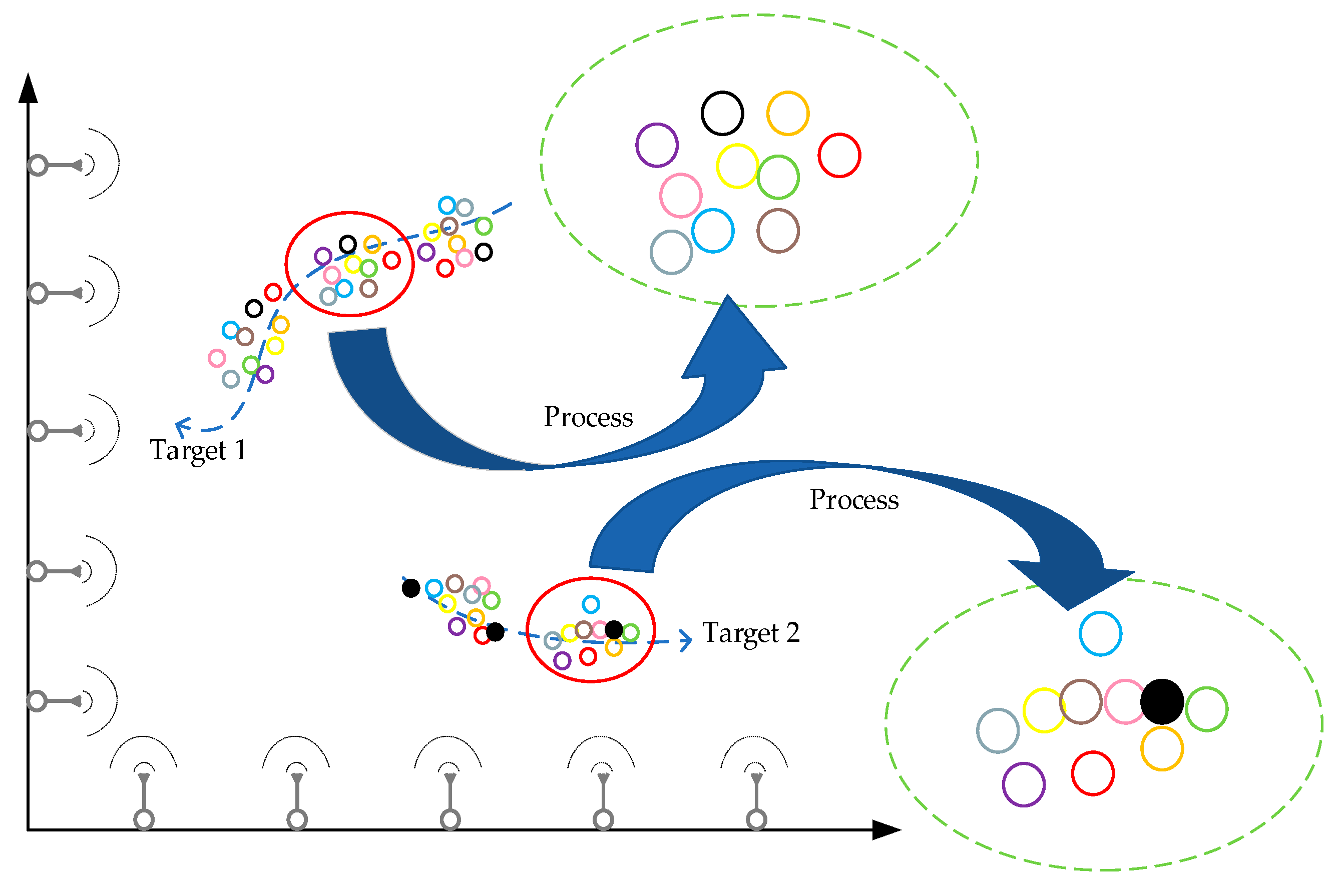
Before delving into the theoretical details of the algorithm, we provide a brief overview of its operation. It is important to note that although only the trajectories of two targets are illustrated in the figure for clarity (blue dashed lines), the actual application scenario of the proposed algorithm involves many more targets. As shown in Figure 1, points of different colors represent detections from various sensors, with each color corresponding to a different sensor source. For target 1, due to differences in the initial reporting times and reporting rates of each sensor, the data exhibit asynchrony in the temporal domain and positional deviations in the spatial domain caused by measurement errors. Considering the real-time requirements of the proposed algorithm and the definition of the distance metric, the earliest track point we can select for evaluation is the second reported point. For a global and fair comparison, we choose the latest time at which the second point is produced among all sensors as the reference time for data processing. The specific definitions and steps of the algorithm will be detailed in the following sections. For target 2, we treat the black solid points as a special case, where the reporting speed of the corresponding sensor is significantly faster than that of the other sensors. Therefore, we select the third solid point as the association object. This choice is based not on spatial proximity to the second point cluster, but on its reporting time being the closest to the chosen reference time. Furthermore, our algorithm is based on the association between individual measurement points, since each track point is tagged with both a target and a sensor identifier, meaning that every track point uniquely corresponds to one target and one sensor.

The algorithm proposed in this paper is based on sensor data, meaning that it can only be applied to track association in complex environments after target detection has been completed and the number of targets is known.

3.1. Definitions

Definition 1. 

Temporal Anchor.

Assuming M sensors simultaneously initiate detection of the same target area at time zero, the first two measurement points of each trajectory are obtained:

$$Tr(2)=\left[\begin{array}{c}{\Gamma }_1(\le 2)\\ {\Gamma }_2(\le 2)\\ ⋮\\ {\Gamma }_M(\le 2)\end{array}\right]=\left[\begin{array}{c}\{T_1^1,T_1^2,\cdots ,T_1^{N_1}\}(\le 2)\\ \{T_2^1,T_2^2,\cdots ,T_2^{N_2}\}(\le 2)\\ ⋮\\ \{T_M^1,T_M^2,\cdots ,T_M^{N_M}\}(\le 2)\end{array}\right]$$

(2)

where:

$$\{T_S^1,T_S^2,\cdots ,T_S^{N_1}\}(\le 2)=\left\{\begin{array}{cccc}\left[\begin{array}{c}{\xi }_S^{1,1}\\ {\xi }_S^{1,2}\end{array}\right]& \left[\begin{array}{c}{\xi }_S^{2,1}\\ {\xi }_S^{2,2}\end{array}\right]& \cdots & \left[\begin{array}{c}{\xi }_S^{N_s,1}\\ {\xi }_S^{N_s,2}\end{array}\right]\end{array}\right\}$$

(3)

The maximum value in Tr(2) is the temporal anchor $t_c$.

The concept of the temporal anchor is metaphorically derived from vessel anchoring. While physical anchoring fixes a ship’s spatial position, our temporal anchor establishes a fixed reference point in the time dimension. Subsequently, a step-2 temporal neighborhood affinity matrix is generated based on this temporal anchor.

Definition 2. 

Step-2 Temporal Neighborhood Affinity Matrix under Non-Registration Framework, STNAM.

Let M sensors with asynchronous reporting cycles (maximum reporting period $T_{max}$), and the STNAM D is defined as:

$$D={\left[\begin{array}{cccccccc}{\left({\xi }_1^{1,{\alpha }_1}\right)}^T& {\left({\xi }_1^{2,{\alpha }_2}\right)}^T& {\left({\xi }_1^{3,{\alpha }_3}\right)}^T& \cdots & {\left({\xi }_2^{1,{\alpha }_{N_1+1}}\right)}^T& \cdots & {\left({\xi }_M^{1,{\alpha }_{N_1+N_2+\cdots +N_{M-1}+1}}\right)}^T& \cdots \end{array}\right]}_{\left({\displaystyle \sum _i^M{N}_i}\right)\times 5}^T$$

(4)

where $0\text{<}{\alpha }_i\le \max \{N_1,N_2,\cdots ,N_M\}$ and $|t_S^{i,j}-t_c|\le T_{\max }$.

Notably, when multiple timestamped feature values $t_S^{i,j_1},t_S^{i,j_2}$ simultaneously satisfy the spatiotemporal constraints in matrix D, only the value closest to the reference time $t_c$ is retained for inclusion in the STNAM. That is, the STNAM is composed of feature vectors corresponding to the nearest track points at each reporting timestamp within individual trajectories. In this matrix, each row vector represents the features of a selected track point. Distinct rows either originate from different sensors or correspond to different detected targets. The subsequent execution of the SAS-KNN-DPC algorithm operates precisely on such a matrix. It can be seen that the construction of this matrix does not require time registration, and data preprocessing can be performed directly on data reported asynchronously by distributed networked sensors. In essence, the asynchrony problem is equivalent to the problem of missing data, as there may be no eligible points available for association at a certain moment or within a certain time period. Therefore, handling the asynchrony problem is to some extent also a discussion of track association under conditions of missing data.

Definition 3. 

K-Nearest Neighbors, KNN.

Given a distance metric $\rho$, a predefined integer $K$, and a dataset X, $\forall x_i\in X$, the K-nearest neighbors of $x_i$ are defined as the top $K$ samples in X with the smallest distances to $x_i$ under metric $\rho$. The set of these points is denoted as:

$$\mathrm{KNN}(x_i)=\left\{x_j\right|\rho (x_i,x_j)\le {\rho }_K\hspace{0.33em},\hspace{0.33em}\hspace{0.33em}{x}_i\ne x_j,\hspace{0.33em}\hspace{0.33em}{x}_j\in X\}$$

(5)

where ${\rho }_K$ denotes the K-th distance in the sorted distance sequence.

Definition 4. 

Multi-Feature Track-Point Fusion Similarity, simi.

Consider M sensors monitoring N targets within the same surveillance region, generating an STNAM D. Given the sensors’ maximum slant range measurement error $r_e$ and the targets’ maximum possible velocity $v_{\max }$, the multi-feature similarity between any two track points ${\xi }_{S_1}^{i\text{\_}1,j\text{\_}1}$ and ${\xi }_{S_2}^{i\text{\_}2,j\text{\_}2}$ (simi) is defined as:

$$\mathrm{simi}({\xi }_{S_1}^{i\text{\_}1,j\text{\_}1},{\xi }_{S_2}^{i\text{\_}2,j\text{\_}2})={\displaystyle \frac{1}{r_e+\mathrm{dist}({\xi }_{S_1}^{i\text{\_}1,j\text{\_}1},{\xi }_{S_2}^{i\text{\_}2,j\text{\_}2})}}+{\displaystyle \frac{1}{360+|{\theta }_{S_1}^{i\text{\_}1,j\text{\_}1}-{\theta }_{S_2}^{i\text{\_}2,j\text{\_}2}|}}+{\displaystyle \frac{1}{v_{\max }+|v_{S_1}^{i\text{\_}1,j\text{\_}1}-v_{S_2}^{i\text{\_}2,j\text{\_}2}|}}$$

(6)

$$\mathrm{dist}({\xi }_{S_1}^{i\text{\_}1,j\text{\_}1},{\xi }_{S_2}^{i\text{\_}2,j\text{\_}2})=\sqrt{{(x_{S_1}^{i\text{\_}1,j\text{\_}1}-x_{S_2}^{i\text{\_}2,j\text{\_}2})}^2+{(y_{S_1}^{i\text{\_}1,j\text{\_}1}-y_{S_2}^{i\text{\_}2,j\text{\_}2})}^2}$$

(7)

where ${\xi }_{S_1}^{i\text{\_}1,j\text{\_}1}$ denotes the feature vector of the j_1-th track point from the i_1-th track of sensor S₁, and ${\xi }_{S_2}^{i\text{\_}2,j\text{\_}2}$ is defined analogously.

Although the definition of simi appears to be a simple summation, the denominator parameter selection is critical. We choose the maximum possible value of each parameter as the parameter in the denominator, preventing disproportionate weighting in simi caused by extreme parameter magnitudes.

Definition 5. 

Multi-Feature Track-Point Fusion Similarity Matrix, MTFSM.

Consider M sensors monitoring N targets within the same surveillance region. Calculate the simi between all pairwise feature vectors in STNAM and construct a symmetric matrix of dimension $({\displaystyle \sum _{i=1}^M{N}_i)\times }({\displaystyle \sum _{i=1}^M{N}_i)}$.

$$\begin{array}{l}S={[s_{ij}]}_{N_M\times N_M}\\ \hspace{1em}=\left[\begin{array}{cccc}\mathrm{simi}({\xi }_1^{1,{\alpha }_1},{\xi }_1^{1,{\alpha }_1})& \mathrm{simi}({\xi }_1^{1,{\alpha }_1},{\xi }_1^{2,{\alpha }_2})& \cdots & \mathrm{simi}({\xi }_1^{1,{\alpha }_1},{\xi }_M^{N_M,{\alpha }_{N_1+N_2+\cdots +N_M}})\\ \mathrm{simi}({\xi }_1^{2,{\alpha }_2},{\xi }_1^{1,{\alpha }_1})& \mathrm{simi}({\xi }_1^{2,{\alpha }_2},{\xi }_1^{2,{\alpha }_2})& \cdots & \mathrm{simi}({\xi }_1^{2,{\alpha }_2},{\xi }_M^{N_M,{\alpha }_{N_1+N_2+\cdots +N_M}})\\ ⋮& ⋮& & ⋮\\ \mathrm{simi}({\xi }_M^{N_M,{\alpha }_{N_1+N_2+\cdots +N_M}},{\xi }_1^{1,{\alpha }_1})& \mathrm{simi}({\xi }_M^{N_M,{\alpha }_{N_1+N_2+\cdots +N_M}},{\xi }_1^{2,{\alpha }_2})& \cdots & \mathrm{simi}({\xi }_M^{N_M,{\alpha }_{N_1+N_2+\cdots +N_M}},{\xi }_M^{N_M,{\alpha }_{N_1+N_2+\cdots +N_M}})\end{array}\right]\end{array}$$

(8)

Definition 6. 

KNN-based Local Density Matrix, LD.

Given an MTFSM, the LD matrix is generated by performing descending sorting on each row and computing the sum of the first K values.

$$\begin{array}{c}LD={\left[\begin{array}{cccc}l{d}_1& l{d}_2& \cdots & l{d}_{N_1+N_2+\cdots +N_M}\end{array}\right]}^T\\ \hspace{1em}\hspace{1em}\hspace{1em}\hspace{1em}\hspace{1em}\hspace{1em}\hspace{1em}\hspace{1em} ={\left[\begin{array}{cccc}\mathit{ld}({\xi }_1^{1,{\alpha }_1})& \mathit{ld}({\xi }_1^{2,{\alpha }_2})& \cdots & \mathit{ld}({\xi }_M^{N_M,{\alpha }_{N_1+N_2+\cdots +N_M}})\end{array}\right]}^T\end{array}$$

(9)

$$\left\{\begin{array}{l}\hspace{1em}\mathit{ld}({\xi }_S^{i,j})=\max {\displaystyle \sum _{j=1}^{N_1+N_2+\cdots +N_M}{a}_j{s}_{i\prime j}}\\ {\displaystyle \sum _{j=1}^{N_1+N_2+\cdots +N_M}{a}_j=K}\\ \hspace{1em}\hspace{1em}{a}_j=0\hspace{0.33em}\mathit{or}\hspace{0.33em}1\end{array}\right.$$

(10)

Definition 7. 

Multi-Feature Step-2 Normalized Distance Matrix, MSNDM.

Given a similarity matrix $S_0$ derived from a specified metric function, the multi-feature step-2 normalized distance matrix $D_n$ is defined as:

$$D_n={(1-{(S_0./\max (S_0(:)))}^{0.1})}^{0.8}+0.00001$$

(11)

where $\max (S_0(:))$ denotes the maximum value in matrix $S_0$ and the constant 0.0001 prevents the maximum element in S₀ from becoming zero after normalization, ensuring numerical stability for subsequent computations. The larger the value, the farther the distance.

Definition 8. 

Global Relative Distance.

Given an STNAM D and its corresponding $LD$, each row (feature vector) in $D$ possesses a global relative distance. For the i-th row, its global relative distance ${\delta }_i$ is defined as:

$${\delta }_i=\underset{LD(i)<LD(j)}{\min }{D}_n(i,j)$$

(12)

Definition 9. 

Decision Value.

Consider M sensors monitoring N targets within the same surveillance region and setting the number of cluster centers K = N, the decision value of the i-th point is computed as:

$${\gamma }_i=l{d}_i\times {\delta }_i$$

(13)

Based on the computed ${\gamma }_i$ values, the largest K values are selected as cluster centers. In practice, each cluster center corresponds to one physical target, and correctly formed clusters represent detection of the same target by different sensors.

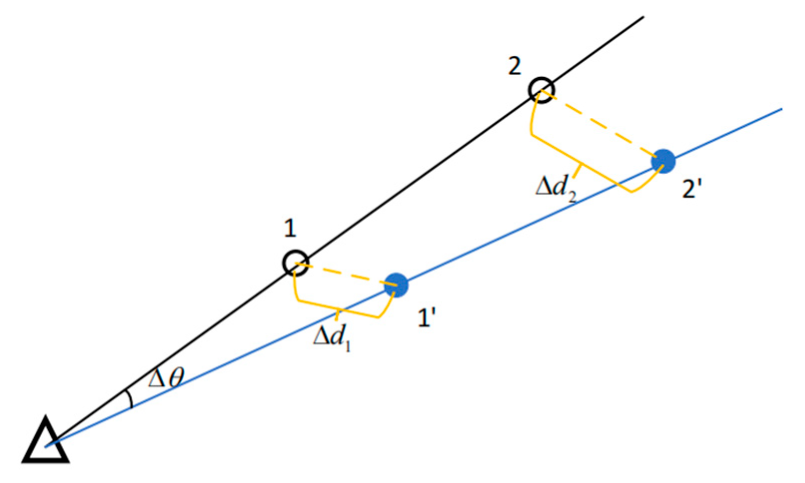
3.2. Self-Adaptive Step-2 Truncation Distance

The Hausdorff distance is a classical trajectory similarity metric for periodically batched tracks with accumulated points. The Hausdorff distance is defined as the maximum of all nearest-neighbor distances between two datasets, which captures their global shape similarity without requiring identical point counts or uniform sampling rates. This metric demonstrates particular robustness by maintaining stable similarity evaluation, even with partially missing data or noise contamination. Given two tracks $T_S^i,T_S^j(i,j=1,2,\cdots ,N_S)$, their Hausdorff distance is defined as:

$$hau(T_S^i,T_S^j)=\underset{{\xi }_S^{i,\alpha }\in T_S^i}{\max }\{\underset{{\xi }_S^{j,\beta }\in T_S^j}{\min }\{\mathrm{dist}({\xi }_S^{i,\alpha },{\xi }_S^{j,\beta })\}\}$$

(14)

where ${\xi }_S^{i,\alpha }=[t_S^{i,\alpha },x_S^{i,\alpha },y_S^{i,\alpha },{\theta }_S^{i,\alpha },v_S^{i,\alpha }]$ and ${\xi }_S^{i,\beta }=[t_S^{i,\beta },x_S^{i,\beta },y_S^{i,\beta },{\theta }_S^{i,\beta },v_S^{i,\beta }]$.

$\mathrm{dist}({\xi }_S^{i,\alpha },{\xi }_S^{j,\beta })$ represents the Euclidean distance between two vectors, with the specific expression given by:

$$\mathrm{dist}({\xi }_S^{i,\alpha },{\xi }_S^{j,\beta })=\sqrt{{(x_S^{i,\alpha }-x_S^{j,\beta })}^2+{(y_S^{i,\alpha }-y_S^{j,\beta })}^2}$$

(15)

The Hausdorff distance focuses on global shape matching, but cannot effectively capture local similarities or differences between trajectories. This metric is inapplicable for measuring similarity between individual track points. Based on this analysis, we propose a self-adaptive step-2 truncation distance that exclusively considers positional distances between track points while deliberately excluding heading and velocity information. We posit that only when the distance between track points in STNAM is smaller than the self-adaptive step-2 truncation distance can these points qualify for MTFS. Conversely, if the positional distance between two points exceeds the self-adaptive step-2 truncation distance, they are deemed irrelevant with zero similarity.

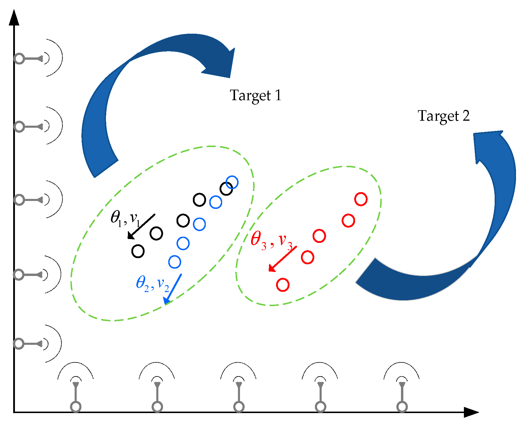
Since the similarity metric incorporates position, heading, and velocity information of track points, a special case occurs when two tracks are far apart, as shown in Figure 1.

The proposed algorithm operates on STNAM and does not require processing the full set of the whole track points. However, Figure 2 displays additional track points to better illustrate this special case. The three tracks are distinctly represented using black, blue, and red with corresponding labels 1, 2, and 3 respectively. Assuming track 1 and track 2 originate from the same target, they exhibit close spatial proximity, but significant discrepancies in heading and velocity due to measurement errors. Track 1 and track 3 originate from distinct targets, exhibiting significant spatial separation, but minimal differences in heading and velocity parameters. Consequently, according to Equation (6), it becomes challenging to determine whether track 2 or 3 should be associated with track 1. In light of this consideration, this paper proposes the concept of self-adaptive step-2 truncation distance. Track points qualify for both kinematic and positional feature comparison only if their positional distance is smaller than the self-adaptive step-2 truncation distance. Points beyond this threshold are considered uncorrelated, and their spatial relationship is fundamentally invalid. More fundamentally, it is emphasized that the step-truncation distance must be adaptively generated rather than manually specified, enabling autonomous determination of optimal truncation boundary based on the intrinsic distribution characteristics of the reported data.

Definition 10. 

Self-Adaptive Step-2 Truncation Distance.

Consider M sensors monitoring N targets within the same surveillance region. In the STNAM, for data originating from the same sensor (denoted as the S-th sensor) $\{{\xi }_S^{1,{\alpha }_{\beta +2}},{\xi }_S^{2,{\alpha }_{\beta +2}},{\xi }_S^{3,{\alpha }_{\beta +3}},\cdots ,{\xi }_S^{N_S,{\alpha }_{\beta +N_S}}\}(\beta =N_1+N_2+\cdots +N_{S-1})$, obtain the largest distance value $d_{\max \text{\_}S}$:

$$d_{\max \text{\_}S}=\underset{S}{\max } \underset{i\ne j}{\min }(\mathrm{dist}({\xi }_S^{i,\omega },{\xi }_S^{j,\psi }))$$

(16)

Definition 11. 

Self-Adaptive Multi-Feature Similarity Truncation Matrix, SMSTM.

Given an MTFSM and its corresponding SASTD, for any element simi (a, b), $a,b\in \{{\xi }_1^{1,{\alpha }_1},{\xi }_1^{2,{\alpha }_2},{\xi }_1^{3,{\alpha }_3},\cdots ,{\xi }_M^{1,{\alpha }_{N_1+N_2+\cdots +N_M}},\cdots \}$, if:

$$\mathrm{dist}(a,b)>d_{\max \text{\_}S}$$

(17)

then simi (a, b) = 0, and the self-adaptive multi-feature similarity truncation matrix F is formed:

$$F=\left[\begin{array}{cccc}\chi \left(\mathrm{dist}\right({\xi }_1^{1,{\alpha }_1},{\xi }_1^{1,{\alpha }_1})-d_{\max \text{\_}S})s_{11}& \chi \left(\mathrm{dist}\right({\xi }_1^{1,{\alpha }_1},{\xi }_1^{2,{\alpha }_2})-d_{\max \text{\_}S})s_{11}& \cdots & \chi \left(\mathrm{dist}\right({\xi }_1^{1,{\alpha }_1},{\xi }_M^{N_M,{\alpha }_{N_t}})-d_{\max \text{\_}S})s_{11}\\ \chi (\mathrm{dist}({\xi }_1^{2,{\alpha }_2},{\xi }_1^{1,{\alpha }_1})-d_{\max \text{\_}S})s_{21}& \chi \left(\mathrm{dist}\right({\xi }_1^{2,{\alpha }_2},{\xi }_1^{2,{\alpha }_2})-d_{\max \text{\_}S})s_{22}& \cdots & \chi \left(\mathrm{dist}\right({\xi }_1^{2,{\alpha }_2},{\xi }_M^{N_M,{\alpha }_{N_t}})-d_{\max \text{\_}S})s_{2N_t}\\ ⋮& ⋮& & ⋮\\ \chi (\mathrm{dist}({\xi }_M^{N_M,{\alpha }_{N_t}},{\xi }_1^{1,{\alpha }_1})-d_{\max \text{\_}S})s_{N_{t}1}& \chi \left(\mathrm{dist}\right({\xi }_M^{N_M,{\alpha }_{N_t}},{\xi }_1^{2,{\alpha }_2})-d_{\max \text{\_}S})s_{N_{t}2}& \cdots & \chi \left(\mathrm{dist}\right({\xi }_M^{N_M,{\alpha }_{N_t}},{\xi }_M^{N_M,{\alpha }_{N_t}})-d_{\max \text{\_}S})s_{N_t{N}_t}\end{array}\right]$$

(18)

where $N_t=N_1+N_2+\cdots +N_M$ and:

$$\chi (x)=\left\{\begin{array}{c}1,\hspace{1em}x\text{<}0\\ 0,\hspace{1em}\mathrm{else}\hspace{0.33em}\end{array}\right.$$

(19)

The specific implementation steps for the aforementioned definitions can be found in the detailed algorithm framework and pseudocode described later.

3.3. The Framework of SAS-KNN-DPC Algorithm

The structural framework of the SAS-KNN-DPC algorithm, as illustrated in Figure 3, primarily comprises three key operational steps:

Step 1. (Track point similarity metric) For track points reported in real-time within the STNAM D, a similarity metric is applied. This utilizes the MTFSM along with the corresponding SASTD to generate SMSTM F.

Step 2. (Cluster center selection) The SMSTM F generates LD and global relative distance, which are subsequently used to compute decision values for cluster center determination. Each distinct cluster center represents a unique target.

Step 3. (Association assignment) By leveraging the K-nearest neighbor (KNN) relationships within the SMSTM F, each cluster center and its corresponding K-nearest neighbors form a complete cluster. Each cluster represents the collective detection of a single target across all sensors.

3.4. Similarity Metric

Nearly all existing association algorithms operate by exhaustively pairing all tracks between two sensors in a pairwise manner. In practical multi-sensor scenarios, this approach entails two levels of combinatorial complexity: first, all sensors must be paired combinatorially; and second, within each sensor pair, all reported tracks must again be matched pairwise. This dual-layer exhaustive search not only drastically increases computational overhead and reduces efficiency but also fails to meet real-time requirements. Furthermore, the core challenge of track association lies in defining the appropriate distance metric between tracks. Current metrics almost exclusively rely on accumulated track sequences, meaning that a period of track-point accumulation is required to enable inter-track distance measurement before association occurs. This inherent latency fundamentally conflicts with real-time processing demands. Our proposed algorithm addresses this problem by performing distance calculations directly on real-time track reports, eliminating the need for prolonged track accumulation prior to metric evaluation.

The whole similarity metric proposed in this paper utilizes two complementary distance metrics to achieve efficient track association. One calculates $d_{\max \text{\_}S}$ using purely positional information, while the other implements a multi-feature similarity measure incorporating kinematic attributes and positional data.

As previously discussed, we posit that in practical scenarios, when the positional distance between two track points exceeds $d_{\max \text{\_}S}$, the probability of them originating from the same target becomes statistically negligible. Consequently, further computation of their MTFS can be safely omitted.

Step 1. For real-time track reporting, temporal anchor t_c is extracted and STNAM is constructed. In STNAM, each row vector represents a sensor’s track-point observation of a target, and each column corresponds to a distinct feature parameter of the track points.

Step 2. The MTFS between each row is computed according to Equation (6), yielding MTFSM.

Step 3. Calculate the minimum Euclidean distance between any two track points reported by the i-th sensor. Then iterate through all sensors and select the maximum value among these minimum distances as $d_{\max \text{\_}S}$.

Step 4. Using the $d_{\max \text{\_}S}$, process matrix MTFSM by setting elements satisfying Equation (17) to zero, thereby generating matrix SMSTM F.

${\xi }_S^{i,j\prime }$ denotes the j’-th track point of the i-th track reported by the S-th sensor, where this point is selected as the one with a timestamp closest to the temporal anchor t_c among all points in this track. The operation $\mathrm{sum}(temp,2)$ computes row-wise summation of the temp.

3.5. Cluster Center Selection and Association Assignment

The detailed steps are as follows:

Line 11 implies not only assigning the maximum value to the cluster but also allocating the corresponding label (indicating which target from which sensor) to the cluster. Under normal circumstances, these targets are distinct from each other. Line 12 identifies the nearest neighbors corresponding to each cluster center in the F and assigns them to their respective cluster centers. Under nominal conditions, each cluster corresponds to a distinct target, with the cluster’s data originating from multiple sensors.

3.6. Time Complexity

We assume that M sensors are detecting N targets within the same surveillance region.

According to the previous section, the detailed analysis of Algorithm 1 is as follows.

Lines 2–7: For each track, the point closest to temporal anchor t_c must be extracted, which involves conditional logic (if-statements) and comparison operations, and complexity is O(MN).

Lines 8–13: Extract the track point closest to the anchored timestamp t_c from each track, requiring traversal of tracks. Thus, the complexity is O(MN).

Lines 14–18: Compute pairwise vector for elements in D using MTFS and the positional distance metric, resulting in O((MN)²).

Lines 19: The $d_{\max \text{\_}S}$ requires computing the row-wise summation of the matrix, and the complexity is O((MN)²).

Lines 20–26: Compute SMSTM. After satisfying the if-condition, each element in SMSTM requires value assignment, resulting in O((MN)²).

Algorithm 1 Compute SMSTM

Input: 1. The number of sensors

2. The number of targets

3. The second track points generated by each radar

Output: SMSTM

$1\text{:} C\leftarrow 0,D\leftarrow 0,S\leftarrow 0,\mathrm{label}\leftarrow 0,t_c\leftarrow 0$

$2\text{:} \mathbf{for} \mathrm{each} t_S^{i,j}$$\mathrm{in} Tr(2)$ do

$3\text{:}\hspace{1em}\hspace{1em}\mathbf{if} t_c\le t_S^{i,j}$ then

$4\text{:}\hspace{1em}\hspace{1em}\hspace{1em}{t}_c=t_S^{i,j}$$\mathrm{and} S\prime =S$$\mathrm{and} i\prime =i$

$5\text{:}\hspace{1em}\hspace{1em}\hspace{1em}\mathrm{label}=\left\{S\prime ,i\prime ,2\right\}$

6:  end if

7: end for

8: for each sensor $S$ do

$9\text{:}\hspace{1em}\hspace{1em}\mathbf{for} \mathrm{each} T_S^i$$\mathrm{in} {\Gamma }_S$ do

$10\text{:}\hspace{1em}\hspace{1em}\hspace{1em} \mathbf{if} |t_S^{i,j\prime }-t_c|\hspace{0.33em}\mathrm{is}\hspace{0.33em}\mathrm{the}\hspace{0.33em}\mathrm{maximum} \mathrm{among} \mathrm{all} \mathrm{the} |t_S^{i,j}-t_c|(1\le j\le N_S^i)$ then

$11\text{:}\hspace{1em}\hspace{1em}\hspace{1em}\hspace{1em} D\leftarrow [D;{\xi }_S^{i,j\prime }]$

12:  end for

13: end for

14: for each i and j in row($D$) do

$15\text{:}\hspace{1em}\hspace{1em} S(i,j)\leftarrow \mathrm{simi}(D(i),D(j))$$\mathrm{and} \mathit{temp}(i,j)\leftarrow \mathrm{sqrt}(D(i),D(j))$

16:  end for

17: end for

$18\text{:} d_{\max \text{\_}S}\leftarrow \min (\mathrm{sum}(\mathit{temp},2))$

19: for each i in row($S$) do

20:  for each j in col($S$) do

$21\text{:}\hspace{1em}\hspace{1em}\hspace{1em}\mathbf{if} \mathrm{sqrt}(D(i),D(j))\ge d_{\max \text{\_}S}$  then

$22\text{:}\hspace{1em}\hspace{1em}\hspace{1em}\hspace{1em}F(i,j)\leftarrow 0$

23:   end if

24: end for

25: end for

According to the previous section, the detailed analysis of Algorithm 2 is as follows.

Lines 2–5: Compute LD and the complexity is O(MN).

Lines 6: There are (MN)² elements in SMSTM, and the complexity is O(MN).

Lines 7–9: Compute the relative distance matrix by traversing each element in $D_n$, yielding a time complexity of O((MN)²).

Lines 10–12: All three steps involve numerical computations or comparisons, and the complexity is O((MN)²).

Algorithm 2 Cluster Formation

Input: 1. The number of sensors

2. The number of targets

3. SMSTM

Output: Cluster

$1\text{:} C\leftarrow 0,K\leftarrow \mathit{num}\text{\_}r,\mathit{temp}\text{\_}1\leftarrow 0,LD\leftarrow 0,D\leftarrow 0,\Theta \leftarrow 0,H\leftarrow 0$

2: for each i in row($F$) do

$3\text{:}\hspace{1em} \mathit{temp}\text{\_}1\leftarrow$$\mathrm{sort} F(\text{:},K)$ in descending order

$4\text{:}\hspace{1em} LD(i)\leftarrow \mathrm{sum}(\mathit{temp}\text{\_}1)$

5: end for

$6\text{:}\hspace{1em}{D}_n={(1-{(F./\max (F(\text{:})))}^{0.1})}^{0.8}+0.00001$

$7\text{:} \mathrm{for} \mathrm{each} i \mathrm{in} \mathrm{row}(D_n$) do

$8\text{:}\hspace{1em}\hspace{1em}\Theta (i)\leftarrow$$\underset{{\rho }_j\text{>}{\rho }_i}{\min }(D_n(i,j))$$\mathrm{with} j=1,2,\cdots ,\mathrm{col}(D_n)$

9: end for

$10\text{:} H\leftarrow \Theta .* LD$

$11\text{:} C\leftarrow$ select the top $K$ largest values

$12\text{:} C\leftarrow$ KNN based on $F$

3.7. Space Complexity

STNAM contains features of track points with O(MN) space complexity. The system involves M heterogeneous sensors monitoring N targets within a common surveillance region, where each sensor generates tracks of varying lengths. For each trajectory, select the track point with the reporting timestamp closest to t_c to participate in clustering operations. The space complexity of matrices $S,F,D_n$ is O((MN)²), while that of $LD,\Theta ,H,C$ is O(MN).

4. Experiments

4.1. Simulation Scene Setting

The experimental validation was conducted using simulated spatiotemporal track data. We assume multiple sensors simultaneously detect all targets within a common surveillance region and generate corresponding measurements. Real-time association is performed on these track data. The experimental design process and results are discussed in detail. The simulation environment is a 64-bit Windows 10 operating system and the MATLAB R2024 software platform. The processor is an Intel(R) Core(TM) i7-7700HQ with a main frequency of 2.80 GHz.

4.1.1. Scenario Data Visualization Analysis

The trajectory generation program published by Piciarelli et al. has been widely used in simulation studies for trajectory classification algorithms [39]. This program can generate random anomalous trajectories, set the number of trajectory clusters, and configure trajectory distribution parameters according to simulation requirements, including the number of information points per trajectory and the quantity of anomalous trajectories [29]. It serves as an effective validation tool for both anomaly detection and multi-trajectory clustering algorithms. In this section, based on this trajectory generation program, we extracted and modified part of its data while adding parameters such as heading, speed, and operational range to the information points, aiming to create irregular and unpredictable flight trajectories. 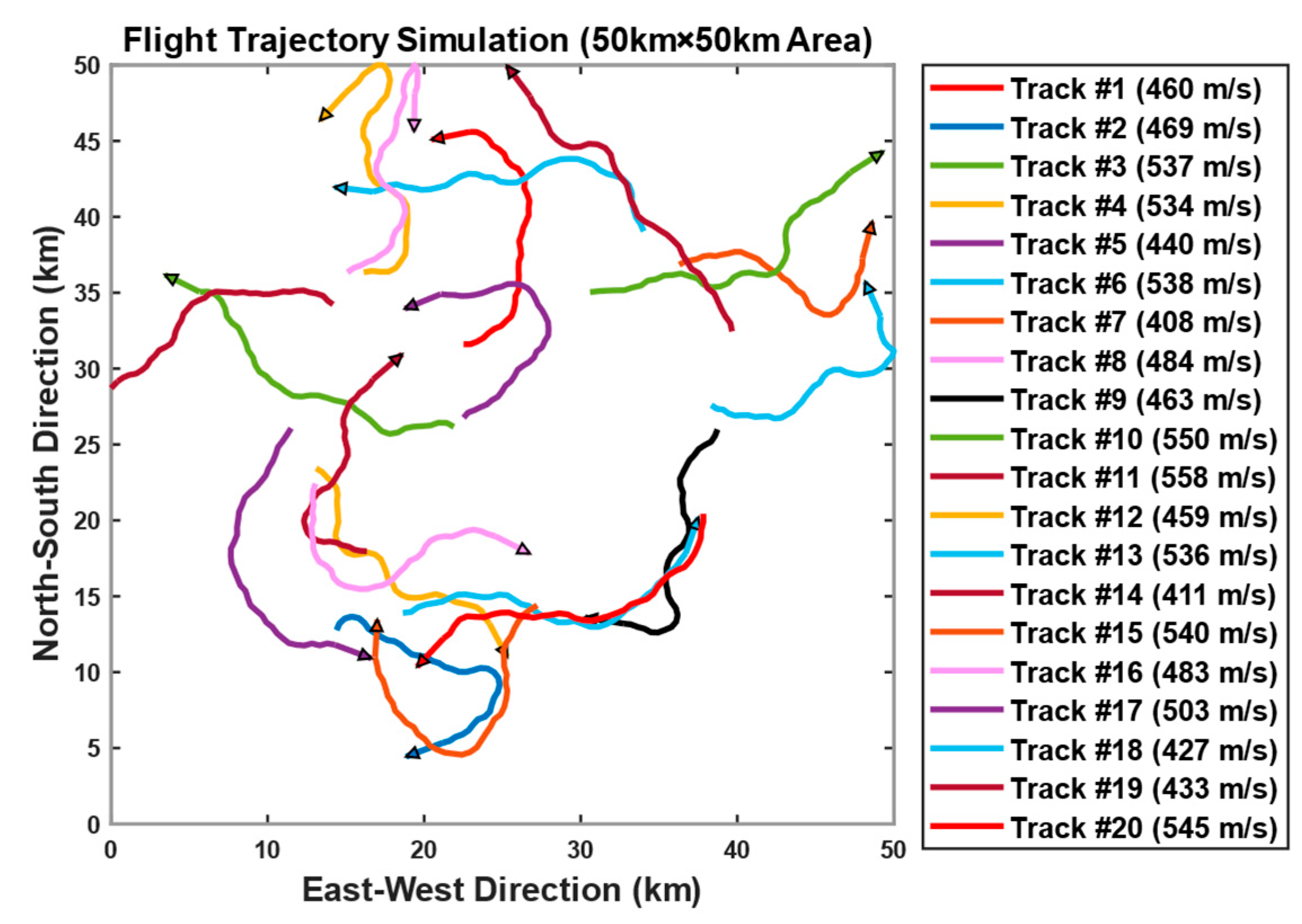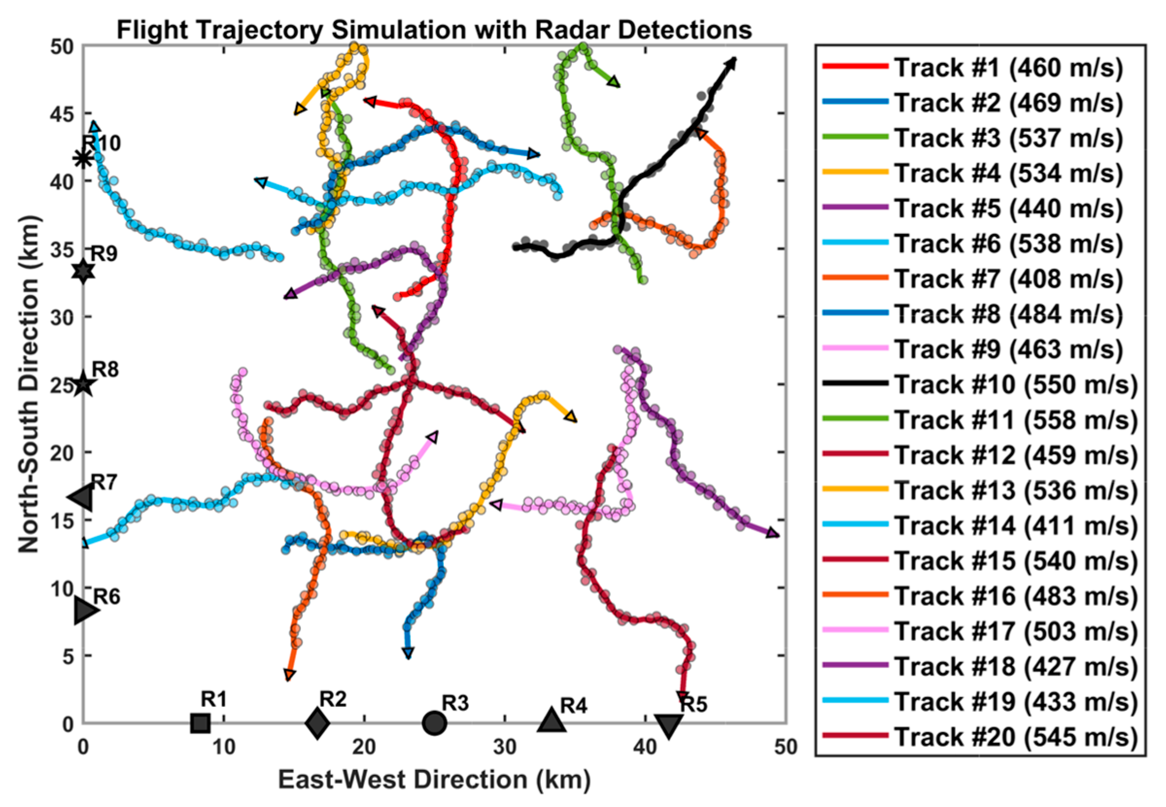Figure 4 shows a schematic diagram of 20 tracks.

The specific information of these tracks is shown below. Twenty tracks were generated within the designated area $x\in [0\hspace{0.33em}\mathrm{km},\hspace{0.33em}50\hspace{0.33em}\mathrm{km}],\hspace{0.33em}y\in [0\hspace{0.33em}\mathrm{km},\hspace{0.33em}50\hspace{0.33em}\mathrm{km}]$, with the initial headings of the targets following a uniform distribution between 0 and 360 degrees. The target velocities follow a uniform distribution ranging from 400 m/s to 600 m/s and the maximum turning rate is 30 degrees per second. It is essential to specify the operational area of tracks because during simulation verification, the impact of sensor slant range measurement errors and angular measurement errors on track association results varies with the target distance. Under identical sensor measurement errors, the detection error increases with target distance, as illustrated in Figure 5.

Black hollow points represent the true positions of targets, while blue solid points denote the measured positions. Target 1 and target 2 are aligned along the same azimuth angle of the sensor, but differ in range. Under identical measurement errors, the positional deviations between true and measured positions are $\Delta d_1,\hspace{0.33em}\Delta d_2$ for the two targets respectively. As expected, target 2, at greater sensor range, exhibits larger measurement deviation. This illustrates the measurement deviation of a single target relative to a single sensor. For multi-target multi-sensor scenarios, the operational area boundaries must be explicitly defined in simulations and the impact of the target distance will be studied further in the subsequent section.

The track association problem fundamentally processes sequences of track points. For visualization purposes, Figure 6 demonstrates the simulation results incorporating sensor detection effects. The circular plots in the diagram represent simulated track points with measurement errors added. The simulation configures ten radar coordinates uniformly distributed along the x and y axes.

4.1.2. Experimental Design

Association accuracy and real-time performance are the two most critical advantages of the proposed track association algorithm, which also constitute the primary focus of simulation validation. We apply the proposed algorithm to this simulated tracks, and the details of the experimental projects and design concepts are outlined as follows.

Set the situation in Figure 6 as scenario 1, with the number of targets, initial headings, target velocities, and turn rates consistent with the Figure 4 scenario. The number of radars is set to 10, uniformly distributed along the x and y axes. The total observation time is 5 s. Specific parameters are listed in

Table 1. The parameter settings of radars.

Contents	Ranges
Radar data reporting cycle (s)	[0.1, 1.2]
Azimuth measurement error (°)	[−0.3, 0.3]
Range measurement error (m)	[−100, 100]
Time of the initial data report (s)	[0, 1.2]

.

(1)

To validate the association accuracy of the proposed algorithm, comparative experiments with other methods are conducted under scenario 1, while varying error parameters to rigorously evaluate the algorithm’s performance.

(2)

To validate the real-time performance of the proposed algorithm, scenario 1 is modified by varying the number of targets from 10 to 100 (in increments of 10). Comparative experiments are conducted against other existing algorithms.

(3)

To validate sensor scalability and operational applicability, scenario 2 is configured by dynamically adjusting the number of sensors (baseline: 10) in scenario 1. The sensor count is varied from 6 to 30.

(4)

To validate the impact of target distance on the accuracy of the algorithm proposed, an analysis is conducted by varying the target activity range.

4.2. Experiment Based on Scenario 1

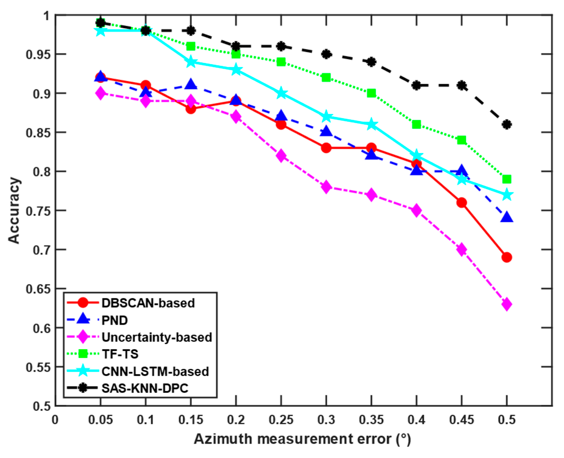
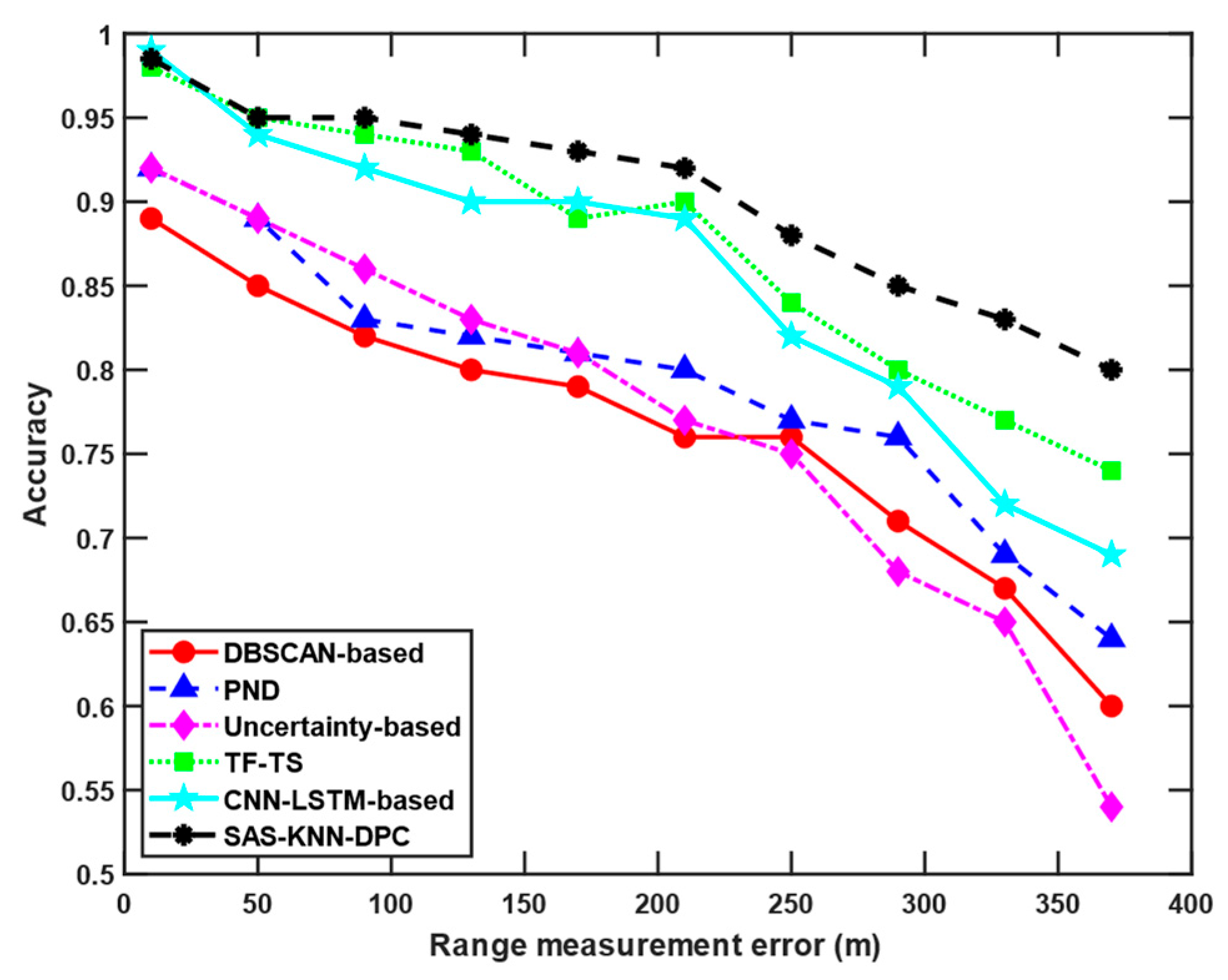
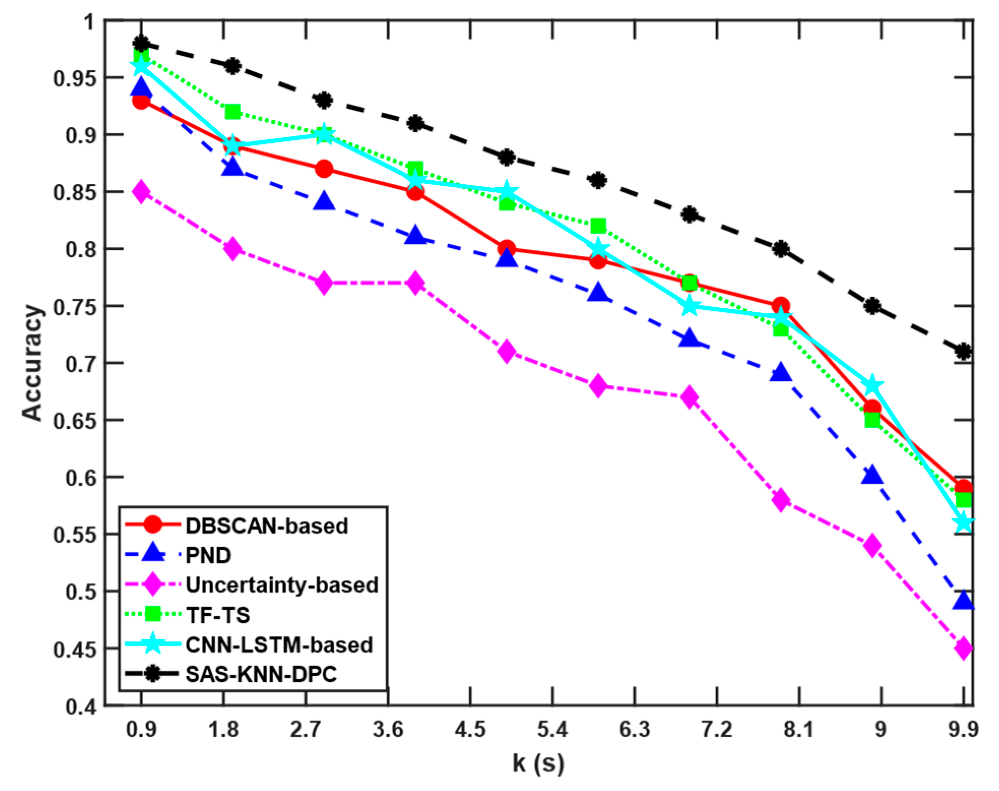
To demonstrate the feasibility and superiority of the proposed algorithm, comparative experiments are conducted under scenario 1, focusing on two key factors: association accuracy and real-time performance. The proposed method is evaluated against five novel algorithms: DBSCAN-based [27], PND [40], uncertainty-based [41], TF-TS [26], and CNN-LSTM-based algorithms [42].

To ensure the reliability and superiority of the experimental results, each algorithm was tested 1000 times (these 1000 experiments were divided into groups of 100 experiments each, and the association accuracy is calculated for every group). The track scenarios were generated using the rng( ) random seed function in MATLAB, allowing for precise control of a single variable while maintaining randomness in the distribution of scenarios.

In randomly generated trajectories, there exist overlapping/crossing trajectories and those in close proximity, which significantly impact association accuracy. However, most randomly generated tracks are non-intersecting and well separated. If only the mean association accuracy is used as the evaluation metric, it would fail to comprehensively reflect the effectiveness and robustness of the track association algorithm. Therefore, this study establishes the following four evaluation parameters for systematic comparative analysis:

• Worst association accuracy, reflecting the algorithm’s performance lower bound in extreme scenarios.
• Best association accuracy, demonstrating the algorithm’s potential under ideal conditions.
• Mean value, representing the overall average performance.
• Variance value, quantifying stability and consistency.

The variance indicates the stability of different algorithms when dealing with various random tracks, and the mean value represents the general performance of each algorithm. As shown in

Table 2. Association results of contrast experiments.

Contents	Worst Association Accuracy	Best Association Accuracy	Mean	Variance (×10−4)
DBSCAN-based	0.81	0.86	0.835	3.3778
PND	0.78	0.84	0.81	5.5111
Uncertainty-based	0.75	0.83	0.79	5.6556
TF-TS	0.85	0.96	0.905	2.8444
CNN-LSTM-based	0.87	0.95	0.910	2.4733
SAS-KNN-DPC (ours)	0.92	0.99	0.955	2.4800

, in addition to the algorithm proposed, TF-TS and CNN-LSTM-based algorithm demonstrate superior performance in terms of both association accuracy and stability. The former innovatively integrates a track fusion module and a track segmentation mapping module, autonomously extracting and synthesizing track features without reliance on empirical thresholds or heuristic assumptions. The latter employs a CNN-LSTM hybrid architecture, where the LSTM component specializes in capturing long-term temporal dependencies inherent in sequential data, while the CNN module efficiently processes localized short-term patterns. This synergistic combination enables comprehensive utilization of both long-range and short-range track features, with the final association decision generated through an integrated classifier. These two neural network-based AI algorithms exhibit strong adaptability, delivering better association accuracy and robust stability in performance. The DBSCAN-based algorithm is primarily designed for mechanical circular scanning scenarios and demonstrates limited effectiveness in handling asynchronous data processing tasks. The PND (pseudo-nearest-neighbor distance) method employs an innovative distance metric. This metric definition demonstrates suboptimal association performance and unstable behavior when applied to targets with proximity or intersecting tracks. The uncertainty-based algorithmic model is constructed under the idealized assumption of completed track point preprocessing, exhibiting limited adaptability to highly maneuvering target scenarios with notably higher variance and compromised stability. The proposed algorithm distinguishes itself from comparative methods by leveraging only the initial single-point trajectory measurements from each sensor for real-time data association. This approach circumvents the need for prolonged data accumulation to form complete tracks, thereby achieving more efficient information utilization while minimizing the accumulation of measurement errors. Consequently, the algorithm demonstrates significantly enhanced stability and accuracy in operational scenarios.

Figure 7 shows a comparative analysis of the accuracy achieved by different algorithms under identical scenarios, with varying angular measurement errors from 0° to 0.5°. The experimental results show that when the angular measurement error is small, the TF-TS, CNN-LSTM-based, and SAS-KNN-DPC algorithms all perform well with comparable association accuracy rates. However, as the angular measurement error increases, the accuracy of all algorithms declines, with a particularly noticeable drop when the error reaches 0.5°. Overall, the proposed SAS-KNN-DPC algorithm demonstrates superior accuracy compared to other methods in this study. However, it should be noted that the inherent randomness in target track generation may occasionally lead to counterintuitive association results. Specifically, in scenarios with randomly generated intersecting or adjacent tracks, smaller measurement errors may paradoxically yield lower association accuracy compared to cases with larger errors. This phenomenon, however, does not negate the fundamental influence of random measurement errors on association performance.

Similarly, Figure 8 compares the accuracy of different algorithms under identical scenario with varying distance measurement errors, and the angular measurement error is fixed at 0.3°. The slant range measurement error was systematically varied from 10 to 370 m. It can be observed that when the errors are small, the TF-TS, CNN-LSTM-based, and SAS-KNN-DPC algorithms all achieve relatively high accuracy.

The asynchronous problem of radar data association, caused by differences in reporting cycles and initial data timestamps, fundamentally impacts track matching by introducing time discrepancies. These timing variations lead to significant changes in target information and degraded association accuracy. The experimental configuration sets the shortest data reporting cycle among the ten radars to 0.1 s, while the longest reporting cycle varies uniformly between 1 s and 10 s. The parameter k is defined as the difference between the maximum and minimum reporting cycles. Each radar’s reporting cycle is then assigned a value uniformly spaced between these minimum and maximum bounds. Comparative results are presented in Figure 9.

As shown in Figure 9, as the value of k increases—indicating greater disparity in data reporting cycles among sensors—the asynchronous data reporting problem becomes more severe. Consequently, the accuracy rates of all algorithms exhibit an overall declining trend, which aligns with intuitive expectations. The DBSCAN-based algorithm utilizes the DBSCAN clustering method, which shares a similar innovative starting point with our proposed algorithm. Both approaches aim to mitigate the impact of temporal discrepancies in asynchronous data association to some extent through clustering techniques. However, this algorithm fails to consider the physical motion characteristics of targets, such as their heading direction and speed—crucial pieces of information for accurate association. Moreover, the DBSCAN clustering method has several inherent limitations: it heavily depends on parameter settings (making it less adaptive), performs poorly with manifold structures, and struggles with complex non-convex clusters. These limitations constitute significant factors that restrict the algorithm’s potential for further accuracy improvement. The PND algorithm focuses on addressing the track asynchrony issue. When the ratio of data reporting cycles between two sensors is less than 4, it achieves near-perfect accuracy (approaching 100%). However, when the number of sensors increases and asynchrony occurs among multiple sensors (not just between two or three), the algorithm’s accuracy drops significantly. In multi-sensor and multi-target scenarios, this method requires pairwise matching between both sensors and tracks, which substantially increases processing time for asynchronous data. As a result, its overall performance is poor. The TF-TS and CNN-LSTM-based algorithms leverage neural networks, offering adaptability and flexibility to extract key information and features from track sequences. These approaches demonstrate superior performance in handling asynchronous problems compared to the traditional algorithms; however, when significant asynchrony-induced temporal discrepancies exist in the data, all these algorithms demonstrate notable limitations in accuracy. The proposed SAS-KNN-DPC algorithm also exhibits adaptive capabilities because of the self-adaptive step-2 truncation distance proposed. More importantly, it can mitigate the impact of excessive asynchrony-induced data discrepancies to some extent through STNAM, and additionally incorporates target motion characteristics and imposes almost no requirements on temporal alignment, enabling it to overcome the challenges posed by temporal mismatches in asynchronous data. Consequently, it demonstrates optimal overall performance.

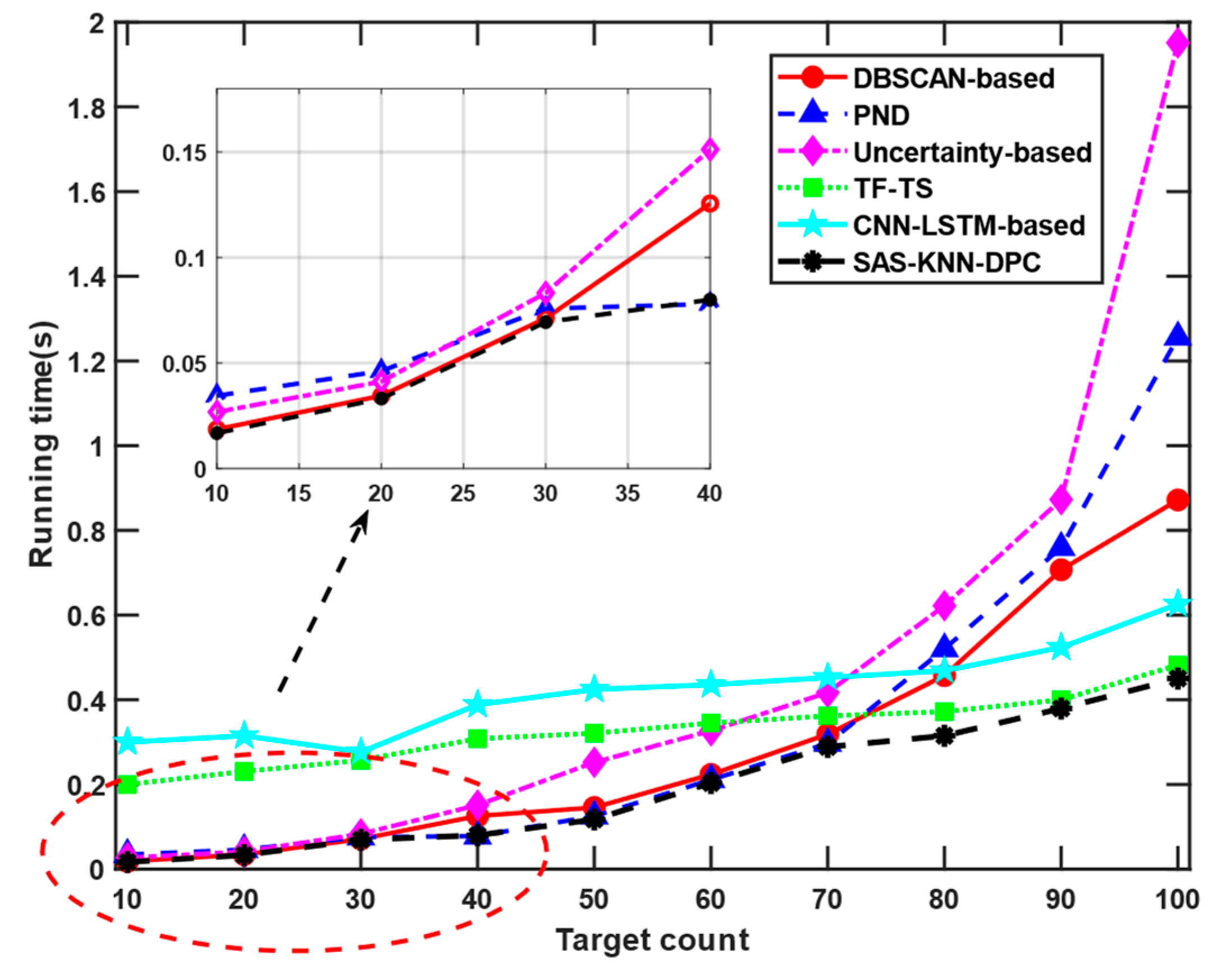
4.3. Real-Time Performance Verification

The real-time performance verification of the proposed algorithm encompasses two key processes: first, evaluating the time complexity of the algorithm itself while excluding track generation time; and second, assessing the complete end-to-end processing duration from data reporting to result output, which includes the actual data generation time. Currently, almost all track association algorithms process data based on sequences of track points. In other words, they first generate complete track data, and then determine whether two given tracks originate from the same target. The more track points are generated, the more operational data and references become available for track association, which may lead to higher accuracy rates in the association process. However, in the real-time simulation verification experiments, it was not feasible to reasonably configure the number of track points due to various constraints. From an intuitive perspective, the method proposed in this paper requires fewer reporting track points and shorter data acquisition time (for instance, generating two track points is faster than producing five track points). Therefore, in this context, only comparing the algorithms’ inherent computational time consumption yields meaningful results.

In scenario 1, excluding the time required for track data generation, we designate the moment when the target track data are ready for processing as the initial timestamp (t = 0) for algorithm verification, and proceed to analyze the algorithm’s execution time, as illustrated in Figure 10.

In scenario 1, starting the analysis with 10 targets, we observe that when the number of targets remains below 40, all algorithms except AI-based methods exhibit relatively low computational overhead. When the number of targets approaches or exceeds 40, the running time of all algorithms increases. Notably, our proposed algorithm consistently demonstrates the lowest computational overhead under these conditions. The uncertainty-based method consumes a certain amount of computation time for noise model construction and it also employs conventional mathematical statistical approaches, which incur computational overhead. The higher computational time of the PND algorithm is attributed to its reliance on pseudo-nearest-neighbor distance for track distance measurement. This method requires calculating the minimum distances between all trajectory points in both tracks and then selecting the maximum value from these computations, resulting in a relatively large computational load and longer processing time. When evaluating neural network-based algorithms, the computational cost must account for the substantial training time expenditure. Consequently, even with a limited number of targets, these algorithms exhibit prolonged execution durations due to their inherent training overhead. However, from a holistic perspective, the algorithm demonstrates both time-efficient and stable performance characteristics. To be specific, TF-TS transforms the track tensor of the tracks into association matrix directly, saving much consumption time.

From a global perspective, whether the target count is large or small, the proposed algorithm consistently maintains low running time. Further, when factoring in data reporting time, the advantages of the proposed algorithm become even more apparent, with STNAM processing.

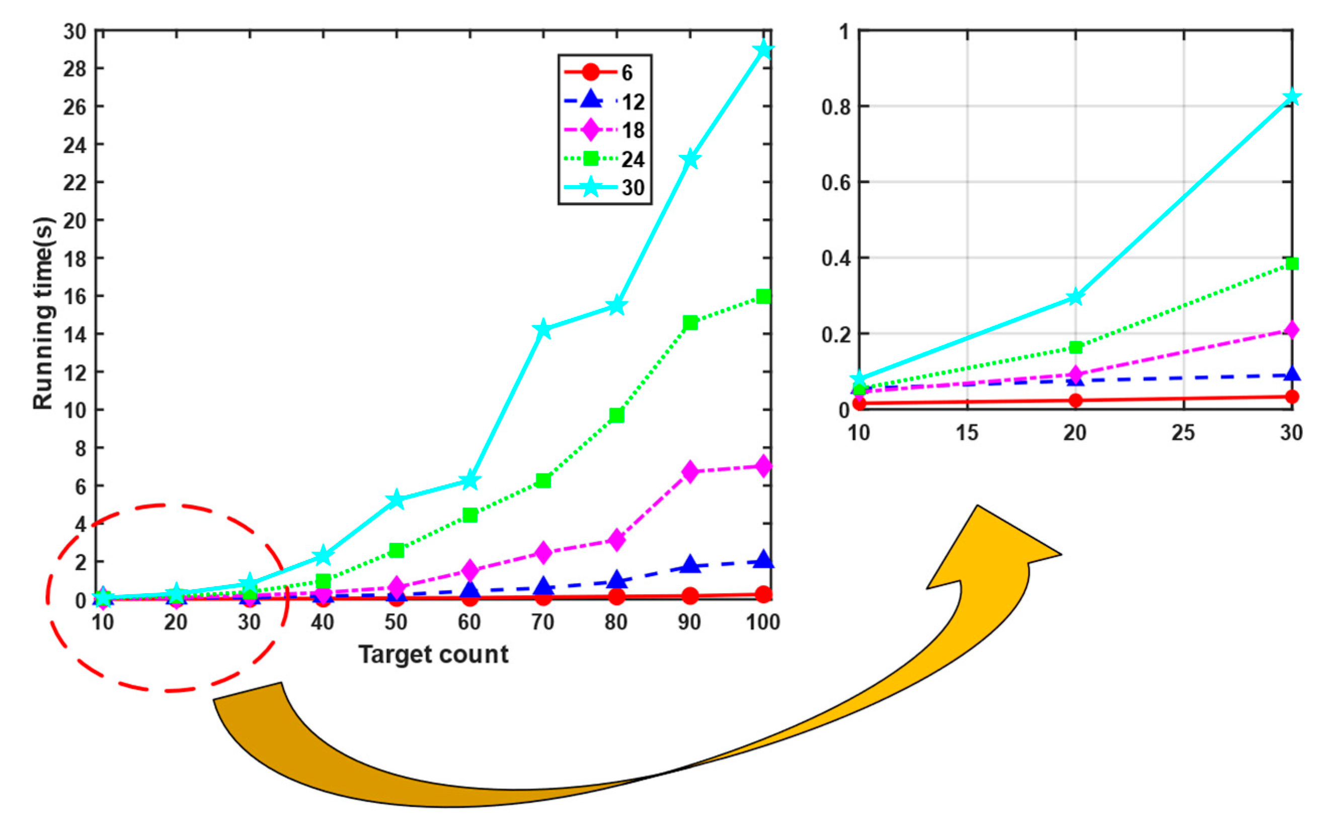
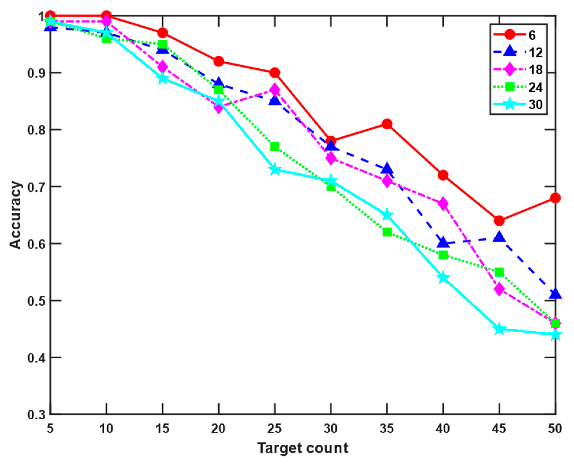
4.4. Impact of Sensor Quantity

In our algorithm, multi-sensor scenarios are defined not as two or three sensors, but as significantly larger quantities. This section investigates the impact of varying sensor counts on algorithmic performance. By increasing the number of sensors in scenario 1 from 6 to 30 in linearly spaced increments, we analyze the effects on both running time and association accuracy.

Figure 11 and Figure 12 demonstrate that increasing the number of sensors leads to increased running time and reduced algorithm accuracy. The increase in sensor quantity means that given the same number of targets, more track points are generated. This results in a larger dataset for real-time track association calculations, leading to correspondingly increased running time. When the number of targets is fewer than 10, an increase in sensor quantity may not necessarily lead to a decline in association accuracy, as shown in Figure 12. There are two main reasons for this. First, with a smaller number of targets and larger activity areas, the spacing between targets is sufficiently wide. Even with significant sensor measurement errors, the detected track points after clustering cannot be misassigned to other targets. Second, the tracks are randomly generated. When two randomly generated tracks overlap and intersect while having nearly identical headings and speeds, even the smallest measurement errors cannot prevent incorrect associations. When the number of targets exceeds 10, it becomes clearly visible that as the target count increases, the association accuracy declines. Moreover, the more sensors there are, the worse the algorithm performs.

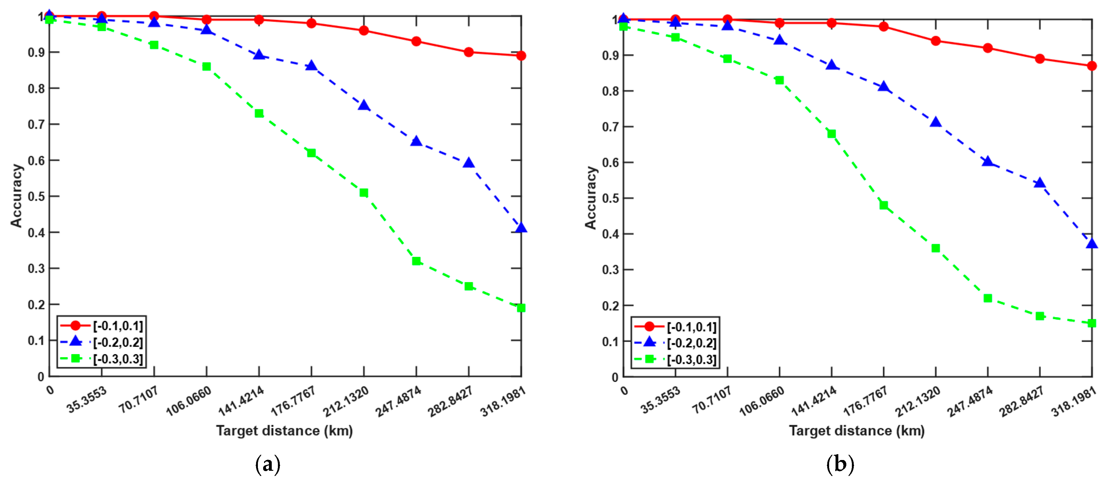
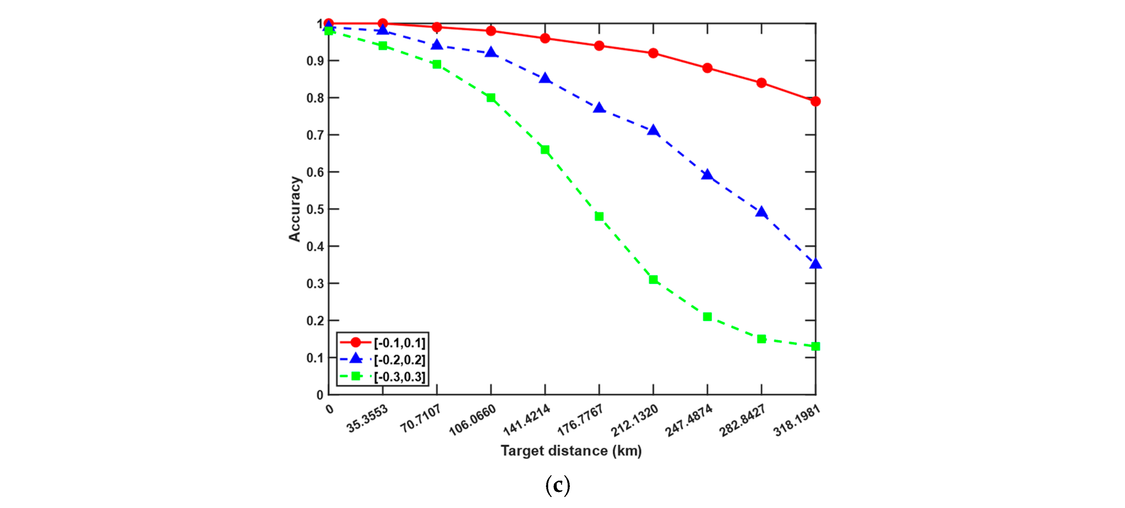
4.5. Impact of the Target Distance

As discussed above, the essence of the impact of target distance on track association lies in its amplification and attenuation of sensor errors due to changes in distance. It is intuitive that the farther the target distance, the greater the impact of the errors on the measurement, as shown in Figure 5. We define the distance from the center of the target activity area to the origin of the two-dimensional coordinate system as the target distance d_t and the area of the generated region remains constant. The range of d_t is from 0 to $250\sqrt{2}\approx 353.5534\hspace{0.33em}\mathrm{km}$, with values taken uniformly at $25\sqrt{2}\approx 35.3553\hspace{0.33em}\mathrm{km}$ intervals. In scenario 1, the original parameters are kept fixed except measurement errors, and we consider the association accuracy under different errors.

As shown in Figure 13, each subfigure shows the impact of different azimuth measurement errors and target distance on accuracy under the corresponding slant range measurement error, and the values of these errors are representative. It can be seen that when the target distance is greater, the measurement errors are amplified, and the decrease in accuracy is particularly noticeable. In long-range detection, the relationship between measurement errors and association accuracy becomes significantly weaker and may even exhibit nonlinear or inversely correlated trends due to geometric error amplification, target sparsity, and resolution limits. Therefore, for the algorithm proposed in this paper, the closer the overall activity area of the target is to the sensors, the better the detection performance, the smaller the spatial error, and the higher the association accuracy.

5. Conclusions

T2TA is a fundamental and critical issue in multi-sensor multi-target information fusion. Particularly in complex electromagnetic environments, achieving real-time, non-exhaustive track association for multi-target data originating from multiple sensors presents significant challenges.

This paper proposes a track association method based on the SAS-KNN-DPC algorithm, which enables real-time clustering in a non-exhaustive manner. By introducing a step-2 temporal neighborhood affinity matrix under a non-registration framework, the algorithm eliminates the need for temporal registration, significantly reducing error propagation while maintaining real-time performance. Multi-feature track-point fusion similarity integrating positional and kinematic data and its corresponding matrix are proposed, enhancing feature utilization efficiency. The self-adaptive step-2 truncation distance is also proposed to adjust to data distribution dynamically, improving robustness in dense and noisy environments. With the self-adaptive multi-feature similarity truncation matrix proposed, cluster centers are determined and assignment association is completed, achieving simultaneous clustering and real-time track association. Experimental results demonstrate that SAS-KNN-DPC outperforms existing methods in both association accuracy and computational efficiency, as discussed in the Experiments section.

In the next phase of research, we will focus on two main tasks. First, we will test and improve the algorithm using more extensive spatiotemporal track datasets. Second, building upon this research and inspired by stability-preserving strategies, we will develop new real-time online track association algorithms and put them into practice.