Abstract
This paper aims to describe a method of non-destructive testing in highly variable production using a robotic ultrasound diagnostic system. Highly variable production involves producing products of different shapes and dimensions, which requires flexible positioning and the adaptation of diagnostic technology. Typically, highly variable products are made in small batches. Implementing automation tools, including robotic systems, can meet this requirement, even in diagnostic processes that demonstrate the required quality level. This paper deals with the design, simulation, optimization, and verification of an innovative robotic ultrasound diagnostic system for non-destructive testing in highly variable production environments. The robotic positioning of the diagnosed object and the ultrasound probe achieves the automatic adaptation of the system. Robots can automatically position the ultrasound probe relative to the diagnosed object using laser distance measurements in the water environment of a diagnostic vessel. Computer processing of the data measured by the ultrasound probe enables the evaluation of data and the documentation of quality criterion fulfillment in digital form. Setting the technology parameters, monitoring the technology status, and displaying the quality control results are enabled by a human–machine interface system also described in this paper.
1. Introduction
In industrial production, an inefficiently tuned manufacturing process can induce wastage of material, energy, and human potential. In industrial practice, some tangible sources of feedback of such a manufacturing process are a low-quality product, excessive resource consumption, and a negative impact on human health.
A solution to this problem may be the implementation of innovative manufacturing technologies, which would enable workers to work under more comfortable conditions with minimal negative impacts on the workforce and the environment and, what is more, with the potential to increase the quality of the final product.
Kustroń et al. in [1] stated that the rapid growth of production seeks to increase product quality and minimize costs. To reach the required product quality, it is necessary to integrate quality control technologies into manufacturing systems. To make the quality control process effective from the standpoint of reducing expenses needed for performing quality control, it is reasonable, in connection with the manufacturing process, to implement automated quality control workplaces using robots controlled by central control systems with a high degree of intelligence. Such diagnostic systems intended for automated quality control will allow effective adaptation to variable products during final quality inspection or when testing semi-finished products in the production flow. The capability of the workplaces to automatically cope with the variability of manufacturing and control processes makes such workplaces desirable for quality control that can also be used in changing and highly variable manufacturing in small- and medium-sized enterprises.
Lofving et al. stated in [2] that flexible automation in production operations brings with it a great potential to increase the competitiveness of the ability of manufacturers of small production series, where it has traditionally been problematic to automate processes of highly variable and small batches of varying demands.
Highly variable and small-batch production is typical for small- and medium-sized enterprises, where the implementation of robotic workplaces provided with cybernetic systems is crucial to enabling flexible adaptation while reducing human interventions to a minimum.
The authors noted in [3] that relatively low flexibility is one of the main disadvantages of mass production technologies. Relative inflexibility is also characteristic of diagnostic workplaces in mass production factories.
Regarding cost minimization and economic efficiency, it is inappropriate for small- and medium-sized enterprises to use robotic workplaces designed for mass production. In such enterprises, implementing digital tools and robotic systems with a strong ability for automatic adaptation is necessary to increase production efficiency. Before implementing these flexible manufacturing systems, validating designs in a virtual environment is practical using data modeling and simulation tools. To achieve the variability of robotic workplaces, it is reasonable to use robots whose control systems can coordinate in a robot team so that they can handle, process, and diagnose products of different sizes and shapes, since the product range in small- and medium-sized enterprises is highly variable.
For example, in the automotive industry, workpieces are clamped in fixed jigs, as described by Halim et al. [4]. By using fixed jigs, it is impossible to change the workpiece positions flexibly and automatically. The positioning of the variable parts is thus limited by the prepared position of the jigs, which are designed to hold a specific type of part.
Robot and gripping technologies are relatively flexible components of production technology. On the contrary, jigs have the lowest degree of flexibility. The type and number of holding elements and clamps as well as the number of parts and the required procedure for connecting them are typical for a jig, the parameters of which are determined for its specific type, as mentioned by Kampker et al. in [5].
Predetermined positions must be secured in the pre-preparation phase before the production process, which again reduces its efficiency and economic return.
Although there are flexible jigs, where a specific change is possible when in use, the flexibility of their use in production workplaces is not sufficient, due to the need for a relatively long time for their adjustment, as reminded by authors in [4].
An effective way to achieve flexibility in object positioning during both manufacturing and control operations is to replace inflexible solutions using flexible jigs by robotic positioning throughout the concerned operation. As far as control operations are concerned, in the case of flexible control systems implemented in industrial production, it makes sense to implement, in particular, non-destructive testing technologies. One of the well-known non-destructive testing methods of quality control is ultrasonic testing.
Ensminger and Stulen [6] mentioned that devices for ultrasonic non-destructive testing have come a long way since their inception in the 1940s, being applied to the most advanced systems. This highly sophisticated diagnostic ultrasound system development was also possible thanks to computer technology and progress in analog–digital electronics. Computer plug-in cards are used to integrate ultrasound diagnostic systems. The components of these plug-in cards are a pulser, receiver, analog-to-digital converter, and digital signal processing. With these commercially available devices, building highly efficient ultrasonic testing applications is possible while meeting specific requirements.
Ultrasonic NDT inspection is of great importance when searching for defects in tested objects in an industrial environment, as it is, together with other advanced scanning methods, a reliable diagnostic method suitable for repetitive control processes, as stated in [7] by Madhumitha et al.
Kustroń et al. stated in [1] that the usability of the component in different production phases, even after quality control, the repeatability of the method, and high repeatability and efficiency are the main advantages of the non-destructive testing of structures using the ultrasound diagnostic method. Compared to other non-destructive testing methods (e.g., radiographic, magnetic particle, liquid penetrant), the ultrasound method offers the advantage of eliminating the need for operator-protective measures and minimizing the impact of the application of this method on the environment.
Figure 1 from Kustroń et al. [1] shows the laboratory test station that allows the positioning of the ultrasound probe relative to the weld. The solution shown in Figure 1 is characterized by an insufficiently variable system of positioning in liquid, both of the ultrasound probe and the scanned object. The robotic positioning of the ultrasound probe by the industrial robotic manipulator described in this paper provides a high degree of variability of ultrasound probe positioning, even in liquid, as described in the following sections of this paper.
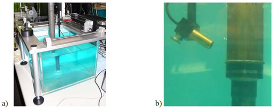
Figure 1.
The ultrasound scanner (a) and the orientation of the transmitter to the weld (b) [1].
The variability of robotic workplaces in placing products in the position required to perform the joining, machining, or diagnostic process can be achieved by the robotic placing or robotic holding of the object during the entire process. As stated in this paper, in the robotic ultrasound diagnostic system for non-destructive testing in highly variable production, a robotic manipulator is used for positioning during the diagnostic process and, in the case of cylindrical objects, the seventh axis of the ultrasound diagnostic robot is also used. In the preparatory phase, the robotic manipulator positions the diagnosed object in air or liquid. During the robotic diagnostic process, however, the analyzed object is positioned by the robot exclusively in a liquid that provides an environment suitable for the propagation of ultrasonic waves.
For the automated evaluation of a defect by a robotic ultrasound method inclusive of defining the defect positions, it is important to precisely bring in line the position of the diagnosed object in relation to the robotically positioned ultrasound probe.
According to the definition [8], the accuracy of a manipulator is a measure of how close the manipulator can come to a given point within its workspace. Repeatability measures how close a manipulator can return to a previously taught point. To determine the position and orientation of the end effector, there is typically no direct measurement of the robot. The position of the end effector is usually determined by indirect measurement using position encoders located on the motor shafts or the joints. The data measured in this way allow the final position of the effector to be derived. At the same time, in the calculations, we consider the manipulator’s geometry and rigidity. However, the actual position of the effector is also affected by quantities that are not included in the calculation of the position using the indirect method. Specifically, it concerns inaccuracies in calculations, machining accuracy, the backlash in gear bodies, the influence of the weight of the kinematic structure, and others. The manipulators are, therefore, constructed with extremely high rigidity to achieve the required accuracy. Otherwise, the accuracy of the positioning of the end effector could be achieved, for example, by using a vision system for direct measurement of the end position of the effector.
By grouping multiple robotic manipulators designed to perform one common task in a shared workspace, the accuracy of the required process is affected by the accuracy of all individual robotic manipulators that make up the robot team. The accuracy of each member of the robotic team (consisting of robotic positioners and the ultrasound diagnostic robot) affects the mutual position of the object and the ultrasound probe during the diagnostic process.
Computer vision makes the precise positioning of robotically held diagnostic parts and ultrasound probes possible, resulting in the acquisition of a big data cloud describing the scanned space. In vision-based robotic positioning, the selection of a robust and relevant set of measurement data needs to be addressed, as described by Spong et al. [8]. In [9], Bologna et al. stated that computer vision in multi-transition applications runs into limits due to high variability in slot depth, illumination conditions, and blind spots, which, at the same time, leads to a decrease in image processing performance.
Using a set of laser distance sensors that scan the area of interest from different angles eliminates this problem, as described in the present paper. Laser distance scanners are used in the robotic ultrasound diagnostic system for non-destructive testing in highly variable production for the robot’s automatic positioning of the ultrasound probe. The suitability of the use of feedback control of the position of the robotically positioned ultrasound probe concerning the diagnosed object was demonstrated by the verification test described in this paper.
The interconnection of mechatronic systems, such as industrial robots, sensing systems, and digital tools, enables automatic diagnostics to be carried out with minimal need for human labor, even in the environment of small-batch highly variable production, as described by authors in [10]. Figure 2 shows an example of a design of such an autonomous diagnostic workplace using robots.
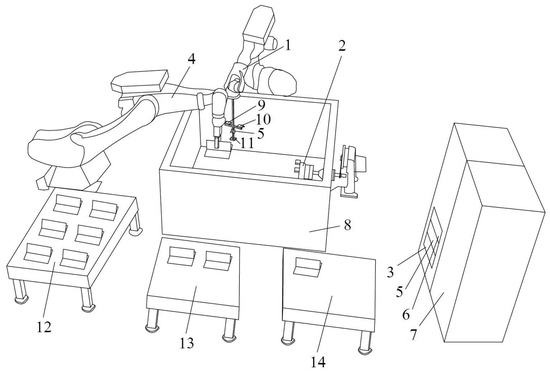
Figure 2.
A layout of the system of intelligent robotic ultrasound diagnostics [10]. 1—diagnostic robot, 2—rotational external axis of the robotic system, 3—system of the automated robotic positioning of the ultrasound probe, 4—robot for manipulating a diagnosed object, 5—manipulation robot control system, 6—data processing computer and database, 7—control system of the workplace, 8—vessel, 9—laser scanner No.1, 10—laser scanner No.2, 11—laser scanner No.3, 12—warehouse of the to-be-diagnosed objects, 13—warehouse of the quality OK objects, 14—warehouse of the quality NOK objects.
Liu et al. [11] described that rapidly developing computer technologies enable the direction of the manufacturing industry toward intelligent production. The effective adaptation of production technologies to changing product requirements requires the minimization of warehouse stocks, and ubiquitous connections can be achieved by implementing smart solutions. Industry 4.0 brings space for the research and development of applications that connect the cyber and physical world of production technologies intending to build smartly embedded and networked systems. A means for innovative production technologies is also the digital twin, which enables the creation of a tool for the simulation, monitoring, optimization, and management of production technologies through data and models of technological equipment and algorithms. With this tool, it is also possible to process data obtained in real-time from digitally controlled and monitored production technology.
Ferro et al. [12] state that the digital twin, as the counterpart of a technological unit, first appeared in the aviation industry. It has recently been transferred to the manufacturing sector, where it is gradually finding applications for process simulation. In addition to pure data, the digital twin also contains algorithms and can make production decisions. A digital twin verified the design of the robotic ultrasound diagnostic system for non-destructive testing in highly variable production, as described in this paper.
The digital communication link between the robots and the quality evaluation software allows the regrouping of objects at the workplace exit into sets—high-quality and low-quality products. Thus, it automatically controls the flow of products within the production process.
As Dumic et al. described in [13], the availability of RGB-D cameras and 3D scanners provides the possibility of their practical use in industrial production. The problem is not the image capture but the interpretation of information from a large cloud by measuring the obtained data from the end user, who is often a human.
The cloud of data obtained from robotic ultrasound diagnostics described in this paper is presented in a 3D image with color highlighting of the defects identified by the ultrasound method, as shown in Section 8. This 3D view synthesizes and visualizes data defining the position of robotically positioned objects with data obtained by ultrasonic measurements.
The present paper describes the design, simulation, verification, and validation of the robotic ultrasound diagnostic system for non-destructive testing in highly variable production. This system has the potential to increase the level of automation for inter-operational and final inspection processes by using a non-destructive method of robotized testing in industrial production conducted in line with the concept of Industry 4.0.
The robotic ultrasound diagnostic system’s novelty for non-destructive testing in highly variable production is the automatic computed numerical control of the ultrasound probe’s robotic positioning in the diagnostic tank’s liquid environment.
Automatic robotic positioning is controlled based on feedback from three laser distance sensors located in the triangle’s vertices. The robot’s ultrasonic probe is placed inside the space around these sensors.
Simultaneous synchronous robotic positioning of the diagnosed object with the robotically positioned ultrasound probe is also innovative. Thanks to the robotic positioning of the probe and the workpiece, the prototype of the robotic ultrasound diagnostic system for non-destructive testing can diagnose products of various sizes and shapes. This system predetermines the workplace for use in small-series, highly variable production typical of small- and medium-sized enterprises.
The connection of the robotic system with the central database of products makes it possible to archive data from the processes of the automated quality control of products by unique identifiers and to assign defect types to them. This fact predetermines a robotic workplace for the generation of data on the quality of products, which will be used in conjunction with the production database to train new neural networks aimed at classifying defects and optimizing production processes in modern industry.
Data pre-processing and their fusion are automatically implemented in the environment of an innovative application, which is part of the diagnostic robotic workplace and enables comfortable 3D views of the diagnosed objects, including their internal defects.
2. Design of Robotic Ultrasound Diagnostic System
This paper aims to describe the design of a robotic ultrasound diagnostic system for small-batch, highly variable production. When designing and implementing, the requirement is to maximize the degree of automation both in production mode and when switching to new-type object diagnostics.
The robotic ultrasound diagnostic system includes a robotic manipulator (1) for positioning diagnosed objects of various types. Grasping objects of multiple types is possible using a robotic gripper quick-change system (2). Automated robotic grasping by the corresponding robotic gripper is coordinated by a control system (3). The robotic manipulator transfers objects from the to-be-diagnosed object warehouse (4) into the liquid environment of the diagnostic vessel (5). The ultrasound probe (6) is positioned during the diagnostic process by an ultrasound diagnostic robot (7). Part of the robotic ultrasound diagnostic system is an external rotation axis (8).
Inside a diagnostic vessel (5) is a diagnostic table (9) on which a diagnosed object can be placed robotically, and then the diagnostic process can be carried out. After completion of the diagnostic process, based on the results of quality control by a non-destructive ultrasonic method, the objects are robotically positioned either in a quality object warehouse (10) or a low-quality object warehouse (11). The robotic ultrasound diagnostic system is designed to check the quality of objects of different shapes and sizes. For this reason, the diagnostic vessel (5) is equipped with liquid level measurement (12) intended to maintain the required liquid level height in the diagnostic vessel with the help of the control system (3). The liquid for maintaining the necessary level height in the diagnostic vessel (5) is stored in an auxiliary vessel (13) connected with the diagnostic vessel (5) by a pipe provided with a pump (14) and a filter system (15) to maintain the necessary purity of the liquid in which the objects are diagnosed. Entering the requirements of the robotic ultrasound diagnostic system by an operator and displaying the measured values from the ultrasound diagnostics are possible through an HMI system (16) on the computer screen. The execution of proper robotic ultrasound diagnostics is coordinated by the central control system (3). The robotic manipulator and the ultrasound diagnostic robot cooperate in the area covered by a safety system (17). The design of the robotic ultrasound diagnostic system is shown in Figure 3.
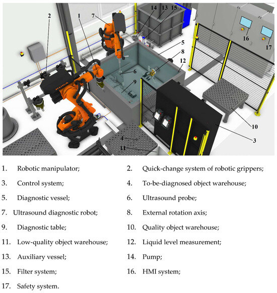
Figure 3.
Parts of the robotic ultrasound diagnostic system.
The effector of the ultrasound diagnostic robot was designed to enable the diagnostic robot’s automatic adaptation to the object’s curved surface. For this reason, the effector is equipped with three laser distance sensors (1, 2, 3) which provide feedback for the automated generation of the diagnostic robot trajectory. An ultrasound diagnostic probe (4) is placed in the tool center point of the effector, which diagnoses the object’s internal space in the analyzed object’s determined elemental volume. The laser distance sensors and the probe are installed on a holder (5) that ensures their sufficient separation from the flange of the industrial diagnostic robot so that the robot flange (6) does not sink into the liquid even in the case of diagnosing larger objects. A detailed look at the robotic ultrasonic effector is shown in Figure 4.
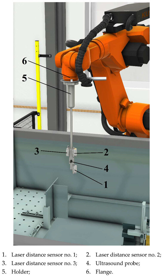
Figure 4.
A detailed look at the robotic ultrasonic effector.
3. Simulation of Robotic Ultrasound Diagnostic System
The design of the robotic ultrasound diagnostic system was verified in the Kuka.SimPro V3.1.1 simulation tool. The robots were placed in a 3D virtual environment relative to the coordinate system of the whole. The robots were assigned respective effectors with designated tool center points. The effectors were modeled in 3D CAD software CREO Parametric V7.0.3.0 and, together with the parameters, transferred to the simulation tool.
Similarly, the static parts of the workplace, such as containers, switchboard cabinets, robot control system cabinets, security systems, warehouses, etc., were imported from 3D CAD into the simulation tool. Signs were defined for the robotic manipulator, ultrasound diagnostic robot, and external rotation axis. The signals connected the robots and the positioner so their activities could be mutually coordinated. Subsequently, motion sequences were simulated for different diagnosed objects (see Figure 5).
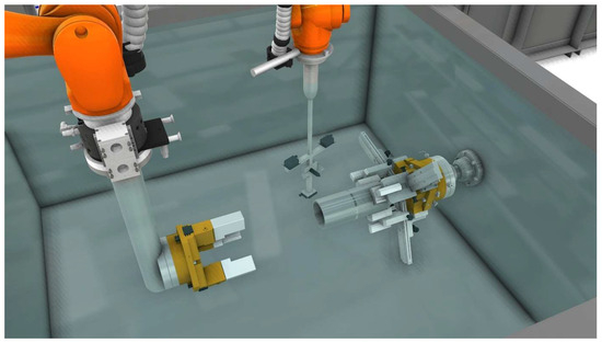
Figure 5.
The robotic ultrasound diagnostic system, including the communication connections of its components in a simulation tool.
Robotic grippers for grasping various objects are stored in a quick-change system of robotic grippers. First, the robot automatically grasps a robotic gripper for inserting cylindrical objects into the diagnostic vessel. Then, the robot grabs the object from the to-be-diagnosed object warehouse. Video from the simulation shows the robotic positioning of a cylindrical object into the vessel. During the diagnostic process, the cylindrical object is rotated using the horizontal 7th axis of the robotic system.
In contrast, the industrial robot (the 1st to 6th axes of the robotic system) positions the ultrasound probe. After completing the process of robotic ultrasound diagnostics, the object is picked out from the diagnostic vessel. The video at https://youtu.be/6HiUdjBfSRM?si=Ps0BgA9qumisAZme accessed on 14 May 2025 shows a robotic ultrasound simulation of cylindrical object diagnostics using simulation software.
KUKA.SimPro V3.1.1 was used to verify collision-free operation, joint-axis limit adherence, payload handling, offline programming optimization, and sensor–probe integration prior to hardware commissioning. Five representative scan trajectories were simulated without any collisions, with estimated cycle times of 45 ± 0.5 s per complete scan path. All I/O signals for the robot–probe interface passed validation, and the laser sensor reach was confirmed across the workspace. Joint-axis limits and payload capacities were also tested to ensure compliance. A representative simulation is shown in Figure 5. A detailed quantitative comparison of the simulated versus real-world performance was beyond the scope of this study and will be pursued in future work.
4. Method for Automatic Robotic Positioning of Ultrasound Probe
Automatic positioning of the ultrasound probe is realized using a six-axis industrial robot when the ultrasound probe is inserted in the tool center point of this robot. The robot is automatically positioned based on the feedback from three-point laser distance sensors measuring the distances from the plane of the surface of the diagnosed material in the vertices of the triangle, the inner surface of which also includes the area of intersection of the cone of the exciting signal from the ultrasonic wave with this plane. Feedback positioning based on laser measurement of distance was chosen to test diagnosed objects of variable shapes and sizes when the robot moves in different directions.
The configuration and number of point laser distance sensors were chosen due to the need to position the ultrasound probe relative to the object. To position the ultrasound probe to the object, it needs to be positioned in the following directions:
- Rotation of the probe around the vertical (Z) axis of rotation of the tool—information about the distance from laser distance sensors 2 and 3;
- Rotation of the probe around the horizontal (Y) axis of rotation of the tool—information about the distance from laser distance sensors 1 and 2;
- Bring the ultrasound probe closer to the desired distance from the object, using information about the distance from the laser distance sensors.
Before positioning the probe, it must be brought closer to the object at the distance at which laser distance sensors work. All laser distance sensors must point at the object. The system then automatically aligns the probe to the object. The ultrasound probe, laser distance sensors, and the robot share the same positioning coordinate system. The location of the laser point sensors on the effector is shown in Figure 6.
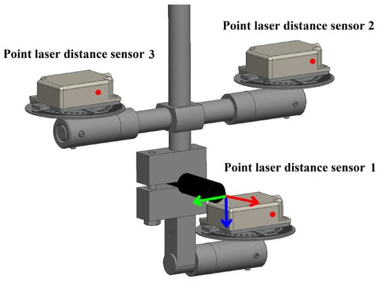
Figure 6.
Placement of the ultrasound probe and three laser distance sensors on the robotic effector.
The red dots in Figure 6 show the sources of the laser beams. The robotic diagnostic tool center point is shown as the origin of the coordinate system XYZ, where the red line means coordinate X, and the green line means coordinate Y. The blue line means coordinate Z. The distances between the sensors and the probe are shown in Table 1.

Table 1.
Absolute distances between the lasers and the probe in the Y and Z axes of the tool.
Length |dy| is the distance between objects, listed in Table 1, on the Y-axis of the coordinate system of the robot tool. Length |dz| is the distance between objects, listed in Table 1, on the Z-axis of the coordinate system of the robot tool.
To achieve automatic robotic positioning of the ultrasound probe based on feedback from three-point laser distance sensors, the program for generating the robotic trajectory must calculate the ultrasound probe’s actual real distance from the surface of the diagnosed object.
To concentrate measurement points as close as possible to the axis of the ultrasound probe, the calculation needs to include rotation angles of distance meters. The rotation of the distance meters about the vertical axis is shown in Figure 7. Distance meters D2 and D3 are rotated through an identical angle β. It is necessary to calculate the rotation angle αv that the ultrasound probe needs to be rotated through to be perpendicular to the plane. The angle for rotation about the vertical axis (rotation around a Z-axis that is in a home position identical to the axis perpendicular to the Earth’s surface) αv is calculated according to Formula (1):
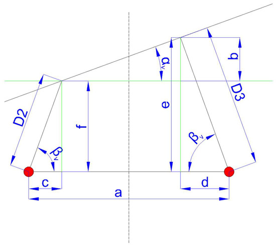
Figure 7.
Rotation of distance meters D2 and D3 about vertical axis.
The rotation of the distance meters about the horizontal axis is shown in Figure 8. Distance meters D1 and D2 are rotated through an identical angle γ. The angle for rotation about the horizontal axis (Y-axis of the coordinate system with the origin in the robotic tool) αh is calculated according to Formula (2):
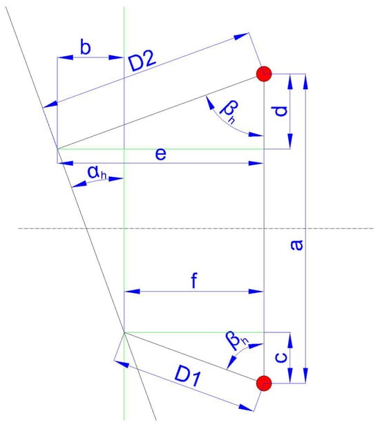
Figure 8.
Rotation of D1 and D2 laser distance meter about horizontal axis.
The automatic robotic positioning of the ultrasonic probe, based on feedback from three laser sensors, was first tested in the air environment. Subsequently, the automatic robotic positioning of the ultrasound probe was tested in liquid, as shown in Figure 9.
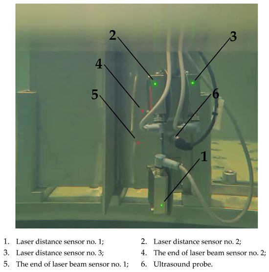
Figure 9.
Testing the robotic positioning of the probe in the liquid based on laser distance measurement.
Before positioning the probe in the liquid environment, the distance sensors needed to be calibrated, as they measured values in the diagnostic liquid differently from those in the air environment.
For the calibration of distance measurement using a laser distance sensor (LDS) in an aquatic environment, an experiment was conducted to determine the relationship between the real distance and the distance measured by the laser sensor. Figure 10 shows how this experiment was conducted. The laser rangefinder was fixed at a static distance from the bottom of the water-filled tank. The laser beam, type optoNCDT ILD1402-200.013 MICRO-EPSILON, Ortenburg, Germany, with a linearity deviation less than or equal to 0.18% FSO, was directed perpendicularly to the tank’s bottom. The distance between the laser rangefinder and the tank’s bottom was 254 mm, and the distance measured by the laser scanner was 195.3 mm (first row of Table 2). In further measurements, calibrated plates of known thickness (shown in Figure 10) were inserted into the path of the laser beam at the bottom of the tank. This allowed us to precisely determine the thickness by which the distance between the laser rangefinder and the measured point on the surface of the plate was shortened.
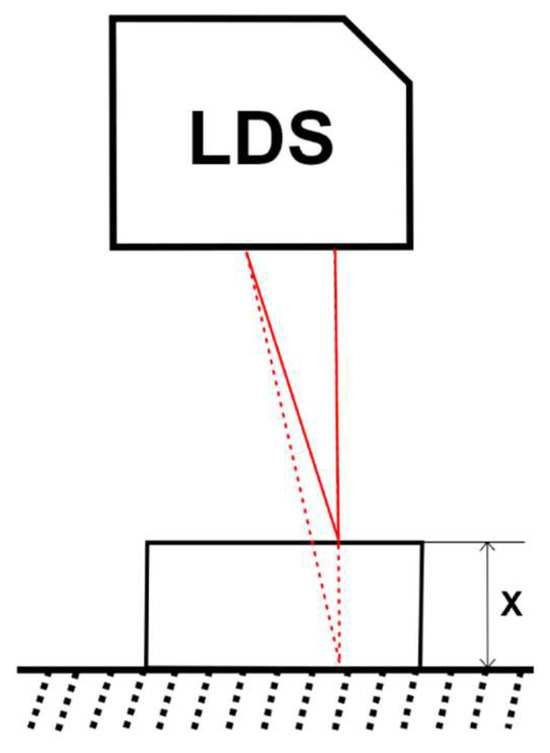
Figure 10.
Laser scanner distance measurement experiment to determine correction function.
Table 2.
A data table of the distance measured by a laser scanner and the distance measured by an etalon.
From the data (Table 2) measured during the calibration of the sensors for use in a liquid environment, the necessary transfer characteristic (Figure 11) of the laser distance sensor was determined, as was the dependence for calculating the distance value between the surface of the object and the robot’s effector in the liquid.
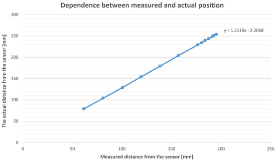
Figure 11.
A chart of the transmission characteristics between the laser-sensor-measured distance and the etalon-measured distance.
Based on the measured data and the dimensions of the calibration plates, the measurement errors were determined as the difference in values based on the measured values of the calculated length and the known calibrated thickness of the leaves. The results of these measurements and the calculated errors obtained thanks to verification measurements are shown in Table 3.
Table 3.
Measured values of the calculated length, the known calibrated thickness of the leaves, and measurement errors.
The experiment demonstrated that applying a correction transmission characteristic to a set of data measured by the scanner makes it possible to successfully use a laser scanner originally calibrated for distance measurement in air and also for distance measurement in the liquid environment of the diagnostic tank. During the testing of the laser rangefinder, the effect of temperature, liquid flow, and the presence of foreign bodies in the liquid was simulated by blowing in the air, which caused the formation of bubbles in the liquid. Experiments have shown that liquid flow and temperature do not fundamentally influence the accuracy of the measurement and its subsequent reliability in the feedback control of the position of the diagnostic robot. However, the bubbles had a significant effect, making measuring the distance impossible. The presence of foreign parts negatively affects the quality of measuring the distance of the robotic effector from the surface of the diagnosed object. In this case, it would be impossible to control the diagnostic robot’s position based on laser rangefinders’ feedback. For this reason, the prototype of the workplace of robotic ultrasound diagnostics was equipped with water management, which includes a filter system for eliminating the influence of foreign bodies on robotic ultrasound measurement that brings reliability.
5. Robotic Positioning of Diagnosed Objects in Liquid Environment
When diagnosing the quality of products of variable dimensions and shapes, the robotic ultrasound diagnostic system for non-destructive testing must be able to handle various objects by a robot automatically. For this purpose, the robotic manipulation of objects of different shapes and sizes was proposed, verified by simulation, and validated in a robotic ultrasound diagnostic system prototype. The tested prototype of the robotic system offers several options for the robotic picking of objects from and their placement in warehouses, as well as the robotic holding of the diagnosed object during ultrasound diagnostics. The first option shown in Figure 12 is placing the object in the diagnostic position and holding it by a six-axis industrial robot during the diagnostic process. This option offers robotic manipulation of the object in the liquid environment of the vessel during ultrasound diagnostics performed by the ultrasound diagnostic robot. The advantage of this option consists of the ability of robotic manipulators to position the object and the probe in such a way as to cooperate to enable the diagnostics of highly variable products. However, this type of positioning is slower than the following two options suitable for less variable products (pipe or plate). Figure 12 shows, on the left, the testing of the robot’s cooperation by diagnosing a filet weld object and, on the right, the robotic ultrasound diagnostic process of a butt weld.
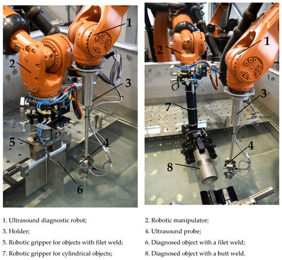
Figure 12.
Locating into a diagnostic position and holding the diagnosed object during the diagnostic process by a 6-axis industrial robot: left: diagnostics of a filet weld; right: diagnostics of a buttweld.
In the second option (Figure 13), the robot puts a diagnosed object on the diagnostic table inside the diagnostic vessel. Fixtures installed on the table in the diagnostic vessel stabilize the object. The advantage of this solution consists of streamlining the diagnostic process for frequently repeated objects of a known shape, life extension of the positioning robot, and the reduction in computational complexity, as there is no need to coordinate the simultaneous positioning of two robotic manipulators. In Figure 13, on the left, the positioning of the ultrasound diagnostic robot around the diagnosed object during the diagnostic process is shown. In Figure 13, on the right, details of the stabilization fixtures can be seen.
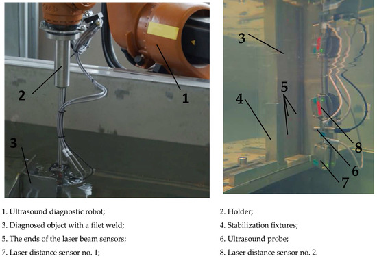
Figure 13.
Diagnosed object placed on the diagnostic table inside the diagnostic vessel in the course of the diagnostic process: left: ultrasound diagnostic robot; right: a detail look at the stabilization fixtures.
In the third option (Figure 14), the robot places the object into the vessel and puts it into the gripper of the external axis. During the diagnostic process, the object rotates about the seventh (external) rotation axis. This option is suitable for positioning cylindrical objects whose diameter corresponds to the grasping capabilities of the robotic rotary gripper on the seventh axis of the ultrasound diagnostic robot. In this case, it is necessary to coordinate the positioning of the seventh axis with the ultrasound diagnostic robot, which is realized through the robot’s control system.
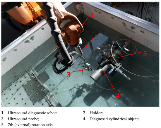
Figure 14.
An object rotating about the 7th (external) rotation axis during ultrasound diagnostics.
6. Description of Robotic Diagnostic System Experiments
In this part, we focused on testing and detecting the accuracy of the robotic workstation, designed for ultrasonic diagnostics of materials to detect potential defects. Our main platform is a Fanuc CRX-25iA collaborative robot that manipulates an ultrasonic probe (Figure 15). The measurements were performed in a water-filled tank where the test objects were placed (Figure 16). The control measurements we performed were carried out on the scale defined by ISO7963 (Figure 17), which provides accurately defined reference values for assessing the accuracy and reliability of the diagnostic system. Figure 17 shows the reference values of the measured quantities.
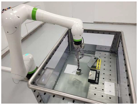
Figure 15.
Workplace of robotic ultrasound diagnostic system for non-destructive testing.
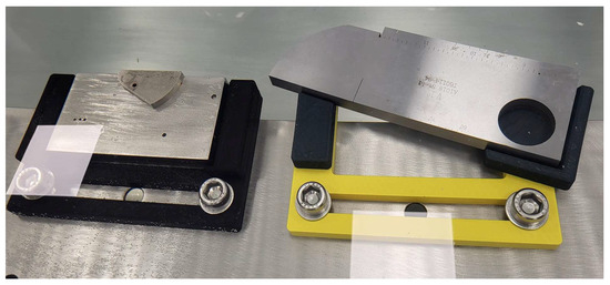
Figure 16.
Location of objects.
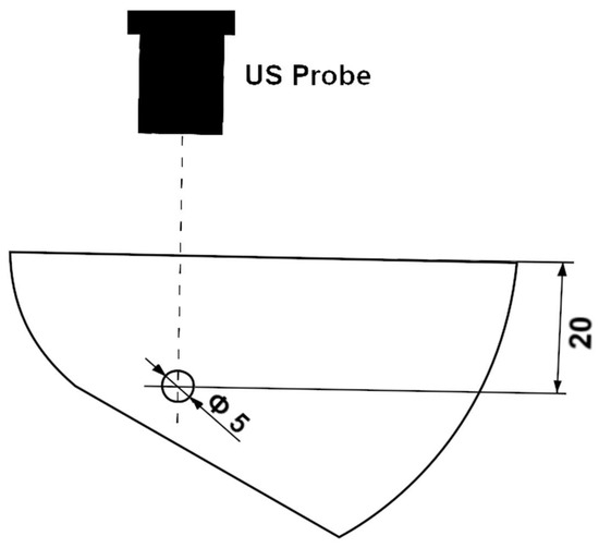
Figure 17.
Important dimensions from ISO7963.
In our study, we investigated in detail the accuracy of the robotic workstation through three different types of measurements:
- Static measurement;
- Static measurement from a random position;
- Dynamic measurement.
The first types of measurements were static measurements at a single point (Figure 17). These measurements were performed to obtain accurate data on the accuracy of the workstation under steady and unchanging conditions. The robotic system was placed at a designated point. Then, we analyzed how accurately and stably it could measure the distance of the input echo, the error echo, and their distance, determining the depth at which the defect is located.
The second type followed the same parameters. Measurements were also taken at a single point (Figure 17), but the robot arrived at the same point from a randomly generated position. This simulated real working conditions, where it is essential that the robot maintains accuracy even under variable positions. Such measurements show how the robotic manipulator’s precision and repeatability affect the measured quantities’ accuracy.
The last type of measurement consisted of testing the measurement in motion. The robot moved the ultrasound probe in front of the defect (Figure 18). Here, we observed how well we could determine the size of the defect and the depth at which it was located. In doing so, we observed how the speed of movement affects the accuracy of the measurement.
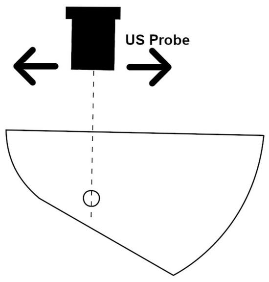
Figure 18.
Dynamic measurement.
These three measurements give us a comprehensive view of the capabilities and accuracy of our robotic ultrasound diagnostic workstation.
6.1. Static Measurement
This measurement aimed to determine and analyze the accuracy of the measurement and quantify the noise in the static measurement. As the figure indicates (Figure 17), the ultrasonic probe was robotically positioned directly in front of the hole at a standard scale. This hole has a diameter of 5 mm, and its center is 20 mm from the edge of the scale bar. This means that the distance between the input echo and the defect echo should be 17.5 mm, as it will show up on the ultrasound diagnostics when the ultrasound wave passes from one type of material to another. The resolution of the diagnostic software depends on the setting of the measurement range, i.e., the depth the user wants to analyze. In this case, the range was set to 50 mm, and the distance resolution reached a value of 0.1037 mm. The following graph (Figure 19) shows the signal waveform of one “A-scan” measurement with the blue line. The calculated real distance from the ultrasound probe is on the X-axis, and the received echo intensity is on the Y-axis. The first wider echo on the graph corresponds to the transition of the sound wave from the water to the scale. The second narrower echo corresponds to the transition of sound waves from the scale to the water in the hole. If the echo is saturated, the position of the first signal value above 95% is considered. An example of such an echo is the first input echo. Thus, the distance between the first and second echoes determines the depth at which the defect is located.
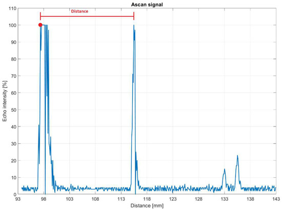
Figure 19.
A-scan-received echo signal.
Echo intensity in an ultrasound resectoscope measures the strength of the reflected ultrasonic wave as a percentage of the initial transmitted wave. Although it is commonly represented in decibels (dB), we have presented it as a percentage in Figure 19 for ease of interpretation.
The following formula defines the echo intensity (%) shown in Figure 19:
where is the amplitude of the reflected echo, and is the amplitude of the initially transmitted wave. This conversion provides a straightforward way to understand the relative strength of echoes.
Regarding the attenuation of ultrasonic waves and the significant difference in acoustic impedance between water and the object being inspected, ultrasonic waves indeed attenuate as they propagate through a medium due to absorption and scattering effects, leading to a decrease in wave amplitude. The notable observation that the second echo still reaches 100% intensity is attributed to the wave saturation. The input echo is saturated and wider than the returned echo, indicating that the initial pulse has a higher energy density, resulting in a wider signal. The second echo, while still reaching 100% intensity, appears thinner due to the reduction in energy density as the wave travels and interacts with the material structure. The 100% intensity for the second echo indicates that it is normalized to reach 100% and the intensity of the first echo is clipped to 100%. Its higher intensity is evidenced by the width of the input echo and its saturation.
The following graph (Figure 20) shows the results of the static measurement. A total of 2000 measurements were taken without moving the robot. The first plot shows the position of the input echo for each measurement. The second graph shows the position of the echo caused by the hole in the scale. The third graph shows the calculated distance between the echoes. This distance expresses the depth at which the defect is located. We can see that the measurement noise is minimal at a given resolution. The standard deviation of the depth at which the defect is located is 0.0338 mm. The average deviation from the reference value of 17.5 mm is 0.0088 mm. However, this is a static measurement, and these results tell us that the ultrasound diagnosis produces quite stable results. In further experiments, the movement of the manipulator will already enter into the measurement results.
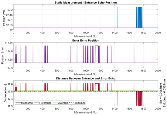
Figure 20.
Entrance and error echo positions and the distance between them for static measurement.
6.2. Static Measurement from Random Position
The following test shows the effect of the accuracy and repeatability of the robotic manipulator on the measurements made by the proposed system. The experiment involved 500 repetitive cycles, each consisting of several steps, to assess how well the system handles randomly generated start positions and maintains the accuracy of the measurements. In each cycle, the robot was given randomly generated XYZ coordinates, and only the R angle for the tool center point (TCP) was randomly generated from the orientation defined by the WPR angles for safety. These coordinates were randomly selected from the tank space to ensure the collision-free movement of the robot. The robot then performed a collision-free motion to a randomly selected position and returned to the predefined measurement position when this position was reached. After returning to the measurement position, the robot waited 1 s to ensure the motion was completely stopped and the system stabilized. After this waiting time, the measurement started and lasted 5 s. In this way, we obtained sufficient data to assess the accuracy and reliability of the measurements. This whole process was repeated 500 times. The average scanning frequency reached a value of 11.2 Hz. This means that an average of 56 A-scans were measured in each cycle. Thus, a total of 28,000 A-scans were measured. The results of this experiment can be seen in the following graphs. The first graph (Figure 21) shows all the measured raw data. It can be seen that the average value of the distance of the defect from the surface of the material was close to the reference value (17.5 mm), and the average deviation reached 0.0035 mm. The standard deviation increased as expected and reached a value of 0.0685 mm. The results of the average filter included in the evaluation are shown in the same figure. In each measurement cycle, the measured values were averaged. The graph shows the results of the filtered measurements from 500 measurement cycles. The mean deviation did not change, but the standard deviation converged almost to the value of the static measurement and reached a value of 0.0398 mm. These results show that the measurements should be repeated at one point for the best results, and an average filter should be included in evaluating the A-scans.
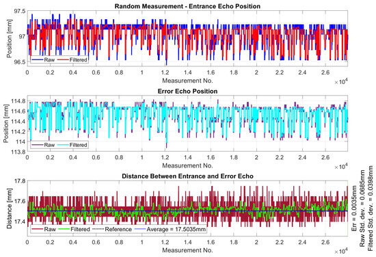
Figure 21.
Entrance and error echo positions and the distance between them for measurement from random robot starting positions.
6.3. Dynamic Measurement
During the dynamic measurement, the ultrasonic probe was moved in front of the material to obtain detailed information about the width of the defect and the depth at which it is located. Experiments involved moving the probe progressively before the material surface and monitoring the echo signals produced as the probe passed through the defect region. These measurements were also carried out at the scale defined by ISO7963. During the experiment, the robot performed 250 measurement cycles. In each cycle, the robot traversed a linear trajectory 12 mm long such that the center of the defect was located at the center of the trajectory. Within a cycle, the robot traversed this trajectory in both directions, back and forth. The defect’s width was determined by finding the A-scan where it first appeared and last appeared in one pass. Based on the positions at the first and last A-scan, the defect’s width was calculated as the ultrasonic probe reached an average measurement frequency of approximately 11 Hz, indicating that the speed of the ultrasonic probe movement would affect the accuracy of the defect width measurement. As it is a circular hole, the depth at which it is located depends on which part of the hole the measurement would be taken. The depth at which the defect was located was determined from the A-scans, where the lowest distance to the edge of the material was detected. The experiment conducted trials at five speeds: 20, 15, 10, 5, and 2 mm per second. The following graph (Figure 22) shows the results for 20 mm/s and 2 mm/s speeds.
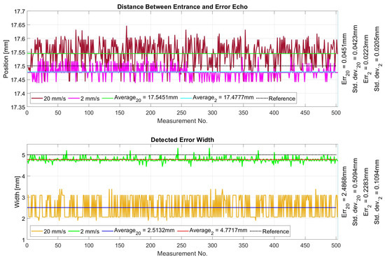
Figure 22.
Detected defect position and width results for measurements with 2 mm/s and 20 mm/s velocities.
The results show that the system’s accuracy depends inversely on the speed at which the robotic manipulator moves the ultrasonic probe. Thus, as the speed increased, the accuracy decreased. At a speed of 20 mm per second, the depth measurement achieved an average deviation of 0.0451 mm from the reference of 17.5 mm with a standard deviation of 0.0423 mm. At a speed of 2 mm per second, the mean deviation was 0.0223 mm, and the standard deviation was 0.0205 mm. When we look at the results of the defect width measurement, we see that at a speed of 20 mm/sec, the average width was determined to be 2.5132 mm, and the real diameter was 5 mm, so the deviation was 2.4868 mm from reality with a standard deviation of 0.5094 mm. At a speed of 2 mm/s, the defect width was determined to be 4.7717 mm, a deviation from the reference of 0.2283 mm, and a standard deviation of 0.1094 mm.
The following table summarizes the results of all measurements. Table 4 summarizes the measured data on the depth at which the defect is located and with what standard deviations the measurements were taken at the indicated speeds.
Table 4.
Measurement of defect depth below surface.
Table 5 shows the same for the defect width measurement.
Table 5.
Measurement of defect width below surface.
These results are displayed in graphs that show the absolute deviations of the measurements from the reference values as a function of the speed of motion, together with the associated standard deviations of the measurements. The graph in Figure 23 shows the increasing dependence of the measured depth at which the defect is located on the scanning speed. The standard deviation also increases with increasing speed. Figure 23 also shows an increasing dependence of the error of the measured defect width on increasing speed. Similar to the depth case, the standard deviation of the defect width measurement also grows with increasing speed.
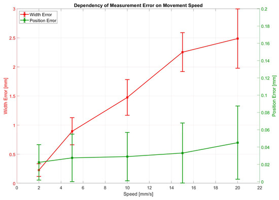
Figure 23.
Errors in the measurement of defect position and width relative to reference + standard deviations.
The experimental results show that the system can measure the depth of the defect in which it is located with a deviation of 0.05 mm at the speed of the highest speed tested. Regarding the accuracy of the defect width determination, the system achieved a deviation of approximately 2.5 mm at the highest test speed, which is not an acceptable value when high product quality is required. However, by reducing the speed to the lowest tested speed, the system achieved a deviation of 0.02 mm in determining the depth at which the defect is located and a deviation of 0.2 mm in measuring the defect width, which is more interesting for industrial use. An ultrasonic probe that achieves a higher measurement frequency would be useful in achieving the maximum performance-to-accuracy ratio of the system. Another suggestion to improve the accuracy and performance of the system is to first measure at a higher speed (depending on the maximum size of the acceptable defect) and then repeat the measurement at a lower speed in the areas with the detected defect, thus increasing the precision in the specific area around the detected defect.
6.4. Experiments with Known Defects
Using an ultrasound probe with a spherical lens, shown in Figure 24, non-destructive testing of objects’ interior spaces is possible.
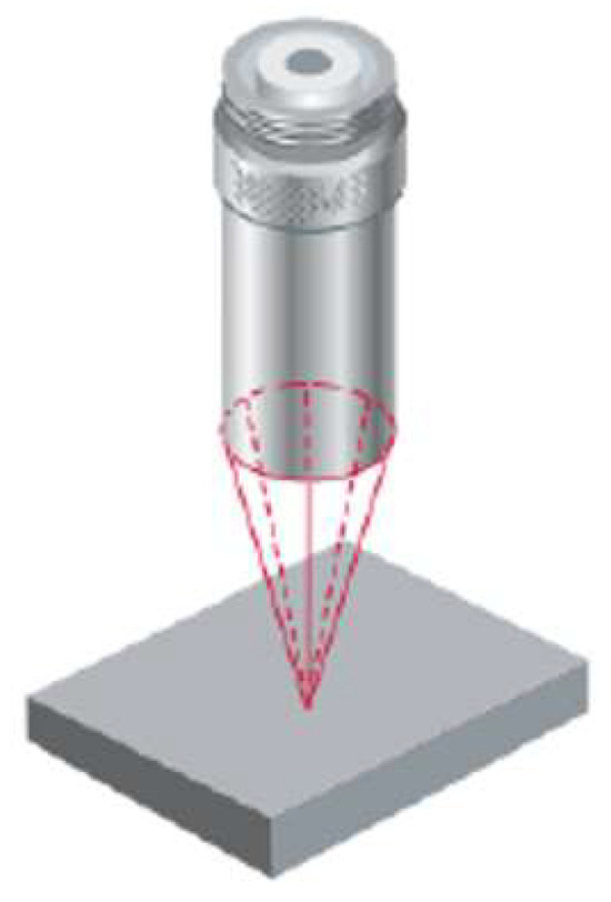
Figure 24.
An ultrasound probe with a spherical lens and a cone of ultrasonic waves.
An immersion-type, spherical-focus pulse-echo transducer (0.375″ element diameter, 4″ focal length) with a nominal center frequency of 10 MHz and UHF connector was used. It was coupled via an RG-174 cable to a UA463 pulser/receiver configured with 500 Ω of damping, a 100 Vpp transmit voltage, an 8 dB attenuation, and a P/E gain of 20 (HPF/LPF off). This ultrasound probe is both a transmitter and a receiver, enabling diagnostics using a pulse-echo method. Depending on the angle of the ultrasonic wave propagation vector relative to the surface area of the scanned object, oblique and direct reverberation of the objects is distinguished using the ultrasonic pulse-echo method. This reverberation angle must be considered when displaying the measured data in both 2D and 3D views of defects.
A computer card that converts the analog sound signal into a digital one is used for digitizing the data. The digitized signal is visualized in a real-time graph, as shown in Figure 25. It is also stored in files with data on the current position of the ultrasound diagnostic robot.
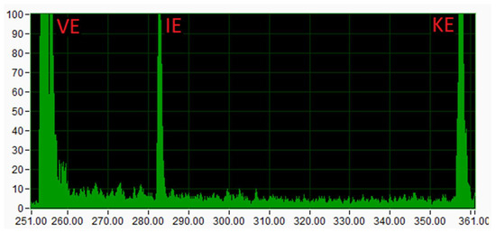
Figure 25.
Graph showing defect detection (IE) and input (VE) and output (KE) echo.
A so-called B scan was created from the data measured, saved in a file, and corrected depending on the angle of rotation of the probe. The graphic display shown in Figure 26 demonstrates the defect identification’s correctness. The graph in Figure 26 displays results from the pulse-echo method, characterized by multiple echoes. The structure of the object with known defects is shown in Figure 26 on the right. While comprehensive performance testing is still underway, the promise of our prototype is already evident. Figure 26 compares the measured defect signatures against their expected characteristics, demonstrating close alignment and suggesting that our approach can reliably distinguish known flaws.
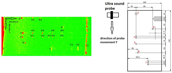
Figure 26.
Left: measured data with defects (red colored) displayed in B scan; Right: construction of known defect etalon.
The scheme of the dataflow among the ultrasonic measuring system, the robotic system, and the SW for monitoring the diagnostic process, archiving data, and viewing the results of defectoscopy is shown in Figure 27. Data collection from the ultrasound probe is realized by digitalizing the ultrasonic measurement with a USPC 7100 computer card Socomate, Crécy la Chapelle, France directly into the software for monitoring the ultrasonic measurement. Probe positioning was performed with a KUKA KR 60-3 industrial robot (6 DOF), featuring a maximum arm payload of 60 kg, maximum reach of 2033 mm, and a pose repeatability of ±0.06 mm. The positioning of the effector of the ultrasonic robot to the desired distance from the diagnosed object is realized using feedback from three optoNCDT 1402 laser distance sensors. The optoNCDT ILD1402-200.013 uses a visible-red semiconductor laser (λ = 670 nm, ≤1 mW, Class 2) for triangulation-based distance measurement. It provides a 0–200 mm measuring range with a linearity deviation ≤ 0.18% FSO (≤360 µm) and an averaged resolution of 13 µm. The mentioned laser rangefinders are connected to the industrial robot via a 4-channel analog input terminal EL3154. Data on the current position of the effector are sent to the software for monitoring the diagnostic process from the control computer of the KUKA KRC4 robot.
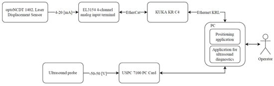
Figure 27.
Dataflow scheme for ultrasonic measurement and connection of robot controllers.
A part of the robotic ultrasound diagnostic system for non-destructive testing in highly variable production is software that enables real-time monitoring of the robotic ultrasound diagnostic process and storing measured data in files. At the same time, this software can view created archive files in a graphic display with defects clearly displayed in 3D. The monitoring and data archiving software of the robotic ultrasound diagnostic system for non-destructive testing in highly variable production is shown in Figure 28.
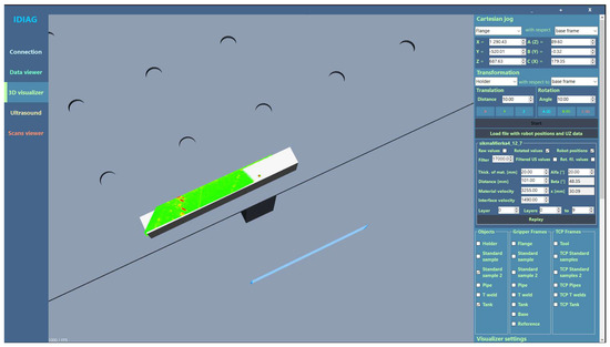
Figure 28.
Monitoring and data archiving software.
7. Validation of Defect Diagnostics in Robotic Ultrasound Diagnostic Workplace for Highly Variable Production
Experiments with several objects of different shapes and materials tested the ability to adapt to automated robotic testing of variable production. A T-shaped object and a cylindrical object are shown in Figure 12 and the video at https://youtu.be/bwcD-jNpSOU accessed on 14 May 2025. Experiments with another type of shape are shown in Figure 29.
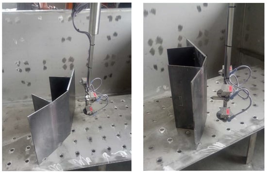
Figure 29.
Adaptation of the refracted surface by the automatic robotic positioning based on feedback from the laser distance sensor measurements.
Measurements of an object with the surface shown in Figure 30 tested the robotic ultrasound diagnostic workplace’s adaptation ability for highly variable production. Figure 31 shows the experimental measurement. The angular object’s surface and the robot’s average trajectory following the angular object’s surface are shown on the graph in Figure 32.
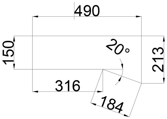
Figure 30.
Objects for the adaptation ability of the automatic robotic positioning measurement.
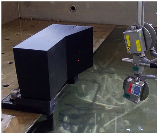
Figure 31.
Measurement for adaptation ability validation.
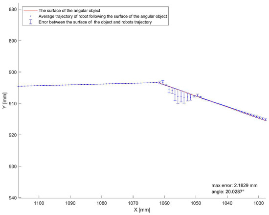
Figure 32.
A graph of the average trajectory of the robot following the angular surface of the diagnosed part.
According to the measured data presented in the graph in Figure 27, the maximum error is 2.18 mm. This error of robotic positioning in the experimented prototype is acceptable for ultrasound diagnostics in liquid because the first ultrasound echo allows us to precisely determine the position of the surface of the diagnosed object. The ability to diagnose defects was verified in the robotic ultrasound diagnostic system prototype for non-destructive testing in highly variable production using a metal etalon in the shape of a cuboid with three known internal defects. The construction of the etalon and the positions of the defects are shown in Figure 33.
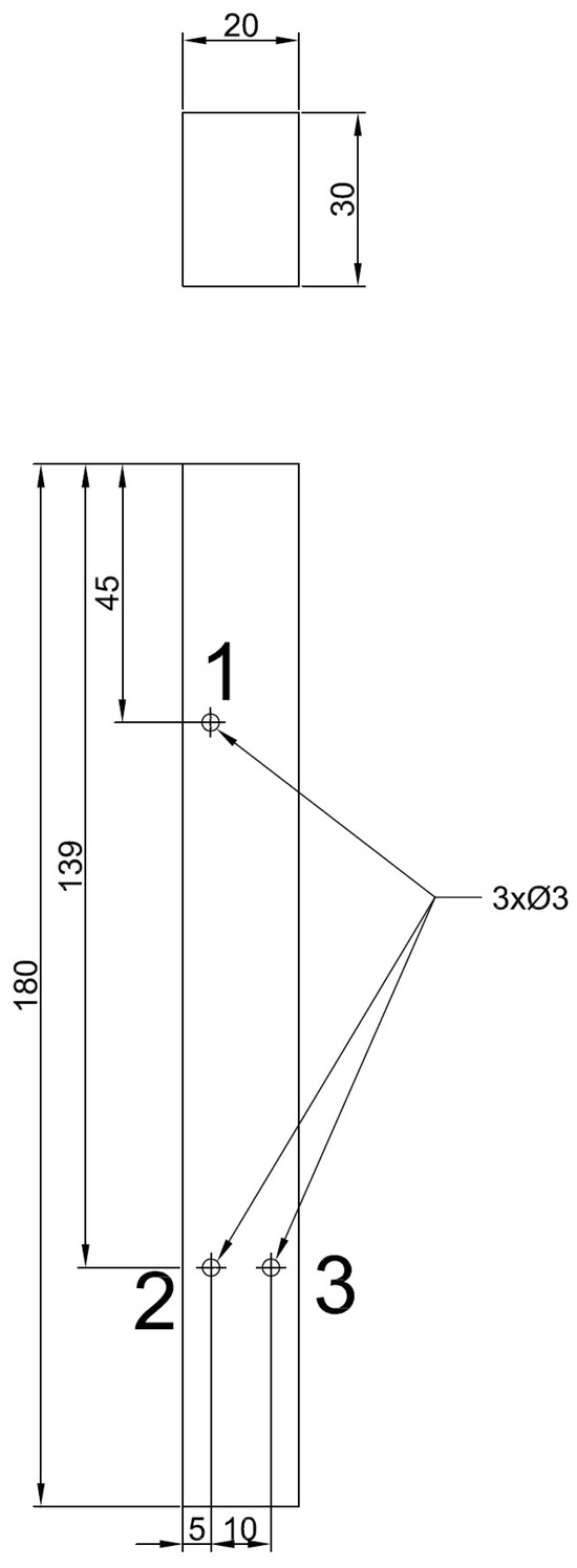
Figure 33.
Construction of validation etalon. 1—first internal defect, 2—second internal defect, 3—third internal defect.
During verification, the etalon was placed inside the diagnostic tank holder. The diagnostic ultrasound robot positioned the probe so the measurement covered the entire volume of interest. Measured data on the current position within the diagnosed site and the level of the reflected ultrasound signal were recorded in a file with the sample identifier. The measured data provide the data necessary to plot the diagnosed defects. The structure of the set of measured data is shown in Table 6, which shows information about Item Number, Layer, A-scan, US Measurement in A-Scan Item Number, US Measurement in dB, US Measurement Position X, US Measurement Position Y, US Measurement Position Z, Point Color RED, Point Color GREEN, and Point Color BLUE. Green-colored cells correspond to points without defects, and red-colored cells correspond to defects.
Table 6.
The part set of the ultrasound, position measurement, and color information of the point.
Data from the A-scan are combined with data on the position of the ultrasound diagnostic robot. The known positions of the diagnosed elemental volume of the analyzed volume are displayed for users in the graphic form of a 3D visualization of the measured data. In Figure 34, this robotic ultrasound data cloud is plotted along with parts of the diagnostic tank and the diagnostic robot’s effector.
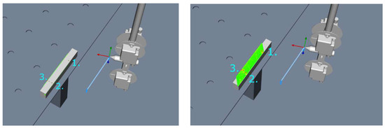
Figure 34.
(Left): etalon defect positions in 3D. (Right): diagnosed etalon defects in 3D color render.
Figure 34 on the left shows a reference with positions of the known defects. Figure 34 on the right shows a rendering from a 3D visualization of the measured data with a color differentiation of defects shown in red.
Video from the laboratory testing of the robotic ultrasound diagnostic using a collaborative robot and the sequence showed an example of the robotic ultrasound diagnostic system used in an actual robotic workplace with laser measurement for feedback positioning of the industrial diagnostic robot, which is available at https://www.vuez.sk/sluzba/robotika-a-digitalizacia/galerie#lightbox-videogallery5 accessed on 14 May 2025. This robotic workplace is used in the industry for robotic weld testing.
8. Conclusions
This paper describes the design, verification, and validation of the robotic ultrasound diagnostic system (Figure 35) for non-destructive testing in highly variable production.
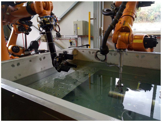
Figure 35.
This robotic ultrasound diagnostic system for non-destructive testing diagnoses a cylindrical object.
Highly variable production is characterized by a high degree of need to adjust the workplace due to the high variability of to-be-diagnosed objects. For this reason, the robotic ultrasound diagnostic system needs to be able to adjust itself automatically based on the shape and size of the object of the required type. A key feature of highly variable manufacturing is the ability to adapt as automatically as possible. To increase the ability to adapt to variable objects, robotic positioning equipped with a robotic gripper quick-change system and the robotic holding of the diagnosed object during the ultrasound diagnostic process was chosen for object manipulation. In addition to the robotic positioning of analyzed objects, the ultrasound probe is also positioned robotically. The computer control of robots allows for the generation of variable paths for robot positioning and diagnostics. For cylindrical objects, positioning through the seventh rotation axis of the diagnostic robot was designed into the system. At the same time, there is a space for diagnostics performed in a liquid environment inside the diagnostic tank equipped with a table to place the diagnosed objects. The ability to dynamically adapt to the shape and size of the currently diagnosed object was also increased by the implemented method of the ultrasound probe’s automatic robotic positioning based on measurements by laser distance sensors. To use it, it was necessary to design a robotic effector in such a way as to enable the simultaneous robotic positioning and functionality of three pieces of point laser scanners that measure the distance from the diagnosed object in a liquid environment. An ultrasound diagnostic probe was placed as part of the effector at the tool center point as a transmitter and receiver of an ultrasonic signal to provide data characterizing the homogeneity (quality) of the material under the scanned surface of the diagnosed object. Robotic positioning of the probe or simultaneous synchronized robotic positioning of the probe and the object was designed so that the signal from the ultrasound probe covered the entire area of interest. The oscillation was demonstrated when testing the effector of the ultrasound diagnostic robot. This led to the need to optimize robotic measurement effector design. The design of the robotic ultrasound diagnostic system for non-destructive testing in highly variable production was verified using a digital twin.
A calibration tool was created to achieve high measurement accuracy with a tip in the focal point corresponding to the probe type used. At the same time, it was necessary to calibrate the distance measurement sensors to obtain a transmission characteristic for the correction of laser distance measurements in the liquid environment of the diagnostic tank, according to Section 4. Subsequently, the calibration of the system of three scanners was carried out, which were placed in positions determined by the specific positions of the robotic effector and rotated by the required angle to the ultrasonic cone axis. The required rotation was realized thanks to three protractors attached to the robotic effector at the positions where the rangefinders were placed.
The measured data obtained by robotic positioning of the ultrasonic probe form a cloud of data that can be used for 3D visualization of the scanned object, its defects, and its classification.
The user software was created to set the parameters, display the measured data’s graphic progress in real-time, and visualize the identified defects in the analyzed object in 3D.
Verification of the ability to identify defects was validated by testing an etalon with known defects, as described in Section 7.
The present paper describes a robotic ultrasound diagnostic system for non-destructive testing in highly variable production suitable for use as an effective diagnostic tool in automated high-level output. Moreover, our work complements the immersion-based NDT approach of Kustroń et al. [1], who demonstrated the effectiveness of pseudo-surface ultrasonic waves and LS-DYNA-driven FEM simulations for the quality evaluation of MIAB-welded drive shafts. Whereas Kustroń et al. employed a fixed, water-immersed setup to characterize weld defects, our contactless, robotically guided pulse-echo system enables fully automated scanning and adaptive path planning in a prototype cell. Together, these two methodologies underscore the broad promise of ultrasonic NDT—combining rigorous physical modeling with robotic flexibility to advance inline inspection in high-variability manufacturing.
Robotic ultrasonic diagnostics can be used in industrial processes for the internal quality control of objects as well as the thickness of materials. Compared to X-ray quality testing, its advantage is reducing the risk of exposure to workers and removing investment costs required to build barriers around the radiation source. The speed of the robot’s movement and, thus, the cycle time of the diagnostic process depends on the requirements for the distinguishing ability of the examined defects, which was the subject of the experiments described in Section 6.
The time required for the robotic positioning of the ultrasound probe can be reduced by using phased array probes. These probes can scan a larger volume of material of the diagnosed object per unit of time and reduce the wear of the robotic arm. Following this publication, research and development activities will focus on these issues.
Author Contributions
Conceptualization, Z.K. and M.R.; Methodology, L.C.; Software, M.P. and E.S.; Validation, M.T.; Investigation, M.P.; Data curation, E.S.; Writing—original draft, Z.K. and M.T.; Writing—review & editing, M.R.; Supervision, F.D.; Funding acquisition, Z.K. All authors have read and agreed to the published version of the manuscript.
Funding
This work was supported by the Operational Program Integrated Infrastructure for the project: “Digitisation of Robotised Welding Workplace (DIROZ)”, code ITMS2014 +: 313012S686.
Data Availability Statement
Data are contained within the article.
Conflicts of Interest
Authors Zuzana Kovarikova, Martin Porubsky, Marek Trebula and Eva Salat were employed by the company VUEZ, a.s. The remaining authors declare that the research was conducted in the absence of any commercial or financial relationships that could be construed as a potential conflict of interest.
References
- Kustroń, P.; Korzeniowski, M.; Piwowarczyk, T.; Sokołowski, P. Application of Immersion Ultrasonic Testing for Non-Contact Quality Evaluation of Magnetically Impelled Arc Butt Welded Drive Shafts of Motor Vehicles. Adv. Automob. Eng. 2017, 6, 161. [Google Scholar] [CrossRef]
- Lofving, M.; Almstrom, P.; Jarebrant, C.; Wadman, B.; Widfeldt, M. Evaluation of flexible automation for small batch production. Procedia Manuf. 2018, 25, 177–184. [Google Scholar] [CrossRef]
- Ilesanmi, A.D.; Moses, O.; Khumbulani, M.; Samuel, O.N. Application of the Fourth Industrial Revolution for High Volume Production in the Rail Car Industry. Mass Prod. Process. 2019. [Google Scholar] [CrossRef]
- Halim, N.N.A.; Shariff, S.S.R.; Zahari, S.M. Modeling an Automobile Assembly Layout Plant Using Probabilistic Functions and Discrete Event Simulation. In Proceedings of the International Conference on Industrial Engineering and Operations Management, Detroit, MI, USA, 10–14 August 2020; Volume 5, pp. 2726–2737. [Google Scholar]
- Kampker, A.; Hollah, A.; Triebs, J.; Löffler, B. Modular Body Shop with Process-and Component-integrated Jig Features. ATZ Prod. Worldw. 2019, 6, 10–15. [Google Scholar] [CrossRef]
- Ensminger, D.; Stulen, F.B. Ultrasonics. Data, Equations, and Their Practical Uses; CRC Press Taylor & Francis Group: Boca Raton, FL, USA, 2009; Volume 366, pp. 371–372. [Google Scholar]
- Madhumitha, P.; Ramkishore, S.; Srikanth, K.S.; Palanichamy, P. Application of Decision Trees for the Identification of Weld Central Line in Austenitic Stainless Steel Weld joints. In Proceedings of the 2014 International Conference on Computation of Power, Energy, Information and Communication (TCCPETC), Chennai, India, 16–17 April 2014. [Google Scholar] [CrossRef]
- Spong, M.W.; Hutchinson, S.; Vidyasagar, M. Robot Modeling and Control; Wiley: Hoboken, NJ, USA, 2005; pp. 7–8. [Google Scholar]
- Bologna, F.; Tannous, M.; Romano, D.; Stefanini, C. Automatic welding imperfections detection in a smart factory via 2-D laser scanner. J. Manuf. Process. 2022, 73, 948–960. [Google Scholar] [CrossRef]
- Kovarikova, Z.; Porubsky, M.; Nagy, F.; Labat, D.; Bachorik, O.; Duchon, F.; Babinec, A.; Chovanec, L.; Stalmachova, E.; Dekan, M. System of Intelligent Robotic Ultrasound Diagnostics; EWSPAPER 2021; Office of Industrial Property of the Slovak Republic: Banska Bystrica, Slovak Republic, 2021. [Google Scholar]
- Liu, C.; Jiang, P.; Jiang, W. Web-based digital twin modeling and remote control of cyber-physical production systems. Robot. Comput.-Integr. Manuf. 2020, 64, 101956. [Google Scholar] [CrossRef]
- Ferro, R.; Sajjad, H.; Ordonez, R.E.C. Steps for Data Exchange between Real Environment and Virtual Simulation Environment. In Proceedings of the ICCMS 2021, Melbourne, VIC, Australia, 25–27 June 2021. [Google Scholar]
- Dumic, E.; Battisti, F.; Carli, M.; Silva Cruz, L.A. Point Cloud Visualization Methods: A Study on Subjective Preferences. In Proceedings of the 2020 28th European Signal Processing Conference (EUSIPCO), Amsterdam, The Netherlands, 18–21 January 2020. [Google Scholar] [CrossRef]
Disclaimer/Publisher’s Note: The statements, opinions and data contained in all publications are solely those of the individual author(s) and contributor(s) and not of MDPI and/or the editor(s). MDPI and/or the editor(s) disclaim responsibility for any injury to people or property resulting from any ideas, methods, instructions or products referred to in the content. |
© 2025 by the authors. Licensee MDPI, Basel, Switzerland. This article is an open access article distributed under the terms and conditions of the Creative Commons Attribution (CC BY) license (https://creativecommons.org/licenses/by/4.0/).