
Scalable Multi-Robot Task Allocation Using Graph Deep Reinforcement Learning with Graph Normalization
 , , ,
, , ,
Abstract
1. Introduction
2. Related Works
2.1. Traditional MRTA Solutions
2.2. DRL-Based Methods
3. Problem Formulation
4. Methodology
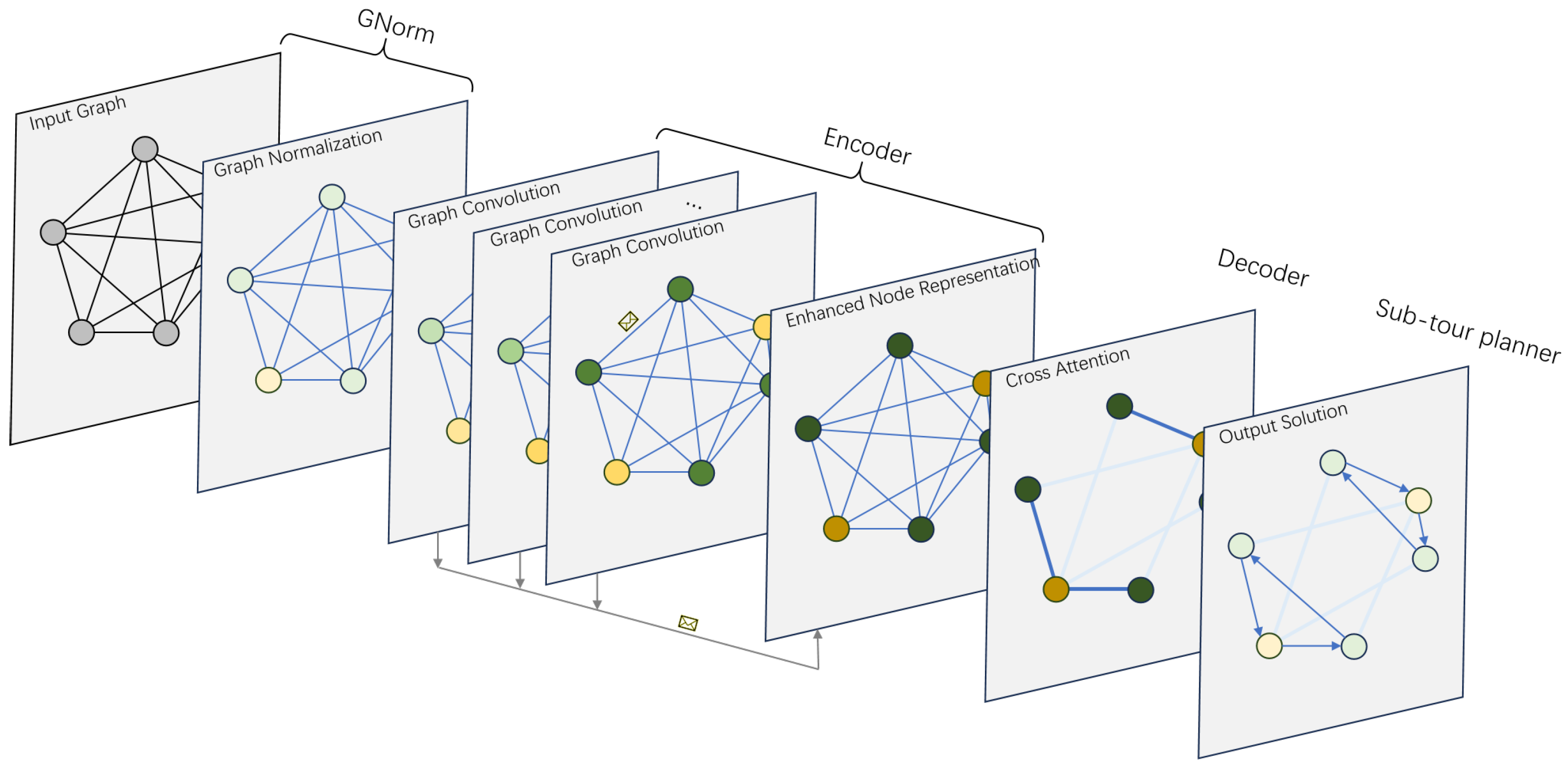
4.1. Policy Network Architecture
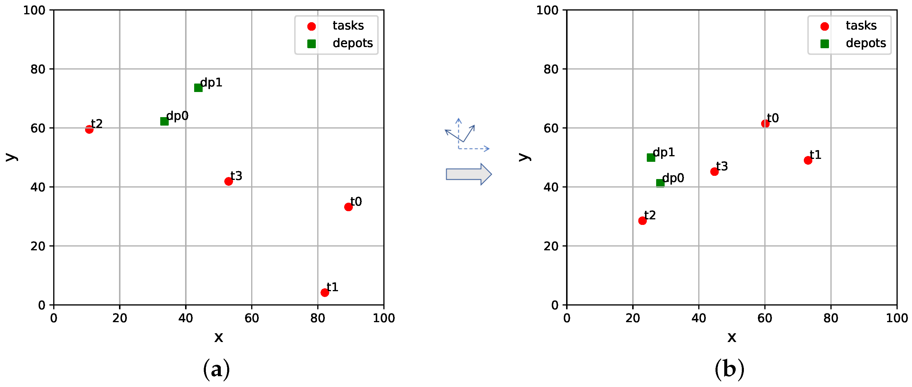
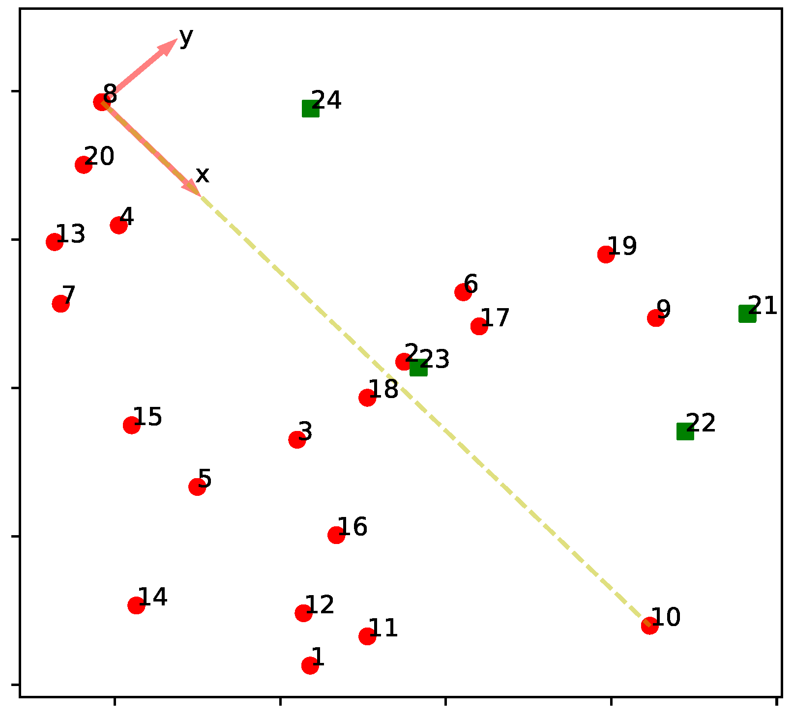
4.2. Graph Normalization
4.3. Encoder
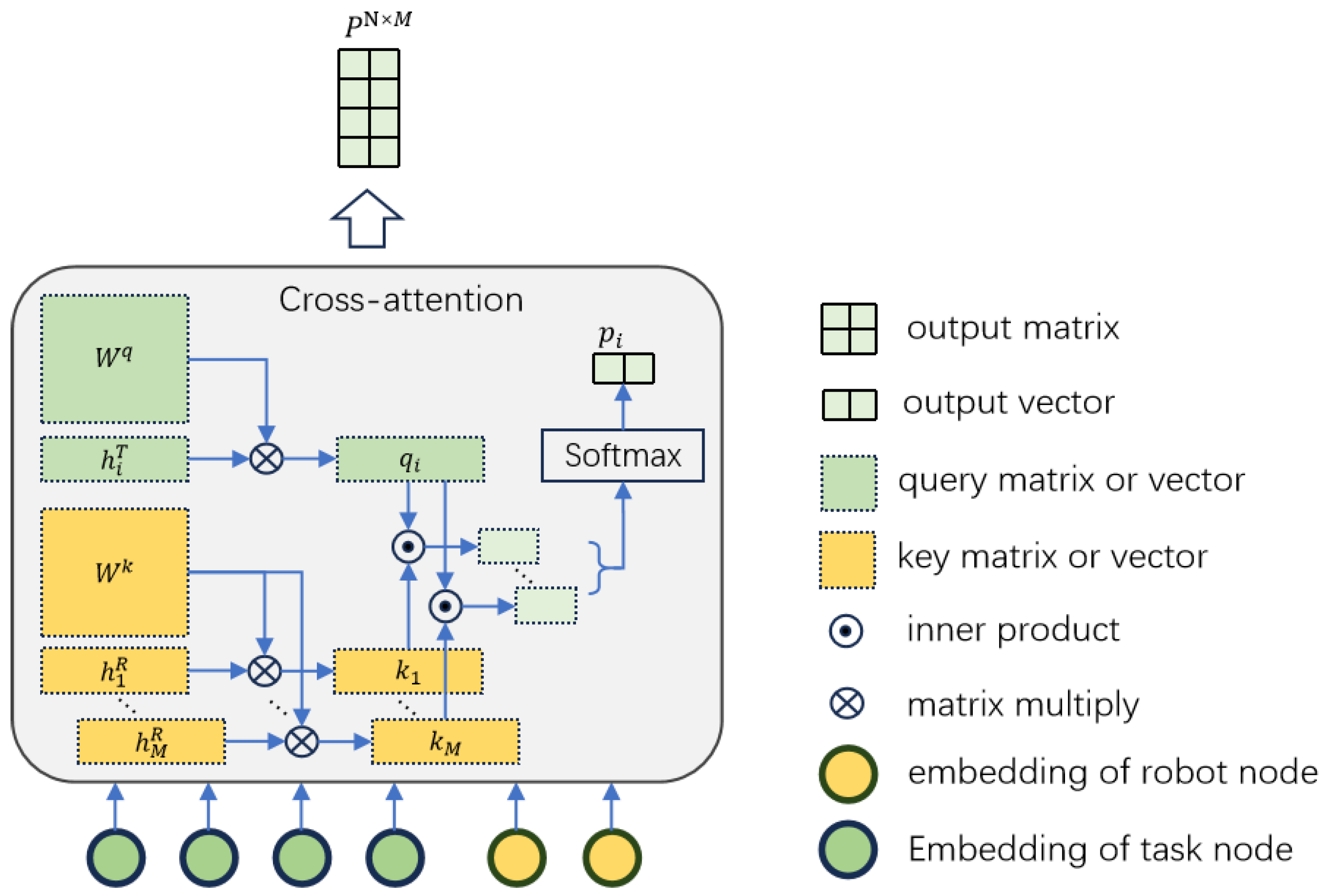
4.4. Decoder
4.5. Training
| Algorithm 1: Training a policy network with the bootstrapping REINFORCE algorithm for MRTA |
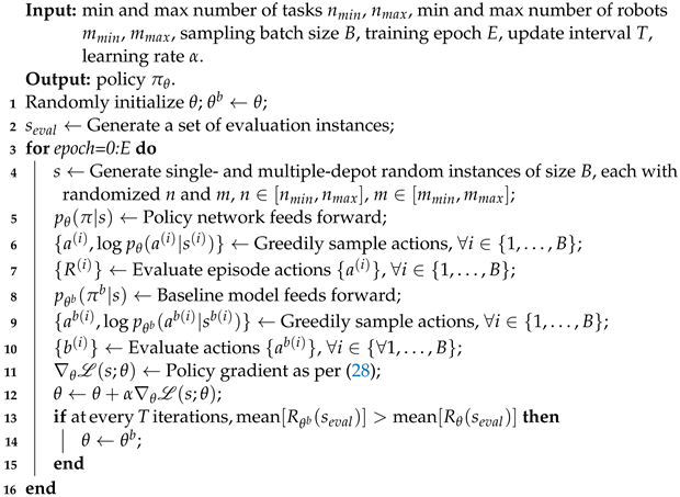 |
5. Simulation
5.1. Experimental Set-Up
- A heuristic algorithm, which is realized by OR-TOOLS [41].
- A meta-heuristic algorithm, the GA in this paper.
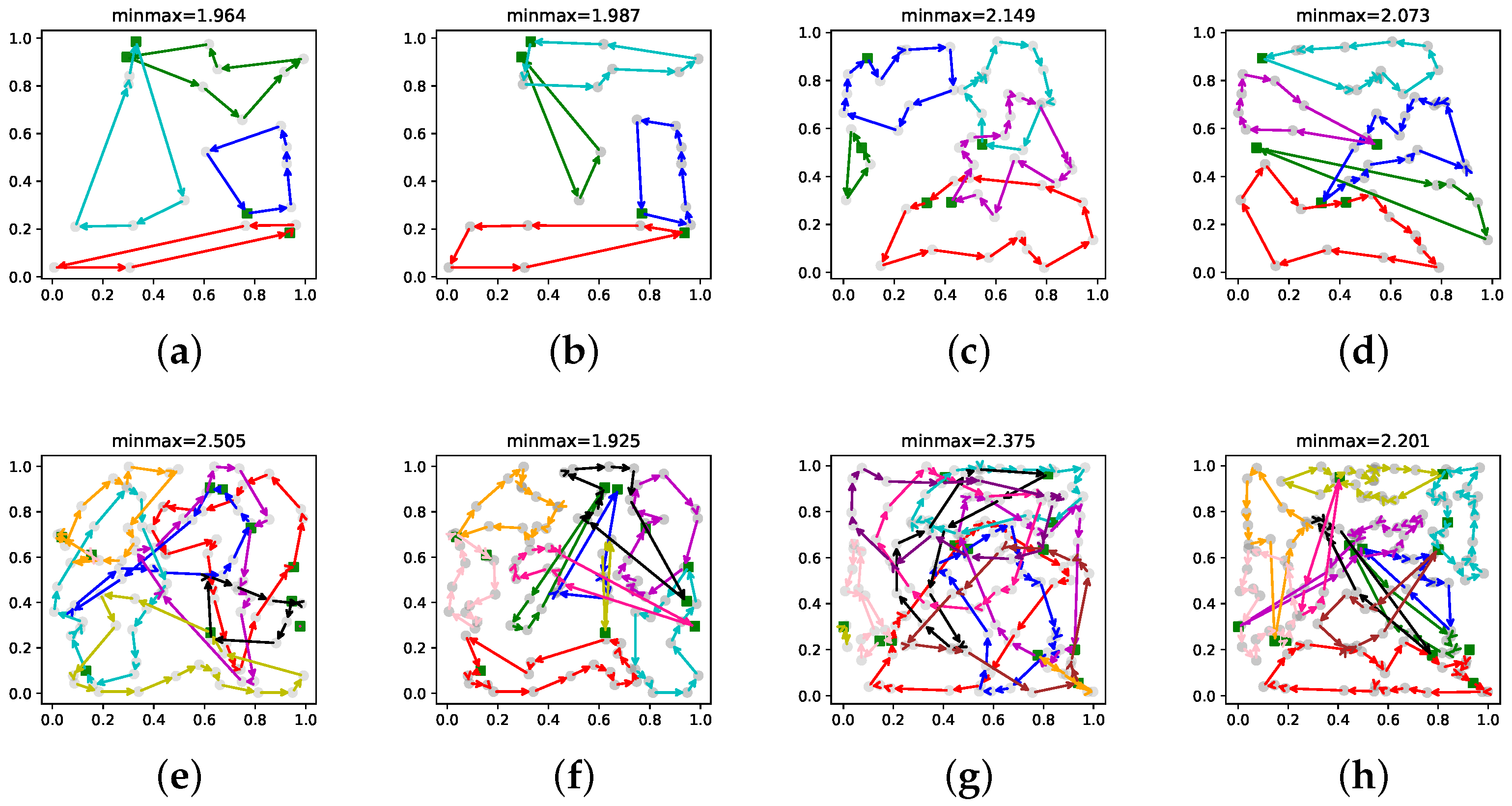
5.2. Testing on Single-Depot MRTA
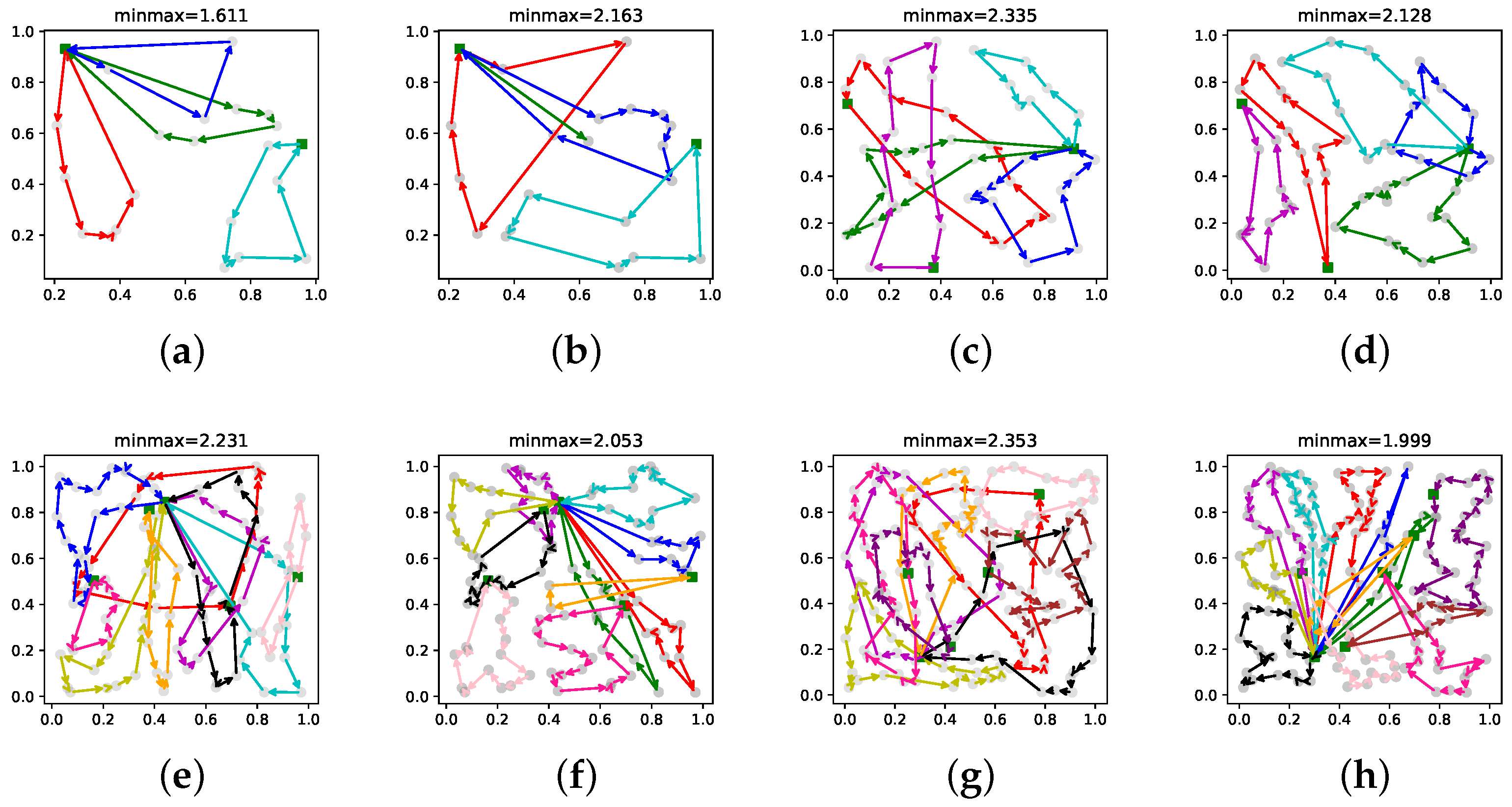
5.3. Testing on Multiple-Depot MRTA
6. Discussion
7. Conclusions
Author Contributions
Funding
Data Availability Statement
Conflicts of Interest
Abbreviations
| DAN | Decentralized Attention Neural Network |
| DisPN | Distributed Policy Network |
| DRL | Deep Reinforcement Learning |
| GA | Genetic Algorithm |
| GraphSAGE | Graph SAmple and aggreGatE |
| LKH | Lin–Kernighan–Helsgaun |
| MD-MRTA | Multiple-Depot Multi-Robot Task Allocation |
| MLP | Multiple Layer Perception |
| MRS | Multi-Robot System |
| MSMD-MRTA | Mixed Single- and Multiple-Depot Multi-Robot Task Allocation |
| MRTA | Multi-Robot Task Allocation |
| mTSP | Multiple Traveling Salesman Problem |
| SD-MRTA | Single-Depot Multi-Robot Task Allocation |
References
- Verma, J.K.; Ranga, V. Multi-robot coordination analysis, taxonomy, challenges and future scope. J. Intell. Robot. Syst. 2021, 102, 10. [Google Scholar] [CrossRef] [PubMed]
- Khamis, A.; Hussein, A.; Elmogy, A. Multi-robot task allocation: A review of the state-of-the-art. In Cooperative Robots and Sensor Networks 2015; Springer: Cham, Switzerland, 2015; pp. 31–51. [Google Scholar]
- Gerkey, B.P.; Matarić, M.J. A formal analysis and taxonomy of task allocation in multi-robot systems. Int. J. Robot. Res. 2004, 23, 939–954. [Google Scholar] [CrossRef]
- Korsah, G.A.; Stentz, A.; Dias, M.B. A comprehensive taxonomy for multi-robot task allocation. Int. J. Robot. Res. 2013, 32, 1495–1512. [Google Scholar] [CrossRef]
- Liu, H.; Li, X.; Wu, G.; Fan, M.; Wang, R.; Gao, L.; Pedrycz, W. An iterative two-phase optimization method based on divide and conquer framework for integrated scheduling of multiple UAVs. IEEE Trans. Intell. Transp. Syst. 2020, 22, 5926–5938. [Google Scholar] [CrossRef]
- Liu, Y.; Song, R.; Bucknall, R.; Zhang, X. Intelligent multi-task allocation and planning for multiple unmanned surface vehicles (USVs) using self-organising maps and fast marching method. Inf. Sci. 2019, 496, 180–197. [Google Scholar] [CrossRef]
- Zhou, B.; Zhou, R.; Gan, Y.; Fang, F.; Mao, Y. Multi-robot multi-station cooperative spot welding task allocation based on stepwise optimization: An industrial case study. Robot. Comput.-Integr. Manuf. 2022, 73, 102197. [Google Scholar] [CrossRef]
- Jose, K.; Pratihar, D.K. Task allocation and collision-free path planning of centralized multi-robots system for industrial plant inspection using heuristic methods. Robot. Auton. Syst. 2016, 80, 34–42. [Google Scholar] [CrossRef]
- Zheng, H.; Yuan, J. An Integrated Mission Planning Framework for Sensor Allocation and Path Planning of Heterogeneous Multi-UAV Systems. Sensors 2021, 21, 3557. [Google Scholar] [CrossRef]
- Wang, Q.; Tang, C. Deep reinforcement learning for transportation network combinatorial optimization: A survey. Knowl.-Based Syst. 2021, 233, 107526. [Google Scholar] [CrossRef]
- Mahmud, M.S.A.; Abidin, M.S.Z.; Buyamin, S.; Emmanuel, A.A.; Hasan, H.S. Multi-objective route planning for underwater cleaning robot in water reservoir tank. J. Intell. Robot. Syst. 2021, 101, 9. [Google Scholar] [CrossRef]
- Yan, M.; Yuan, H.; Xu, J.; Yu, Y.; Jin, L. Task allocation and route planning of multiple UAVs in a marine environment based on an improved particle swarm optimization algorithm. EURASIP J. Adv. Signal Process. 2021, 2021, 94. [Google Scholar] [CrossRef]
- Kool, W.; Van Hoof, H.; Welling, M. Attention, learn to solve routing problems! In Proceedings of the 7th International Conference on Learning Representations. ICLR, New Orleans, LA, USA, 6–9 May 2019; IEEE: Piscataway, NJ, USA, 2019; pp. 1–25. [Google Scholar]
- Wang, L.; Hu, X.; Wang, Y.; Xu, S.; Ma, S.; Yang, K.; Liu, Z.; Wang, W. Dynamic job-shop scheduling in smart manufacturing using deep reinforcement learning. Comput. Netw. 2021, 190, 107969. [Google Scholar] [CrossRef]
- Hu, Y.; Yao, Y.; Lee, W.S. A reinforcement learning approach for optimizing multiple traveling salesman problems over graphs. Knowl.-Based Syst. 2020, 204, 106244. [Google Scholar] [CrossRef]
- Cao, Y.; Sun, Z.; Sartoretti, G. Dan: Decentralized attention-based neural network to solve the minmax multiple traveling salesman problem. arXiv 2021, arXiv:2109.04205. [Google Scholar]
- Chakraa, H.; Guérin, F.; Leclercq, E.; Lefebvre, D. Optimization techniques for Multi-Robot Task Allocation problems: Review on the state-of-the-art. Robot. Auton. Syst. 2023, 168, 104492. [Google Scholar] [CrossRef]
- Karmani, R.K.; Latvala, T.; Agha, G. On scaling multi-agent task reallocation using market-based approach. In Proceedings of the First International Conference on Self-Adaptive and Self-Organizing Systems (SASO 2007), Cambridge, MA, USA, 9–11 July 2007; IEEE: Piscataway, NJ, USA, 2007; pp. 173–182. [Google Scholar]
- Koubâa, A.; Cheikhrouhou, O.; Bennaceur, H.; Sriti, M.F.; Javed, Y.; Ammar, A. Move and improve: A market-based mechanism for the multiple depot multiple travelling salesmen problem. J. Intell. Robot. Syst. 2017, 85, 307–330. [Google Scholar] [CrossRef]
- Choi, H.L.; Brunet, L.; How, J.P. Consensus-based decentralized auctions for robust task allocation. IEEE Trans. Robot. 2009, 25, 912–926. [Google Scholar] [CrossRef]
- Brunet, L.; Choi, H.L.; How, J. Consensus-based auction approaches for decentralized task assignment. In Proceedings of the AIAA Guidance, Navigation and Control Conference and Exhibit, Honolulu, HI, USA, 18–21 August 2008; p. 6839. [Google Scholar]
- Zhao, W.; Meng, Q.; Chung, P.W. A heuristic distributed task allocation method for multivehicle multitask problems and its application to search and rescue scenario. IEEE Trans. Cybern. 2015, 46, 902–915. [Google Scholar] [CrossRef] [PubMed]
- Geng, N.; Meng, Q.; Gong, D.; Chung, P.W. How good are distributed allocation algorithms for solving urban search and rescue problems? A comparative study with centralized algorithms. IEEE Trans. Autom. Sci. Eng. 2018, 16, 478–485. [Google Scholar] [CrossRef]
- Wang, Z.; Wang, B.; Wei, Y.; Liu, P.; Zhang, L. Cooperative multi-task assignment of multiple UAVs with improved genetic algorithm based on beetle antennae search. In Proceedings of the 2020 39th Chinese Control Conference (CCC), Shenyang, China, 27–29 July 2020; IEEE: Piscataway, NJ, USA, 2020; pp. 1605–1610. [Google Scholar]
- Chen, K.; Sun, Q.; Zhou, A.; Wang, S. Adaptive multiple task assignments for uavs using discrete particle swarm optimization. In Proceedings of the Internet of Vehicles. Technologies and Services Towards Smart City: 5th International Conference, IOV 2018, Paris, France, 20–22 November 2018; Proceedings 5. Springer: Berlin/Heidelberg, Germany, 2018; pp. 220–229. [Google Scholar]
- Zitouni, F.; Harous, S.; Maamri, R. A distributed approach to the multi-robot task allocation problem using the consensus-based bundle algorithm and ant colony system. IEEE Access 2020, 8, 27479–27494. [Google Scholar] [CrossRef]
- Venkatesh, P.; Singh, A. Two metaheuristic approaches for the multiple traveling salesperson problem. Appl. Soft Comput. 2015, 26, 74–89. [Google Scholar] [CrossRef]
- Zhou, H.; Song, M.; Pedrycz, W. A comparative study of improved GA and PSO in solving multiple traveling salesmen problem. Appl. Soft Comput. 2018, 64, 564–580. [Google Scholar] [CrossRef]
- Dong, Y.; Wu, Q.; Wen, J. An improved shuffled frog-leaping algorithm for the minmax multiple traveling salesman problem. Neural Comput. Appl. 2021, 33, 17057–17069. [Google Scholar] [CrossRef]
- Mahmoudinazlou, S.; Kwon, C. A hybrid genetic algorithm for the min–max Multiple Traveling Salesman Problem. Comput. Oper. Res. 2024, 162, 106455. [Google Scholar] [CrossRef]
- Zhang, Y.; Han, X.; Dong, Y.; Xie, J.; Xie, G.; Xu, X. A novel state transition simulated annealing algorithm for the multiple traveling salesmen problem. J. Supercomput. 2021, 77, 11827–11852. [Google Scholar] [CrossRef]
- Vinyals, O.; Fortunato, M.; Jaitly, N. Pointer networks. Adv. Neural Inf. Process. Syst. 2015, 28, 2692–2700. [Google Scholar]
- Bello, I.; Pham, H.; Le, Q.V.; Norouzi, M.; Bengio, S. Neural combinatorial optimization with reinforcement learning. In Proceedings of the International Conference on Machine Learning (Workshop), Sydney, Australia, 6–11 August 2017. [Google Scholar]
- Wu, Y.; Song, W.; Cao, Z.; Zhang, J.; Lim, A. Learning improvement heuristics for solving routing problems. IEEE Trans. Neural Netw. Learn. Syst. 2021, 33, 5057–5069. [Google Scholar] [CrossRef] [PubMed]
- Ling, Z.; Zhang, Y.; Chen, X. A Deep Reinforcement Learning Based Real-Time Solution Policy for the Traveling Salesman Problem. IEEE Trans. Intell. Transp. Syst. 2023, 24, 5871–5882. [Google Scholar] [CrossRef]
- Gao, H.; Zhou, X.; Xu, X.; Lan, Y.; Xiao, Y. AMARL: An Attention-Based Multiagent Reinforcement Learning Approach to the Min-Max Multiple Traveling Salesmen Problem. IEEE Trans. Neural Netw. Learn. Syst. 2023; early access. [Google Scholar] [CrossRef]
- Bektas, T. The multiple traveling salesman problem: An overview of formulations and solution procedures. Omega 2006, 34, 209–219. [Google Scholar] [CrossRef]
- Hamilton, W.; Ying, Z.; Leskovec, J. Inductive representation learning on large graphs. Adv. Neural Inf. Process. Syst. 2017, 30, 1024–1034. [Google Scholar]
- Helsgaun, K. An effective implementation of the Lin–Kernighan traveling salesman heuristic. Eur. J. Oper. Res. 2000, 126, 106–130. [Google Scholar] [CrossRef]
- Necula, R.; Breaban, M.; Raschip, M. Tackling the bi-criteria facet of multiple traveling salesman problem with ant colony systems. In Proceedings of the 2015 IEEE 27th International Conference on Tools with Artificial Intelligence (ICTAI), Vietri sul Mare, Italy, 9–11 November 2015; IEEE: Piscataway, NJ, USA, 2015; pp. 873–880. [Google Scholar]
- Perron, L.; Furnon, V. ORTOOLS. 2020. Available online: https://developers.google.com/optimization/ (accessed on 16 April 2024).
- Shuai, Y.; Yunfeng, S.; Kai, Z. An effective method for solving multiple travelling salesman problem based on NSGA-II. Syst. Sci. Control Eng. 2019, 7, 108–116. [Google Scholar] [CrossRef]
- Pisinger, D.; Ropke, S. Handbook of Metaheuristics; Springer: Berlin/Heidelberg, Germany, 2019. [Google Scholar]


| Approaches | ||||||||
|---|---|---|---|---|---|---|---|---|
| Minmax | CPU Time (s) | Minmax | CPU Time (s) | Minmax | CPU Time (s) | Minmax | CPU Time (s) | |
| OR-TOOLS | 2.121 | 0.905 | 2.026 | 0.966 | 2.414 | 9.908 | 2.195 | 10.061 |
| GA | 2.590 | 3.624 | 2.482 | 3.991 | 3.246 | 8.803 | 2.921 | 12.257 |
| DisPN 1 | 2.143 | 0.024 | 1.995 | 0.027 | 2.493 | 0.048 | 2.135 | 0.044 |
| DAN 1 | 2.314 | 0.192 | 2.037 | 0.240 | 2.729 | 0.449 | 2.181 | 0.486 |
| gnPN | 2.174 | 0.001 | 1.955 | 0.001 | 2.484 | 0.003 | 2.068 | 0.004 |
| Approach | ||||||||
|---|---|---|---|---|---|---|---|---|
| Minmax | CPU Time (s) | Minmax | CPU Time (s) | Minmax | CPU Time (s) | Minmax | CPU Time (s) | |
| OR-TOOLS | 2.919 | 139.011 | 2.647 | 132.914 | 2.772 | 129.144 | 9.850 | 180 |
| GA | 4.444 | 22.431 | 3.855 | 29.459 | 3.742 | 32.542 | 7.344 | 83.183 |
| DisPN 1 | 3.210 | 0.201 | - | - | 2.436 | 0.161 | 4.891 | 0.933 |
| DAN | 3.414 | 1.819 | 2.628 | 1.772 | 2.420 | 1.786 | 5.342 | 15.502 |
| gnPN | 3.083 | 0.045 | 2.387 | 0.028 | 2.261 | 0.026 | 4.244 | 0.265 |
| minmax | CPU time (s) | minmax | CPU time (s) | minmax | CPU time (s) | minmax | CPU time (s) | |
| 9.918 | 180 | 9.923 | 180 | 14.787 | 180 | 14.869 | 180 | |
| 6.296 | 99.761 | 5.879 | 103.249 | 10.010 | 165.935 | 8.617 | 174.628 | |
| - | - | 3.340 | 0.537 | 6.377 | 2.575 | - | - | |
| 3.806 | 15.576 | 3.309 | 15.757 | 7.327 | 61.359 | 5.034 | 61.096 | |
| 3.251 | 0.179 | 2.941 | 0.153 | 5.195 | 0.697 | 3.895 | 0.469 | |
| minmax | CPU time (s) | minmax | CPU time (s) | minmax | CPU time (s) | minmax | CPU time (s) | |
| 14.793 | 180 | 18.364 | 180 | 18.368 | 180 | 14.853 | 180 | |
| 8.181 | 180 | 12.524 | 180 | 10.847 | 180 | 10.397 | 180 | |
| 4.304 | 1.406 | 7.432 | 4.428 | - | - | 4.986 | 2.366 | |
| 4.196 | 61.641 | 8.751 | 119.120 | 5.841 | 119.117 | 4.868 | 119.209 | |
| 3.474 | 0.390 | 5.810 | 1.128 | 4.282 | 0.729 | 3.831 | 0.639 | |
Disclaimer/Publisher’s Note: The statements, opinions and data contained in all publications are solely those of the individual author(s) and contributor(s) and not of MDPI and/or the editor(s). MDPI and/or the editor(s) disclaim responsibility for any injury to people or property resulting from any ideas, methods, instructions or products referred to in the content. |
© 2024 by the authors. Licensee MDPI, Basel, Switzerland. This article is an open access article distributed under the terms and conditions of the Creative Commons Attribution (CC BY) license (https://creativecommons.org/licenses/by/4.0/).
Share and Cite
Zhang, Z.; Jiang, X.; Yang, Z.; Ma, S.; Chen, J.; Sun, W. Scalable Multi-Robot Task Allocation Using Graph Deep Reinforcement Learning with Graph Normalization. Electronics 2024, 13, 1561. https://doi.org/10.3390/electronics13081561
Zhang Z, Jiang X, Yang Z, Ma S, Chen J, Sun W. Scalable Multi-Robot Task Allocation Using Graph Deep Reinforcement Learning with Graph Normalization. Electronics. 2024; 13(8):1561. https://doi.org/10.3390/electronics13081561
Chicago/Turabian StyleZhang, Zhenqiang, Xiangyuan Jiang, Zhenfa Yang, Sile Ma, Jiyang Chen, and Wenxu Sun. 2024. "Scalable Multi-Robot Task Allocation Using Graph Deep Reinforcement Learning with Graph Normalization" Electronics 13, no. 8: 1561. https://doi.org/10.3390/electronics13081561
APA StyleZhang, Z., Jiang, X., Yang, Z., Ma, S., Chen, J., & Sun, W. (2024). Scalable Multi-Robot Task Allocation Using Graph Deep Reinforcement Learning with Graph Normalization. Electronics, 13(8), 1561. https://doi.org/10.3390/electronics13081561