A Comparative Analysis of Computational Intelligence Methods for Autonomous Navigation of Smart Ships

Abstract

This paper presents the author’s approaches based on computational intelligence methods for application in the Autonomous Navigation System (ANS) of a smart ship. The considered task is collision avoidance, which is one of the vital functions of the ANS. The proposed methods, applying the Ant Colony Optimization and the Firefly Algorithm, were compared with other artificial intelligence approaches introduced in the recent literature, e.g., evolutionary algorithms and machine learning. The advantages and disadvantages of different algorithms are formulated. Results of simulation experiments carried out with the use of the developed algorithms are presented and discussed. Future trends and challenges of presented smart technologies are also stated.

1. Introduction

The development of smart technologies also relates to the maritime industry. Smart ships are vessels that use novel technologies in order to enhance their operation efficiency and safety of navigation. They use a vast number of various sensors in order to automate many processes connected with ship navigation, such as voyage planning or prediction of the ship’s systems and devices maintenance. Smart vessels also possess solutions for remote monitoring and decision-making from shore control centers.

An important issue in the development of smart ship technology is related to autonomous navigation systems, which utilize different sensors and systems such as AIS, ECDIS, GPS and radar with ARPA, and advanced control algorithms in order to assure safer and more efficient navigation. The collision avoidance system constitutes a vital part of an autonomous navigation system. The aim of the research presented in this paper is the development of effective and reliable algorithms, utilizing computational intelligence optimization methods, for application in a collision avoidance system.

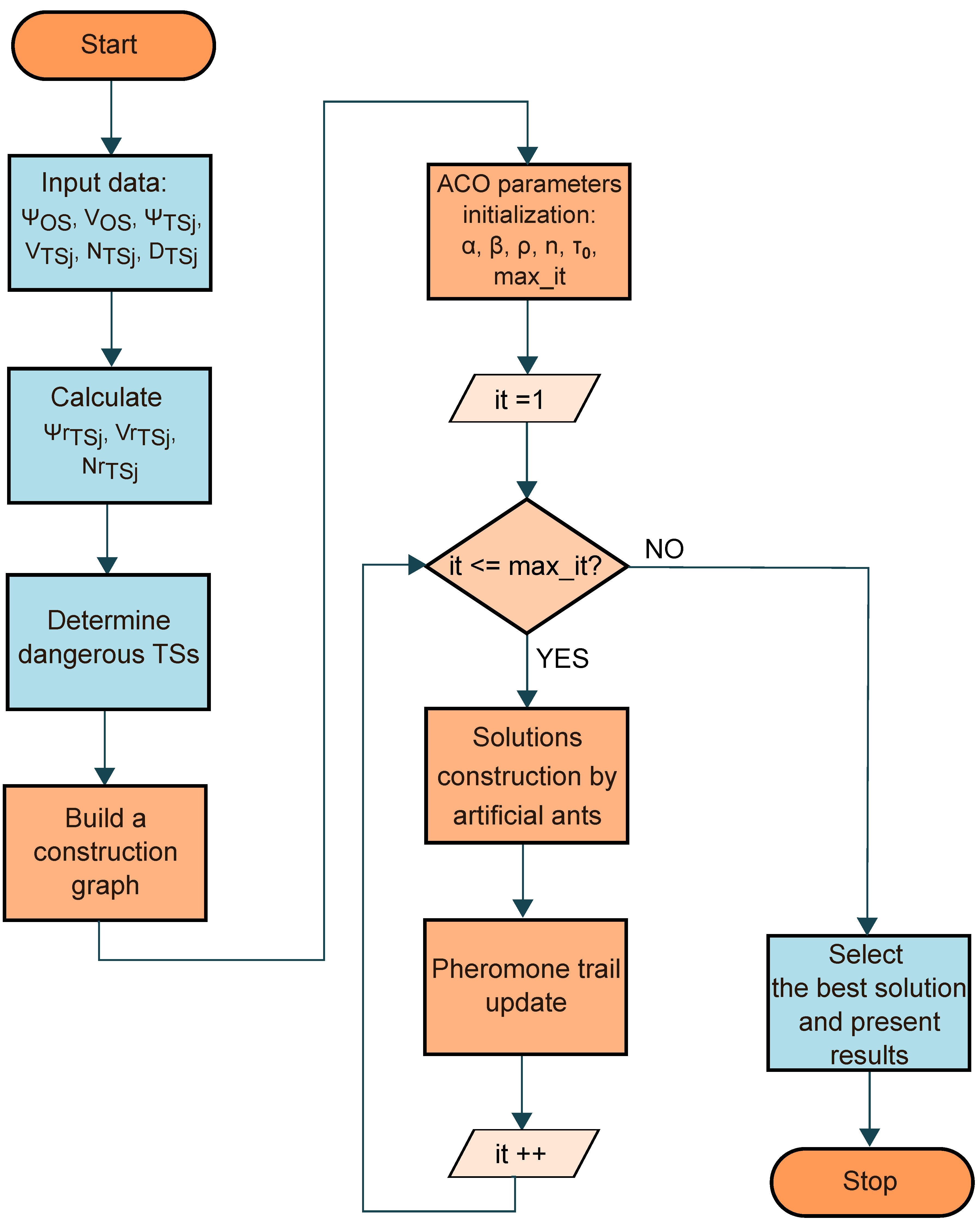
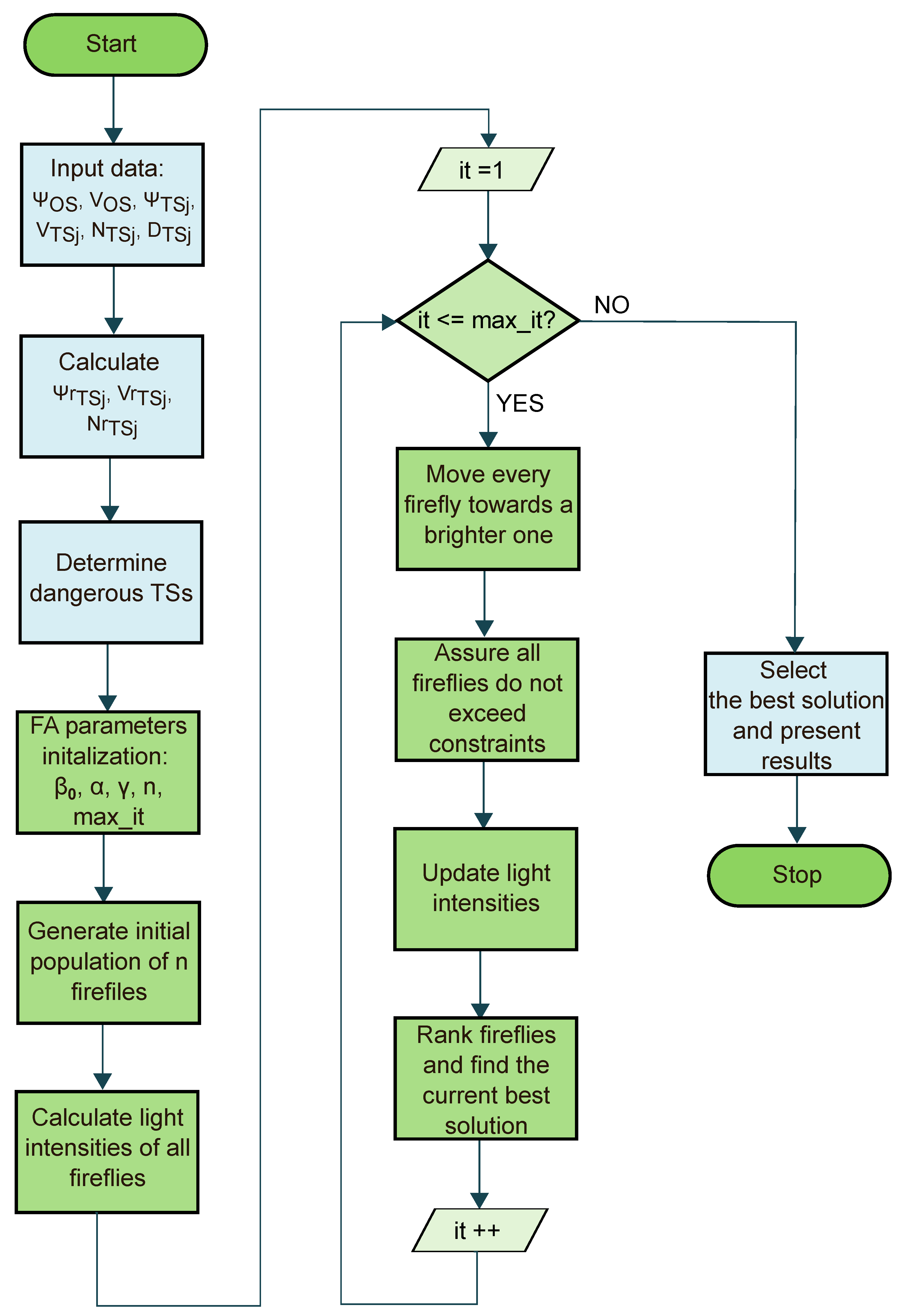
The rest of the paper is organized as follows. Section 2 compares the computational intelligence methods for ship collision avoidance presented in the recent literature, stating their most important advantages and limitations. Section 3 introduces two of the swarm intelligence methods, the Ant Colony Optimization and the Firefly Algorithm, applied for safe trajectory planning in a collision situation at sea. The inspiration for the development of these approaches, operation principle of the methods, flowcharts of the algorithms with explanations and applied assumptions are given in this section. Section 4 describes the carried-out simulation test and presents examples of the obtained results. In Section 5, both the ACO and FA approaches are compared and their most important features and differences are underlined. The research is summarized in Section 6.

2. Related Works

This section presents the results of a comparative analysis of the most recent approaches based on the computational intelligence applied in the collision avoidance systems.

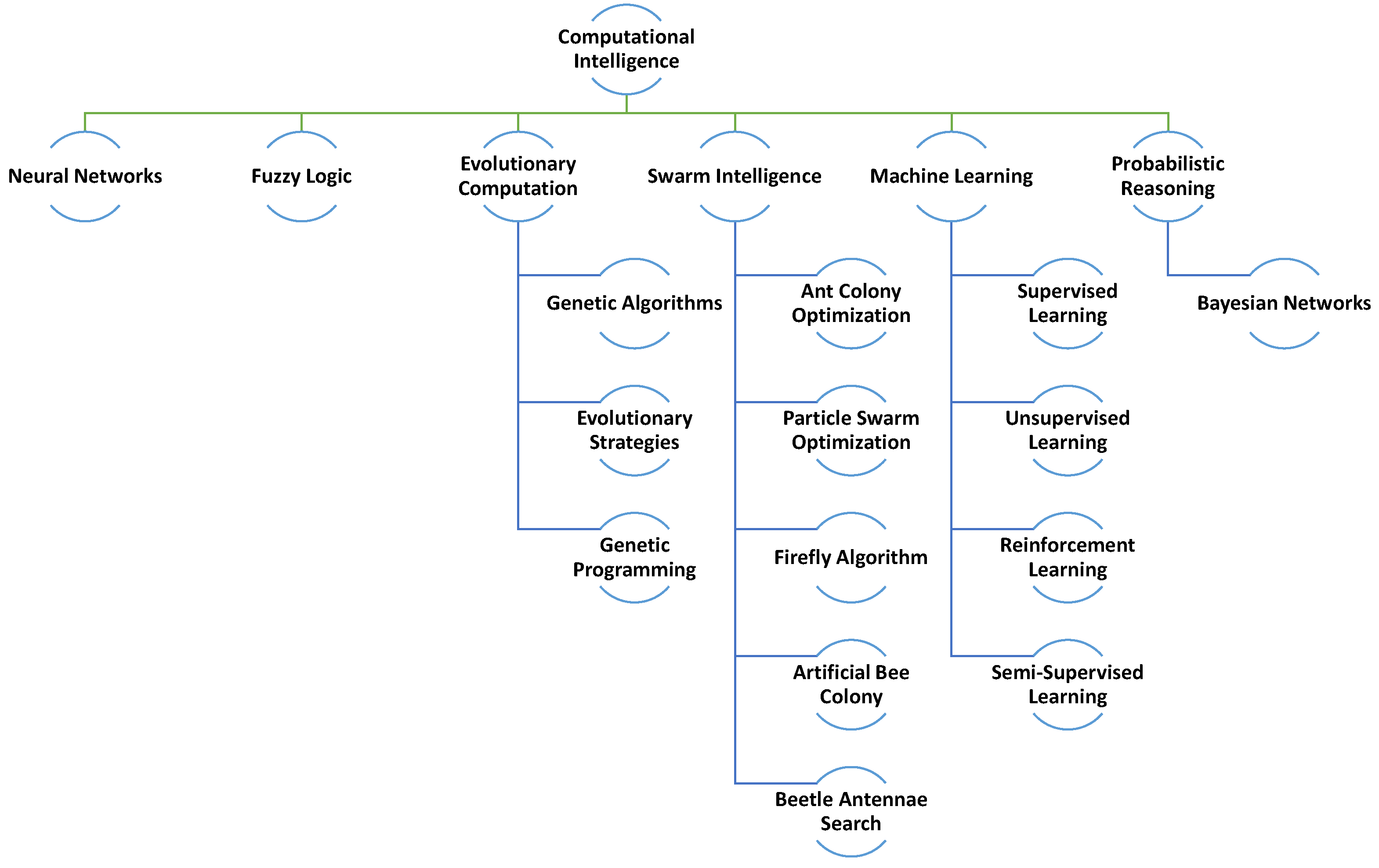
Computational intelligence (CI) methods are a subgroup of artificial intelligence (AI) approaches concentrated on the development of decision-making systems for complex problems, e.g., in changing environments. Methods classified to this group include the following: Neural Networks (NNs); Fuzzy Logic (FL); Evolutionary Computation (EC), such as genetic algorithms, evolutionary strategies and genetic programming; Swarm Intelligence (SI), such as Ant Colony Optimization (ACO) or particle swarm optimization (PSO); Machine Learning (ML), including supervised learning, unsupervised learning and reinforcement learning; and Probabilistic Reasoning (PR), such as Bayesian networks. These methods are applied for solving various real-world problems, e.g., in robotics, financial forecasting or control systems. Figure 1 presents the classification of the most common computational intelligence methods.

Figure 1. The classification of the most common computational intelligence methods. Source: author’s own.

The compared methods are presented in Table 1. The algorithms proposed in the recent literature were compared in terms of the following features:

• The applied computational intelligence method;
• The year of the paper publication;
• The International Regulations for Preventing Collisions at Sea (COLREGs) consideration [1];
• The consideration of static obstacles;
• The maximum number of dynamic obstacles (target ships) taken into account;
• The verification method—simulations and/or real experiments.

Table 1. A comparative analysis of the recent computational intelligence methods for ship collision avoidance.

Method	Year	COLREGs	Static Obstacles	Dynamic Obstacles	Simulations/Real exp.
DRL [2]	2023	yes	yes	up to 5	sim.
ANN [3]	2023	yes	no	1 TS	sim.
APF-ACO [4]	2023	yes	yes	up to 3	sim.
DRL [5]	2021	yes	no	up to 10	sim.
DRL [6]	2021	yes	no	up to 5	sim.
DRL-APF  [7]	2021	yes	yes	up to 4	sim.
IRL [8]	2020	yes	no	1 TS	sim.
DRL [9]	2020	yes	no	up to 3	sim./exp.
BAS [10]	2019	yes	no	up to 2	sim.
MARL [11]	2022	yes	no	up to 4	sim.
DRL [12]	2019	no	yes	1 TS	sim.
DRL [13]	2019	yes	no	up to 3	sim./exp.
I-Q-BSAS [14]	2019	yes	no	up to 4	sim.
FL [15]	2019	yes	no	up to 3	sim.

Table 1. A comparative analysis of the recent computational intelligence methods for ship collision avoidance.

Method	Year	COLREGs	Static Obstacles	Dynamic Obstacles	Simulations/Real exp.
DRL [2]	2023	yes	yes	up to 5	sim.
ANN [3]	2023	yes	no	1 TS	sim.
APF-ACO [4]	2023	yes	yes	up to 3	sim.
DRL [5]	2021	yes	no	up to 10	sim.
DRL [6]	2021	yes	no	up to 5	sim.
DRL-APF  [7]	2021	yes	yes	up to 4	sim.
IRL [8]	2020	yes	no	1 TS	sim.
DRL [9]	2020	yes	no	up to 3	sim./exp.
BAS [10]	2019	yes	no	up to 2	sim.
MARL [11]	2022	yes	no	up to 4	sim.
DRL [12]	2019	no	yes	1 TS	sim.
DRL [13]	2019	yes	no	up to 3	sim./exp.
I-Q-BSAS [14]	2019	yes	no	up to 4	sim.
FL [15]	2019	yes	no	up to 3	sim.

The analysis of the results from Table 1 allows us to note that, recently, machine learning approaches were most commonly applied for solving the ship collision avoidance problem. Among ML methods, deep reinforcement learning (DRL) was applied most often.

In [2], the authors proposed a decision-making model for solving the collision situation at sea based on the Partially Observable Markov Decision Process (POMDP). The authors stated that the advantages of this approach are the efficiency of addressing the environment’s complexity and uncertainty, and the improved decision accuracy. The convolutional neural network (CNN) was applied in order to extract the features of the images used for the state observation. The model training was performed with the use of the Proximal Policy Optimization (PPO) algorithm. Finally, the route guidance method, called the PPO for POMDP with guidelines under dense reward (G-IPOMDPPPO), was introduced by the authors in this research. The COLREGs consideration was included in the research. It was assumed that an agent selects the decision-making action according to the rules defined for different encounter situations, e.g., a head on situation, a crossing situation, an overtaking situation and a static obstacles situation. The results included situations with a few static obstacles, modeled as black rectangles, and up to five dynamic obstacles (target ships). The authors stated that the proposed image-state observation allowed for solving the problem of incomplete information and partial observability in collision avoidance situations. They also formulated some further research directions, such as the inclusion of the ship dynamics and the environmental characteristics in their model and a method of tackling the unpredictable behavior of target ships.

An another DRL-based approach was proposed in [5]. In this research, similarly as in [2], the actor–critic DRL algorithm called proximal policy optimization (PPO) was applied. It was used for the calculation of a collision avoidance path for the most dangerous target ship. An asymmetric ship domain was proposed in order to obtain a COLREGs compliant path. The introduced method was tested in simulations with up to 10 target ships and compared with the A* algorithm. The authors stated that their method proved high learning performance and stable learning convergence. The authors proposed considering static obstacles based on data from the Electronic Navigational Charts (ENC) in their future works and including the consideration of the COLREGs rule 9, related to navigation in the narrow channels.

In [6], the authors also applied the proximal policy optimization algorithm (PPO). They used the idea of the obstacle zone by target (OZT) for the collision risk assessment. The structure of the network applied in the PPO included long short-term memory (LSTM), a type of recurrent neural network (RNN). The authors used two types of control methods for training the model in the continuous action spaces. The first one was the rudder control model. The output of this approach was the rudder angle. The second one was the autopilot model. The output of this method was the heading angle. In order to receive a solution compliant with the COLREGs, a small positive reward was applied for the starboard side maneuvers. The navigation environment considered in this research did not include static obstacles such as coast lines or buoys. The results presented in the paper included situations with up to five target ships. In future works, the authors planned to develop a model with better course stability that would also be able to deal with changes in the motion parameters of target ships.

A different solution, but also based on DRL, was proposed in [9]. An encounter situation, fed into the DRL algorithm as input data, was represented using a grid map. The grid map included information on the target path, as well as the dynamic and static obstacles. The developed DRL network, based on dual DQN and double DQN structures, could select one of three behaviors such as path following, starboard side avoidance and port-side avoidance, depending on the considered encountered situation. The method was verified in simulations as well as in real experiments with the use of the WAM-V unmanned surface vehicle (USV) platform with up to three target ships. In future works, the authors planned to extend the action space to ship’s speed control.

In [12], the authors also proposed a DRL-based approach for intelligent decision-making in a collision situation at sea. The model was based on the deep Q-learning approach. Long short-term memory (LSTM) was used as the deep neural network. The navigation environment was modeled as a grid map. The COLREGs were not considered in this research. The method was implemented in the MATLAB environment. A simulation test with nine static obstacles, modeled as polygons, and with one dynamic obstacle was presented in the paper. The authors stated that their algorithm has a strong self-learning ability, as it performs adaptive avoidance in an unknown environment through online learning. In future research, they planned to test the model in more complex unknown environments, investigating water depth input and ocean currents disturbances.

Deep Q-learning was also proposed in [13] for solving the ship collision avoidance problem. The introduced model considered ship maneuverability, the human experience and the COLREGs. The human experience included, among other things, the ship domain and the predicted area of danger (PAD). The model was verified in simulations and real experiments with ship models. The results with three ships were presented in the paper. The authors stated that the numerical results they obtained were mostly comparable to the experimental results. For the further works, the authors proposed the consideration of the speed changes as actions in the collision avoidance process.

A method combining the DRL and the artificial potential field was proposed in [7]. The deep Q-learning network (DQN) was applied as the DRL algorithm. The artificial potential field (APF) algorithm was used for the improvement of the action space and the reward function of the DQN algorithm. A mechanism enforcing the COLREGs compliance of the solution was also implemented in this research. The COLREGs actions were included in the collision avoidance reward function. The method was tested in simulations with static and up to four dynamic obstacles. It was also compared with the DQN, DDPG, RRT, A* and APF algorithms in situations with static obstacles. The results confirmed that the proposed algorithm calculates collision avoidance actions conforming to COLREGs. The authors planned to consider environmental factors in their future works and to combine the proposed approach with a model-based DRL algorithm.

In [8], the inverse reinforcement learning (IRL) method was proposed for obtaining the optimal policy from the expert’s demonstrations. The method was verified in simulations, regarding simple encounter situations with one target ship, covered in COLREGs, such as head-on, crossing and overtaking. The presented results proved that the learned policy had similar performance with the expert demonstrations. In their future works, the authors planned to collect the real navigation data and include them in the developed approach.

In [11], the multi-agent reinforcement learning (MARL) algorithm, compliant with COLREGs, was applied for multi-ship collision avoidance. In this approach, every ship taking part in the considered collision situation was regarded as an agent. The algorithm calculated safe paths for all of the ships. The COLREGs were included in the reward function, similarly as in other RL-based approaches. The method was verified in simulations with up to four ships. In future works, the authors planned to implement a more accurate maneuverability model, optimization of the collision-free paths and comparative tests with other similar methods.

The application of Bayesian regularized artificial neural networks (BRANNs) for collision avoidance in the open sea was presented in [3]. The neural network was applied for determining the proper time and sufficient collision avoidance actions. The developed controller was verified with the use of a ship-handling simulator in test cases with one target ship. The authors stated that their approach was limited to cases such as overtaking a ship in front, which is to be corrected in their future works.

The application of fuzzy logic combined with a neural network for ship collision avoidance was proposed in [15]. The approach was compared with a method based on game theory. Both algorithms were implemented in the MATLAB programming language and verified using test cases with up to three target ships. In future works, the authors planned to perform sensitivity analyses of safe ship control, considering the changes in the process model parameters and the inaccuracy of information from the radar system.

The second largest subgroup of computational intelligence methods presented in the recent literature and applied to the ship collision avoidance problem was swarm intelligence. A hybrid method, combining the use of the APF and Ant Colony Optimization (ACO), was proposed in [4]. The developed algorithm was tested in simulations with both static and dynamic obstacles. The results of test cases with up to three target ships were presented in the paper. The method considered the COLREGs. The authors stated that they applied the ACO in order to solve the problem of local optimality of the solution, which they observed using only the APF method.

In [10], the authors introduced the application of the model predictive control and an improved beetle antenna search (BAS) algorithm for ship collision avoidance. The approach was verified with the use of simple encounter scenarios with up to two target ships, defined in COLREGs, such as head-on, crossing and overtaking. In their further works, the authors of this paper planned to carry out the sensitivity analysis of the simplified model parameters under different speeds in order to extract the parameters sensitive to speed changes. They also suggested the need for the use of different prediction horizons to achieve fine-tuning of the method.

In [14], a hybrid method based on model predictive control (MPC), an improved Q-learning beetle swarm antenna search (I-Q-BSAS) algorithm and neural networks was proposed for solving multi-ship encounter situations. The method was validated by simulation tests with up to four target ships. The presented method used the weighting approach for considering both the safety and the economy factors in the ship collision avoidance. The authors planned to apply a multi-objective Q-BSAS algorithm in their future research.

Analysis of the computational-intelligence-based collision avoidance methods for ships introduced in the recent literature allowed us to formulate the following summarizing remarks:

• In recent years (2019–2023), most of the developed approaches utilized different DRL methods;
• The second most-represented subgroup of approaches were methods based on swarm intelligence;
• Most of the proposed methods considered COLREGs;
• Most of the presented approaches did not consider static obstacles;
• Most of the algorithms were verified in simulations—real experiments were performed very rarely;
• A few (up to five) target ships were considered in most of the simulation tests.

The similar problems of collision avoidance and safe path planning also relate to other types of vehicles and moving objects, e.g., unmanned underwater vehicles (UUVs). Recent approaches for UUVs were proposed in [16], where a deep reinforcement learning algorithm was proposed for solving this task, and in [17], where the ant colony algorithm was applied. An algorithm based on reinforcement learning for unmanned aerial vehicles (UAVs) was proposed in [18]. A hybrid method, combining the neuro-fuzzy and modified grasshopper optimization algorithm (NFMGOA), was introduced in [19] for path following and collision avoidance of UAVs. These are just a few examples of recent works in the domains of UUVs and UAVs. Many more approaches can be found in the field of mobile robots, where machine learning methods also constitute a leading group. In [20,21], the authors applied reinforcement learning, and in [22], the Adaptive Stochastic Gradient Descent Linear Regression (ASGDLR) algorithm was proposed for collision avoidance and path planning of a mobile robot.

3. Swarm Intelligence for Ship Collision Avoidance

This paper is aimed at the detailed comparative analysis of two swarm intelligence methods applied for solving the ship collision avoidance problem: the Ant Colony Optimization (ACO)-based algorithm and the Firefly Algorithm (FA). This section introduces the applied concepts.

Swarm Intelligence is a group of approaches inspired by the collective behavior of social animals, such as ants, bees, fish and birds, as shown in Figure 2. The features observed in these living organisms, such as self-organization, flexibility and robustness, inspired researchers to develop mathematical descriptions of their behavior, which are now applied in many areas of science and industry. They are commonly applied for optimization and distributed problem-solving.

Figure 2. Swarms in nature: bee colony (left side); bird flock (right side). Source: Available online at https://www.pexels.com, accessed on 4 January 2024.

3.1. Ant Colony Optimization for Safe Trajectory Planning

3.1.1. Ant Colony Optimization Background

Ant Colony Optimization is an algorithm inspired by the foraging behavior of ants (Figure 3). It was first applied by Marco Dorigo in the early 1990s for solving the Traveling Salesmen Problem (TSP) [23].

Figure 3. Insects being inspiration for the development of SI algorithms: ants (left side); a firefly (right side). Source: Available online at https://www.pexels.com, accessed on 4 January 2024.

The TSP is a combinatorial optimization problem. The objective of this issue is to find the shortest route between a number of cities starting from a predefined city and returning to that city, with the assumption that every city can be visited only once. This is an NP-hard problem, what means that there does not exist an algorithm that allows solving all instances of the problem optimally in a polynomial time. The TSP is commonly used as a benchmark problem for the evaluation of the developed algorithm’s performance and comparison with other methods and their results [24].

The ACO concept was developed as a result of the observation of the ant colony behavior in the task of moving between the nest and a food source. These observations led to the conclusions that the ants exhibit some special mechanisms in their foraging behavior that enable, over time, finding the shortest path between the food source and their nest. It was found that they use some special indirect communication mechanism by leaving pheromone trails on the ground and sensing them afterwards. Other ants, when exploring the surroundings, decide to use a path where the pheromone trail concentration is higher.

3.1.2. Ant Colony Optimization Operation Principle

In the Ant Colony Optimization algorithm, after parameters initialization, a population of artificial ants start to construct solutions. Every ant constructs its solution (a candidate path) by using an action choice rule. This probabilistic method considers the pheromone trail amounts deposited on the possible solution components (parts of the ants’ paths) and heuristic information, called visibility. When all of the ants in the current iteration finish constructing their paths, the pheromone trail amount on the possible solution components (parts of the ants’ paths) is updated. This stage is composed of pheromone evaporation and pheromone deposit. The solution construction and the pheromone trail update procedures continue until the termination criterion is met, which can be a maximum number of iterations.

3.1.3. Ant Colony Optimization for Ship Collision Avoidance

An algorithm applied for solving the ship collision avoidance problem has to fulfill a number of assumptions and constraints, such as the following:

• The solution should conform to the International Regulations for Preventing Collisions at Sea (COLREGs) [1];
• The calculated path should allow for a safe passage of a ship between the current ship’s position and a defined final position, e.g., the next waypoint of the ship’s global path;
• The scope of input data for the collision avoidance algorithm, describing the current situation at sea, should be stated;
• The way of taking static (lands, shallows) and dynamic obstacles (target ships) into account should be defined, e.g., restrictions modeling as convex and concave polygons, ship domains around target ships’ positions;
• The optimization criterion should be defined, e.g., minimal path length, minimal and maximal course changes, minimal transition time, etc.;
• The applied motion model of all ships considered in the collision situation being solved should be defined, and whether it is assumed that target ships maintain their motion parameters during problem solving;
• The maximum acceptable run time of the algorithm, which will assure the solution’s applicability in practical applications, should also be defined.

Some of the initial and final stages of a collision avoidance algorithm for ships might be identical, regardless of the optimization method applied. Figure 4 and Figure 5 present flowcharts of the Swarm Intelligence algorithms compared in this paper: ACO and FA. As it can be noticed in these figures, the common parts of both algorithms have been marked in blue color. These are input data reception, calculation of relative courses, speeds and bearings of the target ships, determination of dangerous target ships, posing the collision risk and selection of the final best solution, and the graphical and numerical presentation of results. The other parts of the algorithms, responsible for the calculation of a safe path for a ship, are specific and dependent on the applied optimization method, ACO or FA.

Figure 4. A flowchart of the Ant Colony Optimization algorithm for ship collision avoidance. Source: author’s own.

Figure 5. A flowchart of the Firefly Algorithm for ship collision avoidance. Source: author’s own.

Target ships whose courses intersect with the course of their own ship and the intersection point of the trajectories of both vessels placed within the area of observation are regarded as dangerous target ships. For each of such objects, the distance of an own ship from the intersection point and the time after which an own ship will arrive at the intersection point is calculated by the algorithm.

Both algorithms apply the kinematic model of ships’ motion in the process of collision avoidance at sea, defined by the following equations:

$$\begin{array}{c}\hfill \dot{x_1}=V·cosu\left(t\right)=V·cos\Psi \left(t\right)\\ \hfill \dot{x_2}=V·sinu\left(t\right)=V·sin\Psi \left(t\right)\\ \hfill {\dot{x}}_{2·j+1}=V_j·cos{\Psi }_j\left(t\right)\\ \hfill {\dot{x}}_{2·j+2}=V_j·sin{\Psi }_j\left(t\right)\end{array}$$

(1)

where the state and control variables are $x_1=x$, $x_2=y$, $x_{2j+1}=x_j$, $x_{2j+2}=y_j$, u = $\Psi$ and j = 1, 2, …, m, where m is the number of target ships.

In the ACO-based algorithm, in the next stage, a construction graph composed of possible own ship turning points in the solution space is built. In this construction process, dynamic navigational constraints in the form of target ships’ domains are also considered. The own ship’s possible turning points placed inside the areas occupied by the target ships’ domains are removed from the construction graph.

Afterwards, ACO specific parameters are initialized, such as the initial value of pheromone trail ${\tau }_0$ on all vertices; $\alpha$ and $\beta$ coefficients, used in the formula for the probability of the ant’s next move; pheromone evaporation rate $\rho$ (0 < $\rho$ <= 1); number of artificial ants—n; maximum number of ant’s steps—$max\text{\_}steps$; and maximum number of iterations—$max\text{\_}it$.

The next two steps are repeated until the maximum number of iterations is reached. These are constructions of solutions by the artificial ants and pheromone trail update procedure.

$$P_{w{p}_{ij}}^{ant}\left(t\right)=\frac{{\left[{\tau }_{w{p}_j}\left(t\right)\right]}^{\alpha }·{\left[{\eta }_{w{p}_{ij}}\right]}^{\beta }}{{\sum }_{l\in w{p}_i^{ant}}{\left[{\tau }_{w{p}_l}\left(t\right)\right]}^{\alpha }·{\left[{\eta }_{w{p}_{il}}\right]}^{\beta }}$$

(2)

$${\tau }_{w{p}_j}(t+1)=(1-\rho )·{\tau }_{w{p}_j}\left(t\right)+\sum _{ant=1}^{ant\text{\_}number}\Delta {\tau }_{w{p}_j}^{ant}\left(t\right)$$

(3)

The construction of solutions by artificial ants is carried out in the following way:

• Each artificial ant starts building its path from an initial vertex $w{p}_0$ with coordinates ($x_0$, $y_0$), which is the current own ship’s position.
• After that, each ant builds its path until it reaches the end vertex $w{p}_0$ with coordinates ($x_e$, $y_e$) or it achieves a maximum number of steps—$max\text{\_}steps$.
• In every step, an ant uses the action choices rule to select the next vertex from neighboring vertices. Equation (2) is used for the calculation of the next vertex selection probability. The choice of the next vertex depends on the pheromone trail amount on vertex j adjacent to the current vertex i − ${\tau }_j\left(t\right)$ and a heuristic information ${\eta }_{ij}$. The ${\eta }_{ij}$ is calculated as an inverse of the distance between the current vertex i and the neighboring vertex j.
• When every ant in a given iteration finishes building its path, the pheromone trail update is carried out according to Equation (3). It is composed of two parts: the pheromone evaporation, which allows the ants to “forget” their bad decisions, and the pheromone deposit, the aim of which is to reinforce the good solutions. In this procedure, a certain amount of the pheromone trail is added to every vertex on the graph belonging to the paths built by the ants in a given iteration.

3.2. Firefly Algorithm for Safe Trajectory Planning

3.2.1. Firefly Algorithm Background

The Firefly Algorithm is inspired by the flashing behavior of fireflies. It was introduced by Xin-She Yang [25] in 2008. Fireflies are insects that use bioluminescence for communication and attracting mates (Figure 3). Bioluminescence is a mechanism of light production through a chemical reaction taking place in the fireflies’ bodies. The intensity of light emitted by the fireflies is variable. The brighter the firefly, the more attractive it is to other fireflies.

3.2.2. Firefly Algorithm Operation Principle

In the Firefly Algorithm, similarly as in other population-based methods, the first step is the generation of the initial population of fireflies, which represent candidate solutions for the considered optimization problem. Afterwards, the light intensity of every firefly is calculated. It is applied in order to indicate the quality of every candidate solution—its fitness to the problem being solved. The next stage is the process of the fireflies’ movement, which expresses the modification of candidate solutions in order to achieve better results. In this phase, the mechanism of the fireflies’ movement towards brighter insects, observed in nature, is applied. Every firefly changes its position, moving towards a brighter neighbor firefly. In order to apply an exploration mechanism, a randomization factor is also applied in the formula defining the firefly movement. The decrease in firefly attractiveness, dependent on the distance between fireflies, is also modeled. A light absorption coefficient is used for that purpose. The phase of the fireflies’ movement and evaluation of the candidate solutions is continued until the termination criterion is achieved, which might be a maximum number of iterations.

3.2.3. Firefly Algorithm for Ship Collision Avoidance

FA for ship collision avoidance, similarly to the ACO-based approach, begins with the reception of input data; calculation of the relative courses, speeds and bearings of target ships; and dangerous target ships determination. Afterwards, the FA-specific parameters are initialized, such as the attractiveness at distance r = 0 − ${\beta }_0$, a parameter introducing randomness—$\alpha$, the light absorption coefficient—$\gamma$, the number of fireflies—n and the maximum number of iterations—$max\text{\_}it$. Then, an initial population of n fireflies (candidate paths) is generated. Every candidate path consists of the same initial waypoint $w{p}_0$ (the current own ship’s position); the final waypoint $w{p}_e$ (defined final own ship’s position); and an intermediate waypoint, which is randomly added to every candidate path. In the next step, light intensities for all fireflies in the initial population are calculated.

$$\begin{array}{ccc}\hfill {\displaystyle x_i^{t+1}}\hfill & =& \hfill {\displaystyle x_i^t+{\beta }_0{e}^{-\gamma r_{ij}^2}(x_j^t-x_i^t)+\alpha (rand-0.5)}\hfill \end{array}$$

(4)

$$\begin{array}{ccc}\hfill {\displaystyle r_{ij}}\hfill & =& \hfill {\displaystyle \sqrt{{(x_i-x_j)}^2+{(y_i-y_j)}^2}}\hfill \end{array}$$

(5)

After that, the following steps are repeated until the maximum number of iterations is achieved:

• Equation (4) is applied to calculate the movement of a firefly towards a brighter firefly.
• Verification of whether every firefly is placed within the solution space and does not exceed constraints (does not cause a collision with any of the target ships).
• Light intensities of new solutions (fireflies) are calculated.
• Fireflies are ranked according to their light intensities, and the current best solution (safe own ship’s path) is calculated.

As mentioned above, Equation (4) defines the movement of a firefly towards a brighter one, where $x_i^{t+1}$ is the new position of a firefly i at time $t+1$, $x_i^t$ is the actual position of a firefly i at time t, $x_j^t$ is the actual position of a firefly j at time t, ${\beta }_0$ is the attractiveness at distance r = 0, $\alpha$ is a parameter introducing randomness, $rand$ is a random number generator uniformly distributed in the range [0, 1], $r_{ij}$ is the distance between fireflies i and j, and $\gamma$ is the light absorption coefficient. The Euclidean distance between fireflies i and j ($r_{ij}$), influencing the rate of a firefly’s movement towards a brighter firefly, is calculated with the use of Equation (5).

4. Simulation Results

This section presents four test cases selected in order to verify the algorithms’ performance and their problem-solving capability. Both described Swarm-Intelligence-based collision avoidance algorithms were implemented in the Matlab programming language. The algorithms’ specific parameters used in calculations, listed in Table 2, were selected experimentally in order to achieve the best results in terms of both solution optimality and run time.

Table 2. ACO and FA parameters used in the simulation tests.

Algorithm	Parameters
ACO	$\alpha$ = 1, $\beta$ = 2, $\rho$ = 0.1, ${\tau }_0$ = 1, n = 10, $max\text{\_}it$ = 20
FA	${\beta }_0$ = 1, $\alpha$ = 0.4, $\gamma$ = 1, n = 20, $max\text{\_}it$ = 30

A hexagon-shape domain was applied around TSs with the following dimensions: the distance towards bow—1.05 NM, the distance of amidships—0.65 NM, the distance towards starboard side—0.65 NM, the distance towards stern—0.4 NM and the distance towards port side—0.4 NM.

Other shapes (and sizes) of the TSs domains, e.g., a circle or an ellipse, are also possible to be applied. However, it is recommended that the shape and size of the ship domain be selected in a way enforcing the COLREGs compliance of the calculated safe paths. Therefore, the starboard side should be larger than the port side and the distance towards the bow should also be larger than the distance towards the stern.

It is assumed that during the calculation process TSs maintain their motion parameters (the course and the speed). This assumption is common in the applications of collision avoidance algorithms for ships. It is assumed that the algorithm should return the solution in at most a few seconds and retrieve new input data concerning the position and motion parameters of TSs from the navigational equipment in order to recalculate the solution, if the change in the TSs parameters has been detected.

Table 3, Table 4, Table 5 and Table 6 present input data of all test cases, such as the course (${\Psi }_{OS}$) and the speed of an own ship ($V_{OS}$); the target ships’ courses (${\Psi }_{T{S}_j}$), speeds ($V_{T{S}_j}$) and bearings ($N_{T{S}_j}$); and distances of target ships from an own ship ($D_{T{S}_j}$). Table 7 shows the results obtained with the use of both ACO-based and FA-based algorithms, such as the safe path length in nautical miles, an own ship’s course at consecutive stages of the vessel’s movement along the safe path in degrees and the run time of algorithms in seconds. In order to evaluate the run time of the algorithms, the calculations for every test case were carried out 100 times and the worst, the best and the average run times were determined.

Table 3. Input data of test case 1 with 1 TS.

Ship	Ψ [°]	V [kn]	N [°]	D [NM]
$OS$	0	12	-	-
$T{S}_1$	180	10	0	7

Table 4. Input data of test case 2 with 1 TS.

Ship	Ψ [°]	V [kn]	N [°]	D [NM]
$OS$	0	12	-	-
$T{S}_1$	270	12	45	7

Table 5. Input data of test case 3 with 3 TSs.

Ship	Ψ [°]	V [kn]	N [°]	D [NM]
$OS$	0	12	-	-
$T{S}_1$	90	10	326	8.8
$T{S}_2$	180	12.3	6	14.3
$T{S}_3$	200	11.5	11	7.5

Table 6. Input data of test case 4 with 5 TSs.

Ship	Ψ [°]	V [kn]	N [°]	D [NM]
$OS$	0	20	-	-
$T{S}_1$	90	10.5	326	8.8
$T{S}_2$	180	12.2	355	7.3
$T{S}_3$	200	18	11	7.5
$T{S}_4$	270	7.3	27	6.8
$T{S}_5$	275	15.7	35	6

Table 7. Output data of all test cases.

Test Case	Algorithm	Path Length [NM]	Ψ [°]	The Best Run Time [s]	The Worst Run Time [s]	Average Run Time [s]
1	ACO	9.48	45, 353	4.6644	9.9772	5.9082
1	FA	9.18	13, 350	0.7077	0.8036	0.7191
2	ACO	9.22	11, 346	5.1187	17.092	9.3779
2	FA	9.19	9, 345	0.4181	0.5324	0.4395
3	ACO	9.22	11, 346	5.1874	12.3709	7.1892
3	FA	9.31	15, 346	0.4271	0.5549	0.4435
4	ACO	9.93	18, 326	5.8507	22.5903	11.6635
4	FA	9.68	20, 337	0.9477	1.1061	0.9654

The OS initial course is assumed to be 0 degrees. The course values in Table 7 show the calculated OS course at consecutive stages of the vessel movement along the determined path. For example, for test case 1 using ACO, it means that the ship should perform a maneuver to the starboard side, changing the course from 0 degrees to 45 degrees. Afterwards (when the vessel has achieved waypoint 1), in order to return to the defined final waypoint, the ship should perform a maneuver to the port side by changing the course by 52 degrees, from 45 degrees to 353 degrees (353 is the course the vessel should keep in order to return to the final waypoint).

Both algorithms are constructed in a way that allows for the achievement of the same solution for every run of calculations with the same input data, which is very important for the practical application of such an approach. However, due to the probabilistic nature of both algorithms, the run time of the algorithm is variable. Therefore, the repetition of calculations (100 times) for every test case and the comparison of the run time of algorithms is important, as it allows to determine the best and the worst result in terms of the time needed by the algorithm to return a solution.

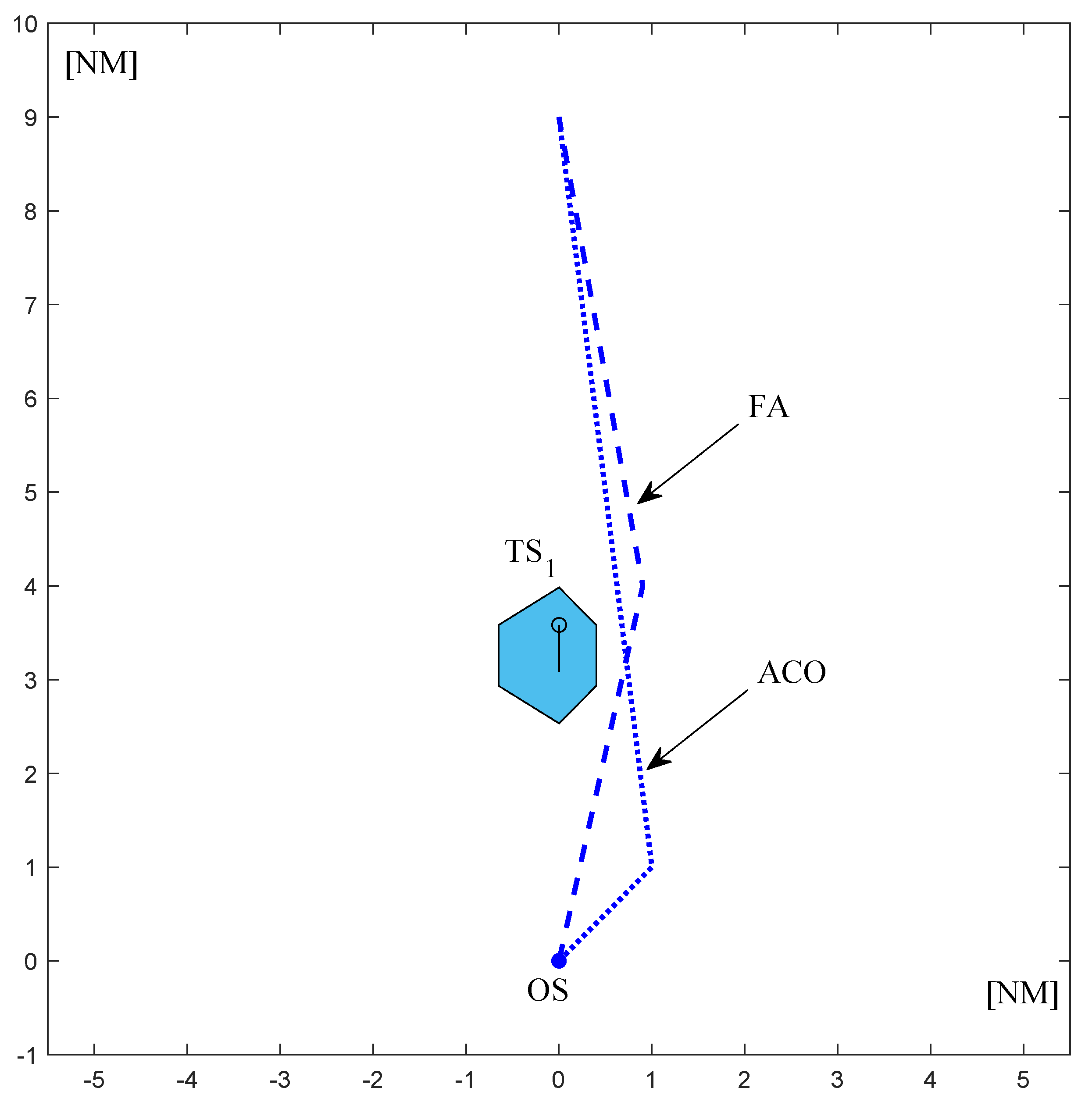
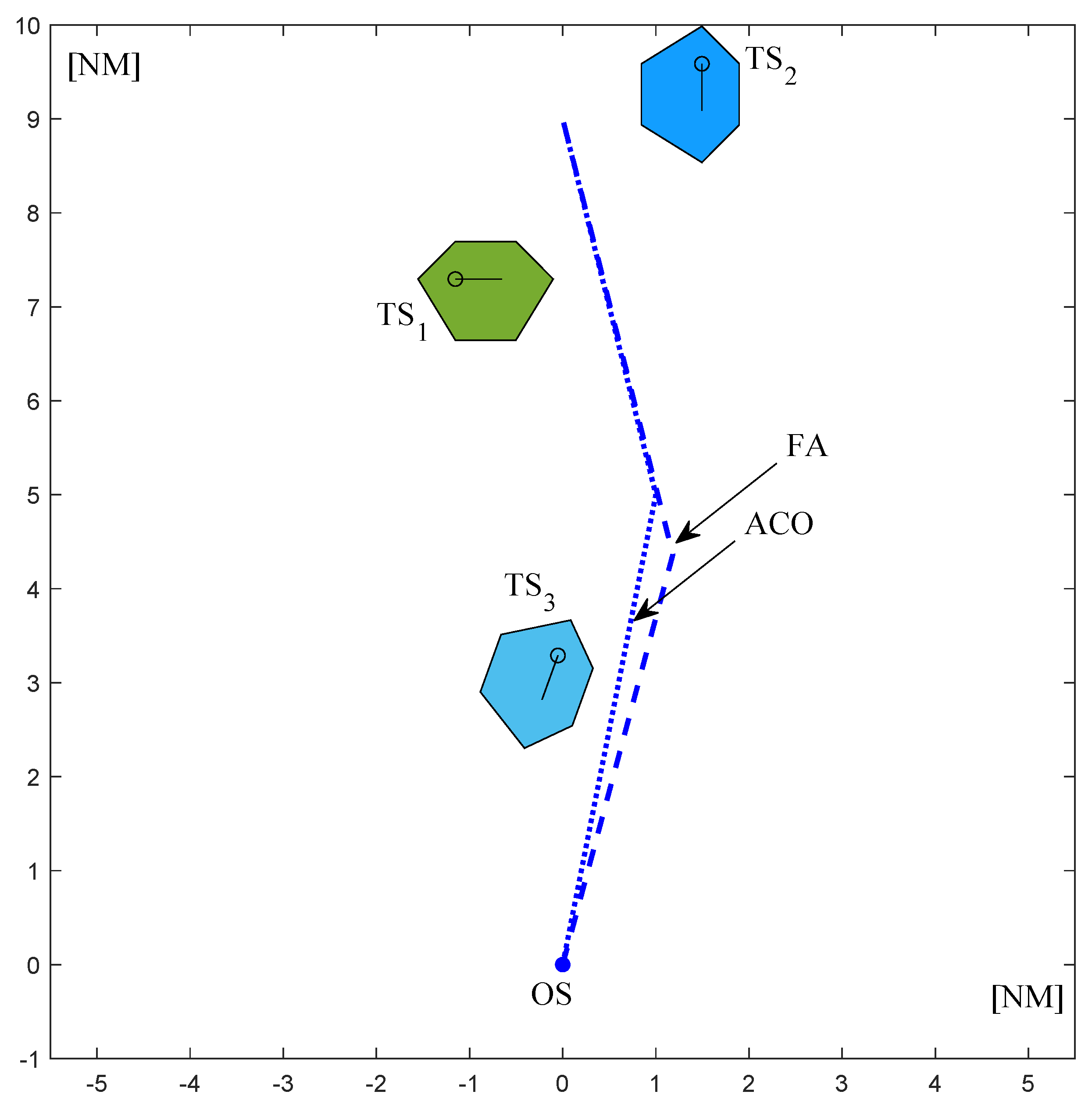
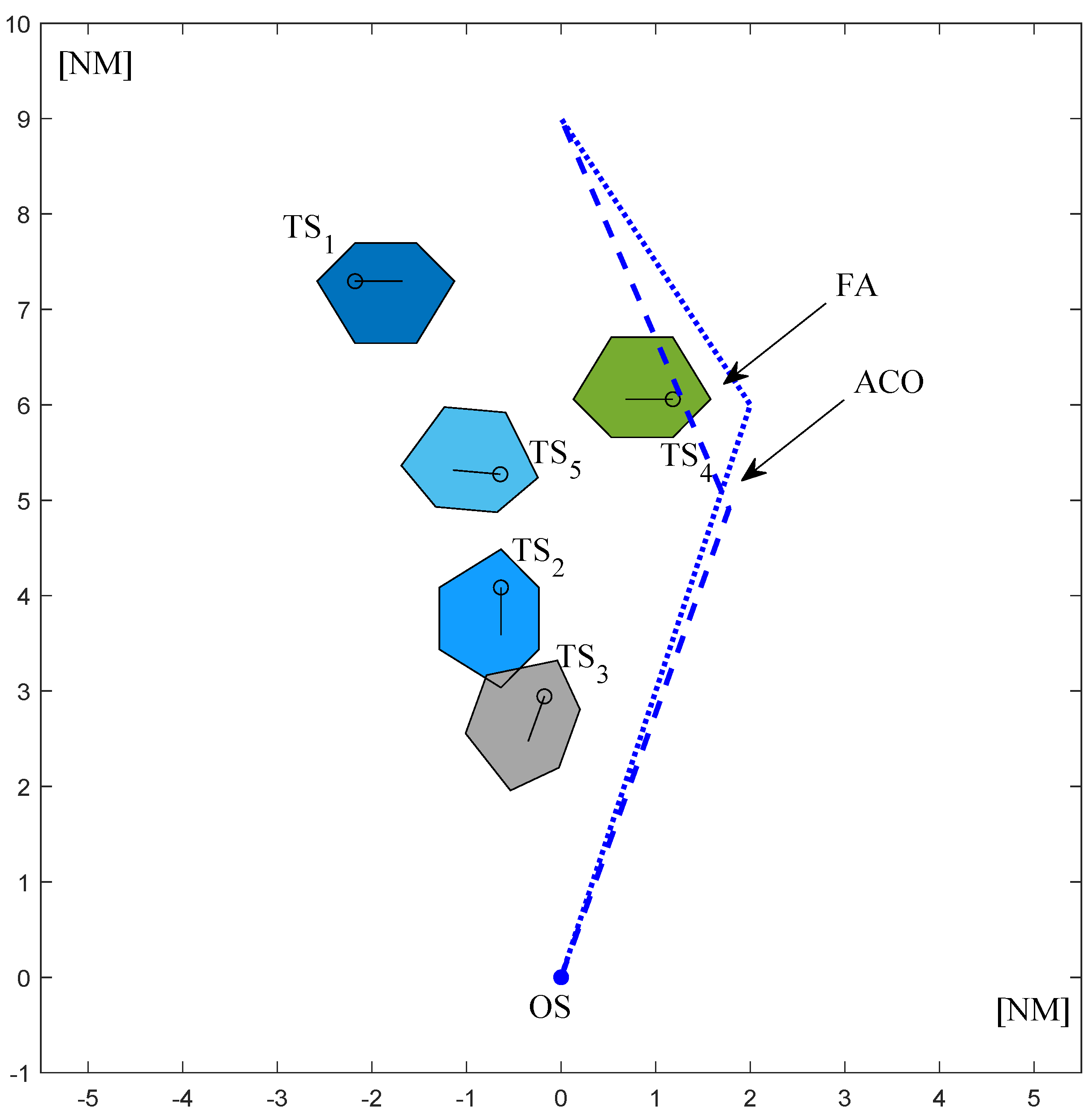
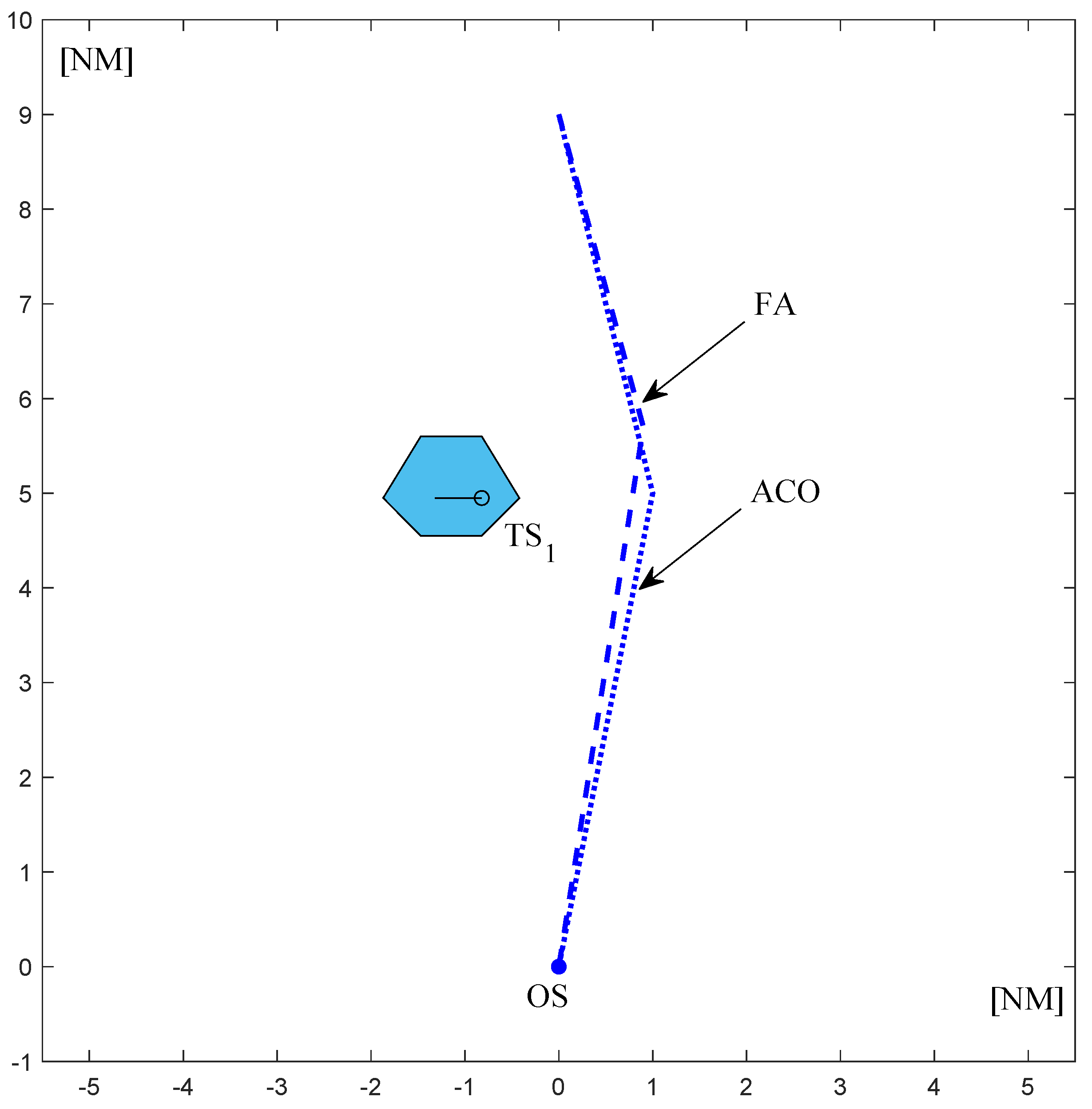
Figure 6, Figure 7, Figure 8 and Figure 9 present graphical solutions determined by the ACO-based and FA-based collision avoidance algorithms for tested scenarios. Both algorithms verify the calculated solution before the presentation of results in a way very similar to the trial maneuver function of the ARPA system, where the OS and the TSs are placed at consecutive positions resulting from their motion parameters (courses and speeds) and the algorithm verifies whether the ships do not collide with each other in any of these positions.

Figure 6. A comparison of own ship’s trajectories for test case 1 calculated by FA and ACO. Source: author’s own.

Figure 7. A comparison of own ship’s trajectories for test case 2 calculated by FA and ACO. Source: author’s own.

Figure 8. A comparison of own ship’s trajectories for test case 3 calculated by FA and ACO. Source: author’s own.

Figure 9. A comparison of own ship’s trajectories for test case 4 calculated by FA and ACO. Source: author’s own.

5. Discussion

Two swarm intelligence approaches were applied for ship collision avoidance and compared. The results of this comparative analysis are presented in Table 8. The differences are highlighted in gray color.

Table 8. A comparative analysis of ACO and FA applied for ship collision avoidance.

Feature	ACO	FA
solution construction	artificial ants movement on the construction graph	modification of the population of fireflies
optimization criterion	path length	path length
constraints consideration	TS domain	TS domain
constraints violation	an ant finds a solution not exceeding constraints	candidate solution corrected during solution construction
COLREGs enforcement	shape and size of TS domain	shape and size of TS domain
safe path optimization	trajectory optimization algorithm further applied	no further optimization
termination condition	maximum number of iterations	maximum number of iterations
solution efficiency	for 1 out of 4 presented test cases, shorter path was achieved	for 3 out of 4 presented test cases, shorter path was achieved
run time	several seconds	up to a second

For both algorithms, the best solution is the shortest path, which is a common optimization criterion used in path planning. Both algorithms consider target ships using the target ship domain. The COLREGs fulfillment is enforced by a proper shape and size of a ship domain, and the termination condition is the maximum number of iterations in both algorithms.

The constraints violation procedure is different in both algorithms. In ACO, artificial ants construct their paths not exceeding the constraints (instantaneous positions of target ships), but such a solution is further optimized by the trajectory optimization algorithm, removing unnecessary turning points. In FA, the candidate solution is corrected during the solution construction procedure, when the constraints’ violation has been detected.

The results of simulation tests confirmed that both algorithms return safe paths for all of the considered test cases. The determined own ship paths allow for the vessel’s movement between the initial position and the defined final position, without colliding with any of the target ships, assumed to be moving with constant motion parameters.

As it can be noticed in Table 7, the FA calculated shorter paths for 3 out of 4 considered test cases. The difference was equal to 0.3 nautical mile for test case 1, 0.03 nautical mile for test case 2 and 0.25 nautical mile for test case 4. For test case 3, the path determined by ACO was 0.09 nautical mile shorter.

In terms of the run time, the FA achieves significantly better results. Comparing the average run time for 100 calculations, for test case 1, the result of FA is over 9 s lower than that obtained by ACO. For test case 2, the difference is equal to over 16 s, for test case 3 it is almost 12 s, and for test case 4 it is over 21 s. What can also be noticed by analyzing the results is that the differences in the run time for different repetitions of calculations is much bigger for ACO than for FA. This results from the operation principle of the applied versions of algorithms. In the ACO, the solution construction procedure is based on the artificial ants’ movement on the construction graph. In FA, the construction of solutions is based on the modification of the population of fireflies, so the method of searching for the best solution is very different. Due to the operation principle, the ACO-based approach might be more effective for very complex encounter situations, where FA might have difficulties in finding a safe path.

Both algorithms return solutions compliant with COLREGs. The maneuvers are determined considering course changes as recommended by COLREGs—to the starboard side and large enough to be readily apparent for the other vessels.

The analysis of the obtained results allows for the following statements:

• Both algorithms are capable of calculating a safe, optimized path for an own ship in a collision situation at sea within an acceptable amount of time;
• The FA achieves better results than ACO in terms of the path length and the run time of the algorithm for most of the considered test cases;
• Both algorithms return solutions fulfilling COLREGs (especially rules 8b, 13, 14 and 15) [1];
• The ACO-based approach might be more effective for complex encounter situations;
• Both algorithms might constitute competitive approaches in relation to other recently introduced computational intelligence methods.

The limitations of both methods are as follows:

• The assumption that target ships do not change their motion parameters—if such a change is detected by navigational aids such as a radar with ARPA and/or AIS, the solution has to be recalculated for new input data;
• The lack of consideration of static obstacles, such as lands or shallows (possible to be implemented in the algorithms, but not included in the presented research);
• The lack of consideration of target ships dynamically changing heading angles and complex test cases demanding multiple maneuvers—such cases should be considered in future research in order to prove the robustness of these approaches;
• The variable run time for every run of calculations with the same input data and no guarantee of obtaining an optimal solution, but obtaining sub-optimal solutions within an acceptable time from the point of view of practical application of the method.

Future Trends and Challenges

A significant growth in the recent proposals for ship’s collision avoidance based on machine learning shows that this is the current trend and its continuation might be expected in the near future. However, swarm-intelligence-based and hybrid approaches also focus the attention of researchers working in this domain.

The autonomous navigation will primarily be developed for application to USVs and Maritime Autonomous Surface Ships, a ship plying on a short, fixed route between two ports, such as a ferry. The societal impact of autonomous shipping will include positive influence such as the possibility of the reduction of maritime accidents caused by human error. At the same time, accidents caused alongside the participation of advanced algorithms for navigation and vessel operation cannot be completely excluded. Therefore, the development of robust solutions, thoroughly tested before their final implementation, is of vital importance. The application of optimization algorithms to navigation and path planning can lead to the increased efficiency of maritime transport, as it may cause a reduction in fuel consumption. This will also have a positive environmental impact, as autonomous vessels in this way might reduce their greenhouse gas emissions and air pollution. The development of maritime shipping might cause a decrease in the demand for crew members but at the same time will create new jobs, e.g., in remote monitoring of autonomous ships.

6. Conclusions

The paper presented the application of two swarm intelligence optimization methods—Ant Colony Optimization and the Firefly Algorithm—applied for solving ship’s collision avoidance and path planning problems. Such methods can be applied in the Autonomous Navigation System (ANS) of unmanned and fully autonomous ships. The algorithms calculate a path composed of course change maneuvers between the current position of an own ship and a defined final position allowing for safe passing of encountered ships, called target ships. Both methods return repeatable solutions compliant with COLREGs in near-real-time, making them suitable for practical applications.

Future works should include consideration of both static obstacles, such as shallow waters, lands, buoys or military zones, and dynamic obstacles (target ships). Field experiments with ship models or smaller crafts, such as USVs, could constitute the next step towards the practical application of the proposed approaches.