TabNet: Locally Interpretable Estimation and Prediction for Advanced Proton Exchange Membrane Fuel Cell Health Management

Abstract

In the pursuit of advanced Predictive Health Management (PHM) for Proton Exchange Membrane Fuel Cells (PEMFCs), conventional data-driven models encounter considerable barriers due to data reconstruction resulting in poor data quality, and the complexity of models leading to insufficient interpretability. In addressing these challenges, this research introduces TabNet, a model aimed at augmenting predictive interpretability, and integrates it with an innovative data preprocessing technique to enhance the predictive performance of PEMFC health management. In traditional data processing approaches, reconstruction methods are employed on the original dataset, significantly reducing its size and consequently diminishing the accuracy of model predictions. To overcome this challenge, the Segmented Random Sampling Correction (SRSC) methodology proposed herein effectively eliminates noise from the original dataset whilst maintaining its effectiveness. Notably, as the majority of deep learning models operate as black boxes, it becomes challenging to identify the exact factors affecting the Remaining Useful Life (RUL) of PEMFCs, which is clearly disadvantageous for the health management of PEMFCs. Nonetheless, TabNet offers insights into the decision-making process for predicting the RUL of PEMFCs, for instance, identifying which experimental parameters significantly influence the prediction outcomes. Specifically, TabNet’s distinctive design employs sequential attention to choose features for reasoning at each decision-making step, not only enhancing the accuracy of RUL predictions in PEMFC but also offering interpretability of the results. Furthermore, this study utilized Gaussian augmentation techniques to boost the model’s generalization capability across varying operational conditions. Through pertinent case studies, the efficacy of this integrated framework, merging data processing with the TabNet architecture, was validated. This work not only evidences that the effective data processing and strategic deployment of TabNet can markedly elevate model performance but also, via a visual analysis of the parameters’ impact, provides crucial insights for the future health management of PEMFCs.

1. Introduction

The anticipated surge in energy consumption in the coming decades underscores the pressing need for renewable energy sources that significantly curtail carbon emissions. PEMFCs, a type of hydrogen fuel cells with a high efficiency, quick response time, and low operating temperature, have been increasingly deployed across a range of applications from industrial uses to portable electronics and as alternative power sources in transportation [1]. However, the longevity of PEMFCs is compromised by the degradation of critical components, a challenge that calls for sophisticated monitoring and predictive approaches.

In this context, PHM systems have been pivotal in assessing the degradation status of PEMFCs [2]. They harness historical and current operational data to estimate the time to failure and the likelihood of impending failure modes as per ISO 13381-1(2015) definitions [3]. Central to this prognostic process is the determination of an effective Health Indicator (HI), with the stack voltage commonly adopted as a reliable HI for its direct correlation with the cell’s health status [4].

Previous studies suggest that PHM techniques fall into three categories: hybrid, data-driven, and model-driven approaches, and prediction model selection is the central part of the prognostic. The prediction of the RUL through model-driven approaches primarily depends on the fuel cell’s loading conditions, material properties, and degradation and failure mechanisms [5]. However, the model-based method is complex, and it is challenging to establish degradation models for PEMFCs accurately. This is due to the fact that PEMFC degradation mechanisms operate on complex multi-time and multi-physical scales [6]. Moreover, the technique that relies on monitored historical data to anticipate the remaining lifespan of PEMFCs is the idea of a data-driven method. This approach is rapid and efficient since it does not require knowledge of fuel cell models or systems [7]. The model-driven and data-driven approaches are integrated into the hybrid method. The mathematical model describes the HI aging characteristics and uses an algorithm from a data-driven method to predict temporal data. Among these three methods, the data-driven method has been mostly studied and achieved remarkable results in recent research.

However, interpreting model decisions and results poses a challenge, as the internal decision-making process of these models is often opaque, requiring specialized software for transparency [8]. This highlights the importance of model interpretability, especially for regulatory or audit purposes, where a clear and repeatable method for deriving model decisions is crucial [9]. A pioneering data-driven model, long-short-term memory (LSTM) recurrent neural network (RNN), was proposed by [7] to solve the RUL prediction problem of PEMFCs. The raw data were reconstructed and filtered by using the locally weighted scatterplot grinding method. This method significantly reduced the data size and maintained the trend in sequential data. A characteristic of the LSTM model was that the target features could be fed as input to train the model. This characteristic improved the prediction performance and resulted in a highly satisfying output. Additionally, Wang et al. [10] suggested using differential evolution in combination with a stacked long-short-term memory (S-LSTM) model to forecast the RUL of PEMFCs. In [10], the data reconstruction and smoothing were not carried out, but ten features were selected as input. The S-LSTM stacks two LSTM models, and the optimal hyperparameters are obtained through the differential evolution. The experimental results show that S-LSTM achieved a 96% accuracy, which outperformed a model-driven method called particle filter and the random forest algorithm. Although the LSTM family achieves remarkable results, it is limited by its parallelism capability and requires significant computational resources.

Hence, other machine learning and deep learning methods have also been studied. For example, a unique method for predicting the degradation of PEMFCs combines the deep belief network (DBN) and the extreme learning machine (ELM) [11]. The DBN was utilized to derive high-quality degradation features from the raw data that contained uncertainty and nonlinearity. The ELM had excellent generalization capabilities that could reduce the possibility of overfitting and instability problems. The combination of DBN and ELM showed a high potential for degradation prediction under a static dataset. However, it was not tested on the more challenging dynamic dataset. Liu et al. [12] proposed a sparse autoencoder (SAE) and DNN-based technique targeting the dynamic operating condition. The experimental data were also reconstructed and smoothed using Gaussian weighted moving average filters. The SAE is employed to extract the predictive characteristics automatically, while a DNN is used for the RUL prediction. Three distinct training and test set configurations were used to validate the efficacy. According to the experimental results, the training set length of 500 h yielded the best prediction results for the approach.

Recently, some newly proposed deep learning models were utilized in the PEMFC RUL prediction problem. A novel transformer-based solution, proposed by Zhou et al. [13], applied a self-attention technique to identify the long-term dependencies in the data. In the data preprocessing stage, the input features of the model are manually selected after feature extraction and recombination. Then, they a specific embedding layer and a multi-layer transformer structure are incorporated. This model achieved a preliminary result on the real-world application dataset. However, it also had some limitations, such as high computational complexity and the requirement of large training data. The other method that combined transfer learning and the transformer model was introduced last year [14]. The core idea of this method is to first pre-train a transformer model on a static dataset and then transfer this model to the target dynamic dataset for fine-tuning. By using transfer learning, this method fully leverages the knowledge learned from the source dataset. The experimental results showed the model achieved over 80% prediction accuracy on the target dataset. The main advantage of this method was its strong generalization ability. On the contrary, a large amount of labeled data was needed to retrain the model. This might be unrealistic in many practical scenarios, as obtaining large amounts of labeled data is time-consuming and expensive.

In addition, Wang et al. [15] combined extreme gradient boosting (XGBoost) and TabNet to a provide better fitting performance in the photovoltaic (PV) prediction field. XGBoost helps select features automatically, and TabNet fits with the sequential data and forecasts the PV power. The model was applied to real-world PV data, and the results showed that TabNet could predict the fluctuation trend effectively.

The need for model clarity and interpretability makes black-box model predictions in XGBoost or traditional deep-learning models unattractive. However, TabNet provides feature significance and internal decision masks. The feature scores returned from TabNet indicate that explicitly selected features are essential for model decision-making and that there is no ambiguity in the model selection. Other features with high scores also differ from those with low scores. Adding decision masks provides more insights into the model’s decision-making process. The Attentive Transformer does not retain features that do not contribute to the model’s decision. The output of the decision masks captures this process. Access to these decisions is simple and does not require additional software packages. The ability of TabNet to quickly provide model interpretability can bridge this gap in deep learning as these attributes can provide enough model information to comply with regulatory requirements [16]. Overall, data-driven methods showcase the efficiency of leveraging historical data without the need for intricate fuel cell models. An appropriate data preprocessing technique is also helpful in obtaining a satisfactory result. Building upon the established need for robust PHM systems in enhancing the durability and reliability of PEMFCs, this paper intends to expand on the strengths of these data-driven techniques by integrating a new data preprocessing method with the TabNet algorithm. The contributions of this research are threefold, aiming to enhance the prognostic capabilities within the renewable energy sector:

• A new data preprocessing technique, Segmented Random Sampling Correction (SRSC), is introduced to enhance the treatment of continuous datasets by preserving their integrity and continuity while dynamically eliminating outliers based on segmented mean assessments.
• This study is the first to apply Gaussian augmentation exclusively to the prediction dataset, distinct from the training set. We emulate the natural variability present in real-world operational data by introducing slight perturbations via Gaussian noise during the prediction phase. This method bolsters the model’s generalization capabilities to unseen data, a critical step in ensuring robustness in predictive analytics.
• TabNet uses preprocessed data to identify key features in the PEMFC PHM system, with its feature scores emphasizing the importance of selected features in model decisions, enhancing model selection clarity. Decision masks enhance interpretability, offering insights into the model’s reasoning process. TabNet is a valuable tool for complex decision-making environments like PEMFC health management by improving transparency and confidence in model predictions.

The integration of TabNet into PHM systems represents a significant stride forward in the renewable energy domain, addressing the critical need for the predictive maintenance and prolonged operational viability of PEMFCs. The remaining parts of the paper are structured as follows: a review of the literature on the PHM system of PEMFCs is presented in Section 1. Section 2 describes the methodology of data preprocessing, the TabNet-based neural network structure, and the model evaluation metric; Section 3 presents the prediction result and the model performance applied to the experimental dataset; Section 4 concludes the achievements and discusses future works.

2. Methodology

2.1. Data Preprocessing

The data used in this article were sourced from the IEEE PHM 2014 Data Challenge quasi-dynamic dataset [17], comprising 25 variables and 127,372 data points. The effective preprocessing of time-series data is crucial for the precision of PHM systems in estimating the RUL of PEMFCs. We use SRSC to meticulously address noise and anomalies, safeguarding the authenticity of temporal patterns within the data.

During preprocessing, the dataset is initially segmented into multiple parts, each consisting of 1500 data points. Segmenting allows for a more nuanced approach to local data characteristics rather than applying a uniform treatment across the entire dataset. An average value, calculated within each segment, serves as a benchmark for determining upper and lower thresholds. However, instead of replacing an outlier with the average of neighbouring points, the SRSC method selects a random value from the preceding 100 data points. This random sampling strategy is designed to maintain the natural variability of the data, avoiding loss of trend information due to over-smoothing.

Moreover, a threshold percentage is set to identify outliers. If the value of a data point exceeds the range defined by the average of the segment plus or minus the threshold percentage, it is classified as an outlier. This strategy ensures that genuine data fluctuations are not mistaken for errors and that actual errors do not disrupt the analysis.

This approach mitigates data noise while preserving the actual dynamics of the dataset to the greatest extent possible. This is crucial for subsequent data analysis and modeling, as the data quality directly impacts the accuracy and reliability of the models. Applying this preprocessing method results in a cleaner and more representative dataset, facilitating the assessment and optimization of fuel cell performance. The replacement method, illustrated in Figure 1, maintains the inherent variance of the series, which is vital for further modeling and analysis.

Mathematically, the SRSC is represented as follows:

$$y_i=\left\{\begin{array}{cc}{x}_i,\hfill & \mathrm{if}L\le x_i\le U\hfill \\ x_{\mathrm{random}(i-\omega ,i)},\hfill & \mathrm{otherwise}\hfill \end{array}\right.$$

(1)

where:

• The index i represents the position of data points in the sequence used to traverse each point in the dataset.
• $x_i$ is the original value of the data point at index i,
• $y_i$ is the corrected value,
• L and U are the lower and upper thresholds, respectively, calculated as $L=\overline{x}\times \left(1-\frac{t}{100}\right)$ and $U=\overline{x}\times \left(1+\frac{t}{100}\right)$ with $\overline{x}$ being the segment mean and t is the threshold percentage,
• $\omega$ the window size from which a random value is selected to replace the outlier.

2.2. Feature Selection

The raw data can be dimension-reduced based on an understanding of the significance of the variables by examining the correlation between the variables before being utilized as input for training a model. Dimension reduction plays a pivotal role in forming a more representative dataset, which lessens computational demands and mitigates the risk of overfitting during the model training process.

By discerning the interconnections between variables, the redundancy in data can be effectively reduced. For instance, the current density J measures the amount of current (I) per unit area. These correlated variables convey equivalent information, allowing us to streamline the dataset to ten primary features, as in

Table 1. The features used in the PHM system.

Features	Explanations
Time	Aging time (h)
TinH2	The inlet hydrogen gas temperature (°C)
ToutH2	The outlet hydrogen gas temperature (°C)
TinAIR	The inlet air temperature (°C)
ToutAIR	The outlet air temperature (°C)
TinWAT	The inlet cooling water temperature (°C)
I	The current (A)
PoutAIR	The inlet air pressure (mbara)
HrAIRFC	The hygrometry of inlet air (%)
Utot	The stack voltage (V)

. This preprocessing step is crucial in preparing the data for the subsequent feature selection phase within the TabNet framework.

As illustrated in Figure 2, following the initial dimension reduction, the TabNet model employs its intrinsic mechanism for further sparse feature selection, particularly applied to the performance data of PEMFC. This approach significantly enhances model interpretability and forecasting accuracy by emphasizing the importance of pivotal features. Within the architecture of TabNet, decision blocks meticulously process a substantial subset of refined input features, such as temperatures at the inlet and outlet of the fuel, which are instrumental in deducing the operational efficacy and longevity of the fuel cell. The two showcased decision blocks exemplify the handling of attributes closely linked to the thermal dynamics of the fuel cell, a factor crucial for a comprehensive understanding and projection of its overall performance.

2.3. Gaussian Noise Increases Model Prediction Robustness

Nicolás Morales et al.proposed to convert unknown noise into known and more stable noise, which is beneficial for reducing the impact of strange noise [18]. This study introduces Gaussian noise into the prediction dataset of the PEMFC RUL prediction. This imitates the training environment, creating predictable and controllable conditions for testing.

Gaussian noise addition aims to simulate the variability of real-world operational data, enhance prediction robustness, and help extend to unseen scenarios, which is crucial for predictive analysis under dynamic real-world conditions.

This study is the first to apply Gaussian augmentation exclusively to the prediction dataset. Gaussian noise, $N(\mu ,{\sigma }^2)$, is added to the prediction data, where $\mu$ and ${\sigma }^2$ represent the mean and variance of the noise. The process is formalized as follows:

$$X_{augmented}=X_{original}+N(\mu ,{\sigma }^2)$$

(2)

where $X_{original}$ is the original prediction data.

2.4. Network Structure

Google Cloud proposed the TabNet model [19], which has the advantages of both tree models and DNNs. The structure of the TabNet model is shown in Figure 3, where the feature transformer and attentive transformer are the two building blocks used in the structure of the encoder and decoder.

2.4.1. Encoder for TabNet

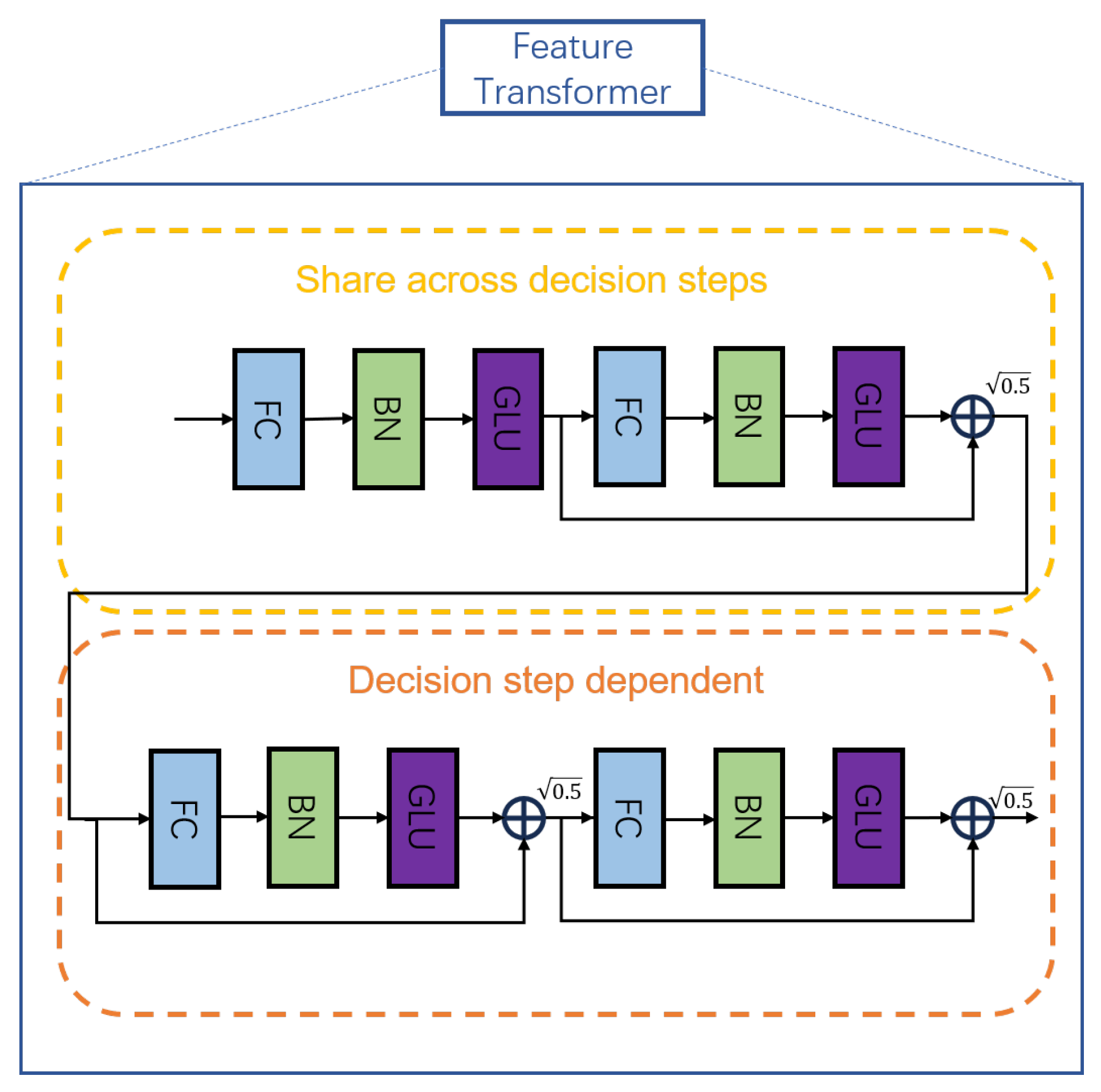
In the Encoder section of the TabNet model (Figure 3), the primary function is to process the input features through a series of decision steps, selectively concentrating on the most relevant attributes for the prediction task. Each decision step consists of two main components: the feature transformer and the attentive transformer. To enhance the feature representation within the TabNet structure, the feature transformer employs an array of FC layers, BN, and Gated Linear Units (PV). These layers combine to map input features into a more useful encoded space. Incorporating normalization, specifically by a factor of $\sqrt{0.5}$, is crucial in this context as it aids in stabilizing the learning process by maintaining consistent variance across the network. This careful calibration ensures that the transformations applied to the features do not induce significant variance shifts, which is vital for the model’s learning stability and overall performance. The attentive transformer then employs a learnable mask, leveraging the $sparsemax$ function to ensure sparsity in the selection of features. This mask is represented mathematically by

$$M\left[i\right]=Sparsemax\left(Z\left[i\right]·a[i-1]\right)$$

(3)

where $M\left[i\right]$ is the mask for step i, $Z\left[i\right]$ is the transformed feature representation, and $a[i-1]$ is the attention from the previous step.

This encoder design enables TabNet to focus on a subset of features at each step, thereby allowing the model to make decisions based on a dynamic and interpretable feature set. This sequential attention mechanism within the encoder is critical for learning complex dependencies and interactions among the features, thereby enhancing the model’s performance on tabular data prediction tasks.

2.4.2. Decoder for TabNet

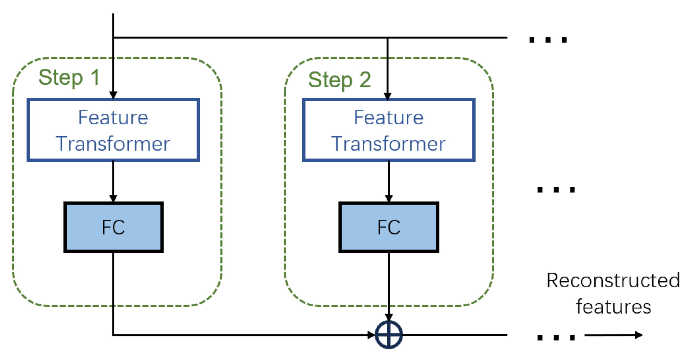
The decoder is crucial in the TabNet model’s self-supervised learning architecture. It is specifically engineered to reconstruct tabular features from the encoded representations. The process is sequential, with each decision step invoking fully connected layers to refine the encoder output Figure 4. The reconstruction of features is informed by a masking array, allowing the model to focus on known features and infer missing ones.

The reconstruction loss function, crucial for the self-supervised learning phase, is carefully formulated to balance the focus between known and unknown features. It is defined in a way that normalizes the error for each feature, weighted by the mask and sums this across all features and instances. This normalization is essential because it accounts for variations in the feature scale. The reconstruction loss is defined as follows:

$$L_{recon}=\sum _{b=1}^B\sum _{j=1}^D{\left|\frac{({\widehat{f}}_{b,j}-f_{b,j})·S_{b,j}}{\sqrt{{\sum }_{b=1}^B{(f_{b,j}-1/B{\sum }_{b=1}^B{f}_{b,j})}^2}}\right|}^2$$

(4)

where the variables are defined within the reconstruction loss function as follows: B is the batch size, D is the dimensional features, ${\widehat{f}}_{b,j}$ is the predicted value for the j-th feature in the b-th sample, $f_{b,j}$ is the true value of that feature, and $S_{b,j}$ is the binary mask indicating feature presence.

The Attention Transformer module within TabNet dynamically allocates focus across features using a mechanism of scaled masks, enabling the model to prioritize information crucial for the current decision step. The $sparsemax$ function aids in this selective attention by producing a mask that acts as a soft selection operator [20], identifying salient features for further processing. In conjunction, the Feature Transformer takes the selected features and applies non-linear transformations through its network layers (Figure 5).This component enhances data representation, allowing TabNet to capture complex interactions and relationships within the features. Collectively, these modules refine the model’s attention and feature processing, significantly contributing to TabNet’s capability to manage and interpret tabular data effectively.

2.4.3. Interpretability of TabNet

TabNet’s interpretability is bolstered by a sophisticated feature selection process that employs both a mask matrix and an importance matrix. The mask matrix, derived from the $sparsemax$ function, is utilized at each decision step to assign a weight to each feature, signifying its importance. The weights are represented by $M_{b,j}\left[i\right]$, which are then factored by the relevance scores ${\eta }_b\left[i\right]$ to form the aggregate mask $M_{\mathrm{agg}-\mathrm{b},\mathrm{j}}$:

$$M_{\mathrm{agg}-\mathrm{b},\mathrm{j}}=\frac{{\sum }_{i=1}^{N_{\mathrm{steps}}}{\eta }_b\left[i\right]M_{b,j}\left[i\right]}{\sqrt{{\sum }_{j=1}^D{\left({\sum }_{i=1}^{N_{\mathrm{steps}}}{\eta }_b\left[i\right]M_{b,j}\left[i\right]\right)}^2}}$$

(5)

In the TabNet architecture, the importance of each feature across decision steps is quantified by the importance matrix I, which is constructed by aggregating the products of the mask matrices $M_{ij}$ and corresponding learnable weights across all steps. This results in a normalized score $I_j$, which conveys the overall significance of feature j in the model’s decision-making process, thereby providing a clear metric for feature relevance and aiding in model interpretability.

$$I_j=\sum _{i=1}^{N_{\mathrm{steps}}}{M}_{ij}{w}_i$$

(6)

Here, $I_j$ signifies the aggregated importance for feature j, accumulated across all decision steps to reflect the feature’s overall influence, enhancing the model’s transparency.

The interplay between the mask matrix and the importance matrix allows TabNet to provide interpretable insights into which features most influence the predictions, fostering trust in the model’s decision-making process.

Table 2. Hyperparameter descriptions.

Hyperparameter	Description
$n_d$	Dimension of the prediction layer
$n_a$	Dimension of the attention layer
$n_{\mathrm{steps}}$	Number of successive steps in the network
$gamma$	Scaling factor for attention updates
$n_{\mathit{independent}}$	Number of independent GLU layers in each GLU block
$n_{\mathit{shared}}$	Number of shared GLU layers in each GLU block
$momentum$	Momentum factor for batch normalization
$lambd{a}_{\mathit{sparse}}$	Coefficient of the L1 sparsity regularization
$mask\_type$	Type of masking function to use for selecting features
$optimize{r}_{\mathit{fn}}$	Optimization function used for training
$optimize{r}_{\mathit{params}}$	Parameters for the optimizer function
$schedule{r}_{\mathit{fn}}$	Learning rate scheduler function
$schedule{r}_{\mathit{params}}$	Parameters for the scheduler function
$batch\_size$	Size of the training batch
$virtual\_batch\_size$	Size of the batches for the virtual BN

lists the hyperparameter and its descriptions. The learning rate scheduler is set to CosineAnnealingLR to speed up the model’s training. Define the optimizer for the model as Adam, which has automatic adjustment capabilities. Set n_d and n_a to determine the model’s complexity, both with default parameters of 12. Increasing n_steps allows the model to analyze the data more deeply, which is set to 10. In this case, a smaller lambda_sparse serves as a sparse regularization parameter, helping reduce redundancy among features. Choose sparsemax as the mask_type to assist the model in focusing its attention on the most important features.

2.5. Evaluation Metrics

In order to evaluate the model performance, the selected evaluation metrics used were mean absolute error (MAE)and root mean square error (RMSE). In addition, this study introduced a key performance evaluation indicator, percentage error (%Er_FT), determined by calculating the percentage difference between the real remaining useful life (RUL_act) and the predicted remaining useful life (RUL_pre) [21]. This indicator directly reflects the degree of variation between the estimated and actual values. It is an important tool for measuring prediction accuracy.

To comprehensively evaluate the accuracy of the model, different fault thresholds (FT) were used in this study, which were 4%, 4.5%, 5%, and 5.5% of the initial voltage, respectively. These thresholds represent the RUL when device performance drops to varying degrees, providing a comprehensive evaluation of the predictive performance of the model under different health states. By calculating %Er_FT under these different fault thresholds, we can more accurately understand the strengths and weaknesses of the model in predicting device health conditions [21].

$$MAE=\frac{1}{n}\sum _{i=1}^n|{\widehat{Y}}_i-Y_i|$$

(7)

$$RMSE=\sqrt{\frac{1}{n}\sum _{i=1}^n{({\widehat{Y}}_i-Y_i)}^2}$$

(8)

$$\%E{r}_{\mathrm{FT}}=\frac{RU{L}_{\mathrm{act}}-RU{L}_{\mathrm{pre}}}{RU{L}_{\mathrm{act}}}\times 100\%$$

(9)

where $Y_i$ is the actual value, ${\widehat{Y}}_i$ is the predicted value, and n is the number of data points.

The percentage error is a crucial indicator of the model’s prediction accuracy, directly reflecting the variance between the forecasted and observed values. A comprehensive evaluation of the model’s accuracy is performed by applying different fault thresholds, representing the RUL at various degrees of performance drop, thus offering an extensive assessment of the model’s predictive capability under diverse health conditions.

3. Experimental Results and Discussion

The TabNet-based PHM system is implemented in the Python programming language. The computational environment is configured as follows:

• Central Processing Unit (CPU): 12th Gen Intel(R) Core(TM) i7-12700H
• Memory: 64.00 GB
• Operating System (OS): Windows 11
• Graphics Processing Unit (GPU): NVIDIA GeForce RTX 3070 Ti Laptop
• PyTorch: 2.1.0
• CUDA: 12.1

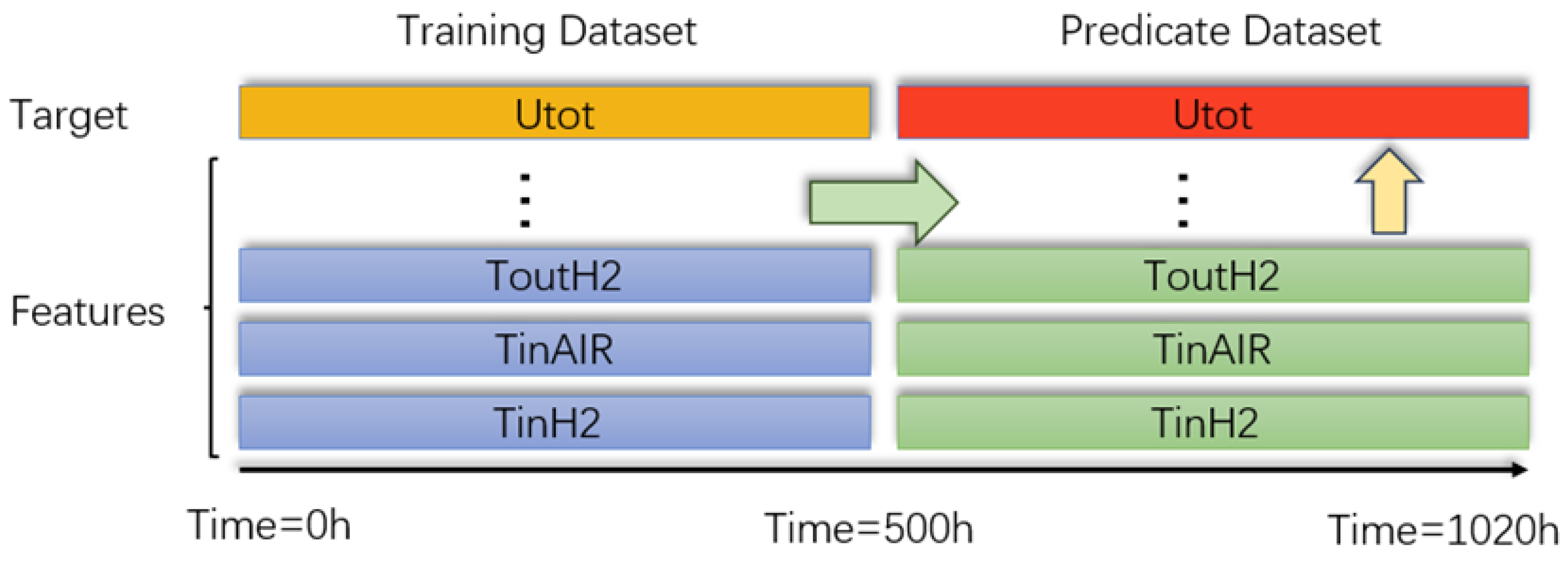
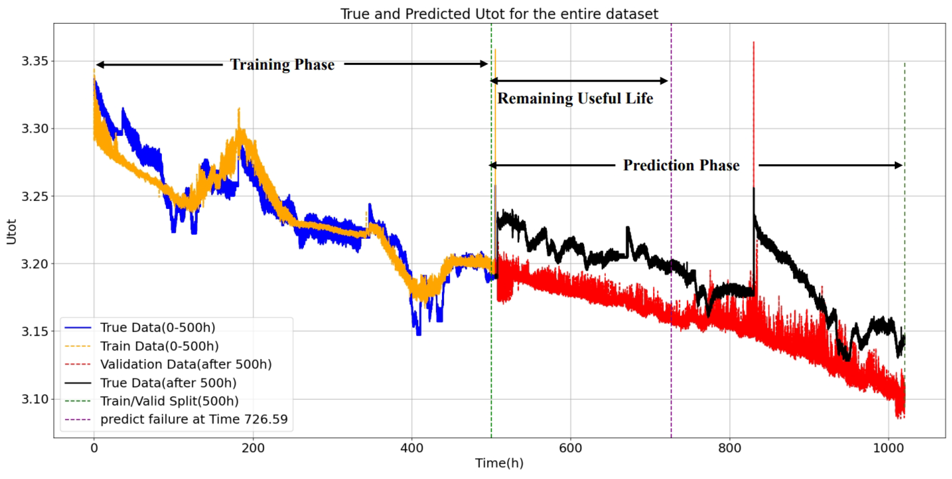
As the data challenge suggested, the first 500 h of data were used to train the model; the rest were for testing. The preprocessed data between 0 and 500 h were fed into the TabNet model, and the HI voltage was the target output. The training and prediction dataset partitioning is shown in Figure 6.

A total of 80% of the first 500 h of the dataset was set for training, and the remaining 20% of it was used to do the validation. A well-trained model was achieved after tuning the hyper-parameters according to this process. To validate the model, an independent dataset was called to help where this dataset was 500–1020 h.

3.1. The Result of Feature Selection

3.1.1. Local Importance

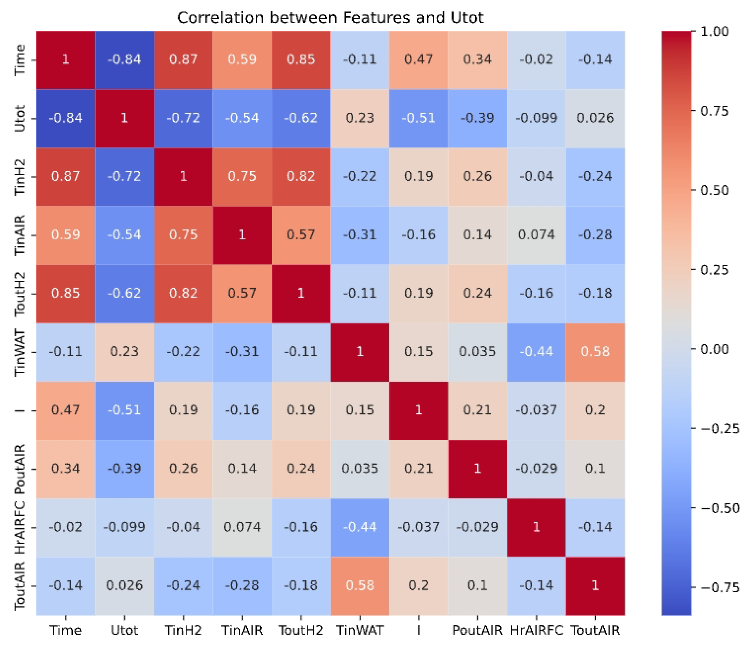
As shown in Figure 7, the degradation of the RUL is determined by a variety of factors, so how to better select the features will be an important factor affecting the performance of the model. A heatmap between the features and the target variable “Utot” was generated to analyze the correlation of the features with respect to the target.

3.1.2. Feature Importance Masks

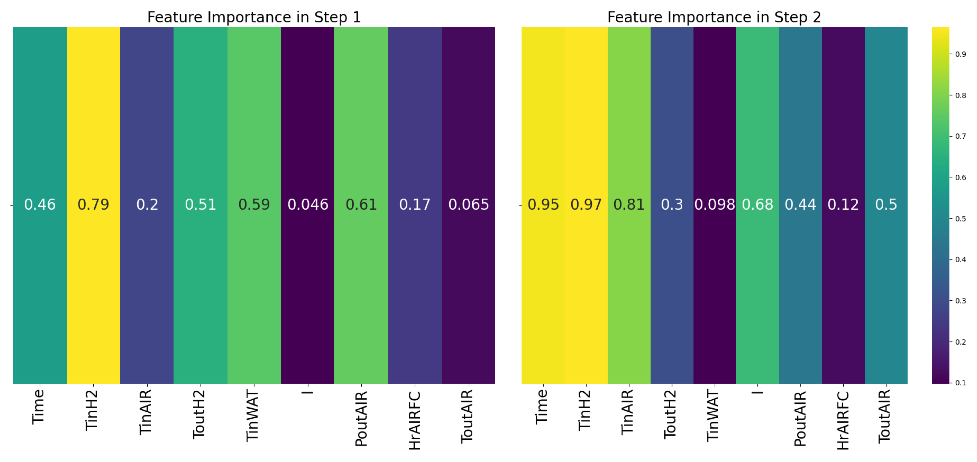
Figure 8 shows what features were selected between the first and second decision steps. The colur from bright yellow to dark purple was assigned to indicate the feature importance to the element in its decision step. Figure 8 also shows that each decision step will assign a different weight to each feature.

3.1.3. Global Importance

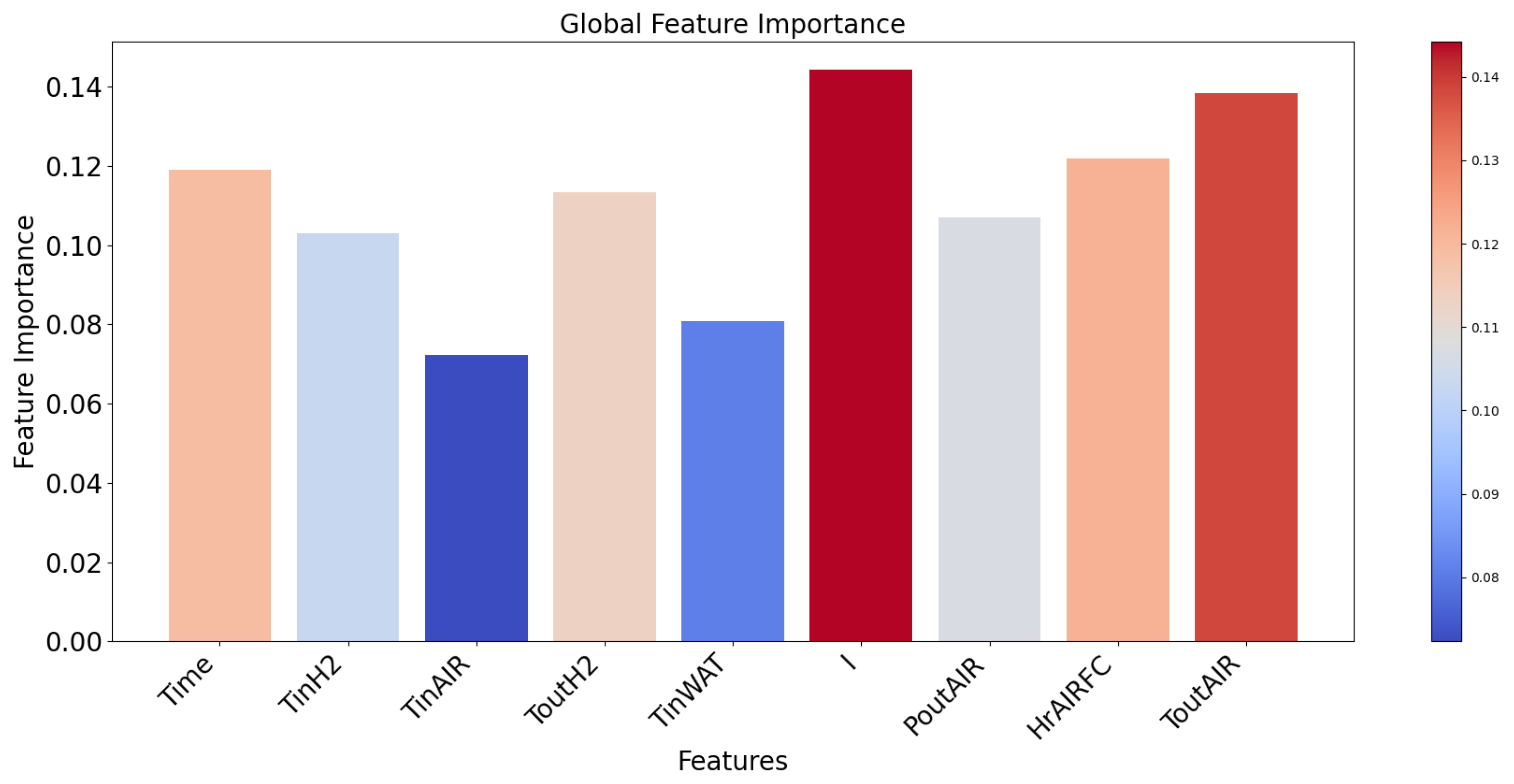
Figure 9 shows the global importance of each feature. TabNet considers the current (I), the outlet air temperature (ToutAIR), the hygrometry of inlet air (HrAIRFC), and the aging time (Time) to be relatively important. These four features account for 51% of the total feature importance.

3.2. Results

The training phase employs data from the initial 0−500 h to train the TabNet model, focusing on stack voltage as the output layer. Subsequently, data spanning 500 to 1020 h were used for the test’s validation, where the model, pre−trained on the earlier dataset, outputs predicted stack voltages. The architecture of the TabNet model is meticulously configured with specific parameters: a decision prediction layer width of 10, an attentional embedding width for the mask also set at 10, and a total of 8 steps within the model architecture. Additionally, it incorporates a feature usage coefficient of 1.3 in the masks and a sparsity loss coefficient set at 1 ×${10}^{-2}$. The model employs the MAE as its loss function, utilizes the Adam optimizer for training, and iterates over 50 epochs with a batch size of 1024. The prediction results, encapsulating the performance of the model across the designated time frames, are depicted in Figure 10.

Advancing into the prediction phase, the model demonstrates commendable proficiency in forecasting voltage degradation. The unity of the predicted and actual $U_{\mathrm{tot}}$ values during this phase reflects the robustness of the model. However, the TabNet system predicts that the PEMFC will prematurely reach the critical failure threshold of 3.158 V at around 729.59 h, whereas actual failure is observed at 922 h. This conservative prediction underscores an exemplary approach to the model but also indicates the potential for refinement to align predictions more closely with actual failure events.

The performance of the model, quantified by an RMSE of 0.0765 and an MAE of 0.0601, corroborates its precision and reliability in predicting the RUL of PEMFCs. These results testify to the capacity of the model to capture degradation patterns despite challenges in predicting the exact timing of failure.

Delving into the specifics of the TabNet architecture, it is apparent that the configuration for feature selection is instrumental in the predictive success of the model. This is particularly relevant for features such as temperatures at the fuel inlet and outlet processed within the decision blocks, which directly correlate with the overall performance of the cell and are integral to the accuracy of RUL predictions.

Table 3. Prediction results of the TabNet model on the test set.

Fault Threshold	Actual Value (h)	Predicted Value (h)	%ErFT	RMSE	MAE
4%	220	0	100%	0.0765	0.0601
4.5%	258.5	11	95.8%	-	-
5%	422	226.5	46.3%	-	-
5.5%	435.5	333.5	23.3%	-	-

presents an in-depth look at the predictive accuracy of the model across various fault thresholds. The presented data delineate the consideration of four distinct power reduction thresholds—4%, 4.5%, 5%, and 5.5%. The objective was to ascertain these specific decrements in power prior to forecasting the remaining operational duration. For instance, to achieve a 4% power drop, the actual operating time (expressed in hours) is computed as 220, deduced from 720 by subtracting 500 h, by the following formula: Actual value at 4% = 720 − 500. This subtraction is predicated on the dataset’s continuity and aims to facilitate a comparative analysis of power reductions post the 500 h mark.

For the aforementioned failure thresholds (FT), the calculated %Er_FT are as follows: 100% (at 4%), 95.8% (at 4.5%), 46.3% (at 5%), and 23.3% (at 5.5%). Notably, the minimum %Er_FT is observed at the 5.5% FT. Subsequent to the 500 h interval, predictions encompassing the entire dataset were executed. This was accomplished by initially pre-training the model, which subsequently enabled the determination of two critical parameters for assessing the regression model’s performance—RMSE and MAE, which were computed to be 0.0765 and 0.0601, respectively.

The table illustrates that while the model maintained a reasonable margin of error across all thresholds, accuracy improved at higher fault levels, with the lowest percentage error recorded at the 5.5% threshold.

The TabNet-based PHM system, through adept feature selection and predictive modeling, holds significant promise for monitoring PEMFCs. While currently erring on the side of caution by predicting earlier failure points, ongoing enhancements to the calibration of the model could further sharpen its timing accuracy. This continued development aims to bolster the practicality of the system for real-world applications, ensuring reliable and timely maintenance decisions.

4. Conclusions and Future Work

The research conducted in this study demonstrates the substantial potential of integrating TabNet into PHM systems for PEMFCs. Applying SRSC and Gaussian augmentation in data preprocessing has proven effective in enhancing the model’s performance and accuracy. TabNet’s ability to discern critical features and patterns in sequential tabular data plays a pivotal role in the precise prediction of RUL, contributing to more reliable and explainable PHM systems. The results indicate that while the model is currently conservative in its predictions, ongoing refinements could improve its precision, particularly in aligning predicted failure events with actual occurrences. This advancement in PHM systems using TabNet not only supports the longevity and reliability of PEMFCs but also underscores the growing importance of machine learning techniques in the renewable energy sector. Future work will further optimize the model to reduce prediction errors and adapt the system to broader applications in renewable energy technologies.