Article

Enhancing Anomaly Detection for Cultural Heritage via Long Short-Term Memory with Attention Mechanism

1
College of Computer Science and Technology, Zhejiang University, Hangzhou 310027, China
2
China Mobile Group Zhejiang Company Limited, Hangzhou 311100, China
*
Authors to whom correspondence should be addressed.
Electronics 2024, 13(7), 1254; https://doi.org/10.3390/electronics13071254
Submission received: 21 January 2024 / Revised: 7 March 2024 / Accepted: 16 March 2024 / Published: 28 March 2024

Abstract

:
Cultural heritages are invaluable and non-renewable resources. Existing warning mechanisms usually rely on degradation analysis to assess environmental risk factors. However, they have limitations such as complex research, poor generalization, and inadequate warnings. To address these issues, we propose a hybrid model that combines the long short-term memory network (LSTM) and attention mechanisms with environmental factors to detect anomalies in cultural heritage. The attention mechanism extracts temporal dependencies, while LSTM captures global long-term patterns, enhancing the reconstruction capability. Additionally, we introduce the seasonal, trend, shapelet, and mixed anomalies to enrich the positive and negative samples and propose a novel threshold extraction method to reduce the reliance on prior knowledge. Extensive experiments demonstrate that LSTM-Attention outperforms previous methods, with a root mean square error (RMSE) of 34.328, mean absolute error (MAE) of 27.060, and the largest area under the receiver operating characteristic curve (AUC) value, highlighting the superiority and effectiveness of our method. The ablation study proves the contribution of the attention mechanism, and the reconstruction step can be flexibly adjusted according to practical needs. Finally, the algorithm has been successfully implemented in engineering and employed in practice, providing valuable guidelines for the preservation of ancient buildings worldwide.

1. Introduction

Cultural heritage represents a profound embodiment of human civilization, holding significant artistic and scientific value [1]. Yet, ancient buildings face numerous influences, including the passage of time, environmental fluctuations, and human activities. Consequently, these structures often contend with underlying challenges, such as structural fissures, erosion, and morphological distortions. These issues not only endanger the structural integrity of ancient buildings but also cast a shadow over the historic preservation and cultural legacy. Current preventive strategies primarily revolve around a meticulous analysis of the root causes of degradation. This involves the construction of finite element stress analysis models grounded in the building’s framework and executing simulation experiments to validate and refine these models [2,3]. Subsequently, warning thresholds were derived from the model analysis results. Despite these assiduous endeavors, establishing an efficacious early warning system for heritage monitoring remains a formidable challenge, given the limited comprehension of the intricacies underpinning degradation mechanisms. Furthermore, the copious stream of monitoring data available is inadequate in furnishing timely guidance and support for contemporary heritage conservation undertakings. Thus, a pressing and compelling need exists in heritage conservation that transcends the constraints inherent in traditional methodologies.
Early anomaly detection is crucial for safeguarding cultural heritages against the insidious threat of deterioration [4,5,6]. Traditionally, previous studies have been conducted in cultural heritage conservation utilizing the degradation causation analysis [7,8,9]. This method involves meticulously examining the deterioration mechanisms inherent to heritage materials. Through extensive simulation experiments, researchers delve into the degradation process of heritage materials under specific conditions, aiming to identify factors that can mitigate deterioration challenges while establishing corresponding threshold values. For instance, Liu et al. [10] elucidated the microbial degradation process concerning stone monuments and structures, providing a detailed account of biofilms’ progression and succession on cultural heritage surfaces. Similarly, Qu et al. [1] probed the effect of freeze–thaw cycles and wind erosion on earthen sites in northwestern China, systematically exploring the relationship between soil wind erosion strength, freeze–thaw cycle frequency, water content, and moisture levels by carefully designed simulated trials. Their findings yielded valuable insights into reinforcement materials capable of regulating freeze-thaw cycles and moisture levels, enhancing the resistance of soil sites against wind erosion. Riccardo Fanti et al. [11] harnessed three-dimensional models attained via terrestrial laser scanning. They executed structural force analyses grounded in these models, predicted outcomes through simulated experiments, leveraged these predictions as benchmarks, and employed ground-penetrating radar to detect anomalies deviating from the projected outcomes. However, despite the invaluable insights gained from early warnings based on degradation causation analysis, it is imperative to acknowledge the inherent limitations of this approach, including its complexity and limited generalizability. Typically conducted in controlled laboratory settings, this method presents a significant disconnect between laboratory conditions and real-world field settings, resulting in substantial disparities that impact the reliability of inferences drawn from experimental results. Additionally, it necessitates extensive simulations under precisely defined conditions to establish anomaly thresholds, which places resource-intensive demands and results in poor generalization performance. Consequently, setting early warning thresholds based on deterioration mechanisms proves challenging, impeding the effective utilization of monitoring data to detect anomalies in ancient buildings early. Furthermore, the feasibility of implementing this approach on a per-artifact basis is curtailed due to the diverse and distinctive attributes encompassing material composition, temporal aging, and environmental context. This, in turn, limits its broader applicability and generalizability.
The evolution of monitoring technologies has yielded a substantial influx of data, and various industries capitalize on data analysis to achieve effective outcomes. This advancement trajectory offers a salient proposition for the surveillance and preservation of historical edifices. This momentum has, in turn, paved the way for the advent of early warning paradigms underpinned by statistical analysis, correlation evaluation, and machine learning techniques. These approaches have found application across various contexts, as evidenced by numerous studies. For instance, Milan Holický et al. [12] conducted a statistical analysis of the Vltava River’s annual maximum flow monitoring data in Prague. They employed normal distributions and Pearson fitting, utilizing moment and maximum likelihood estimations to derive probability distributions. Dennis M. Staley et al. [13] leveraged rainfall, hydrologic response, and geospatial data to devise a predictive model for debris flow hazard thresholds, hinging on rainfall intensity, duration, and probability. Other investigations employed machine learning strategies, including differential autoregressive moving average algorithms, Long Short-Term Memory (LSTM) networks, and backpropagation neural networks (BPNN). Liang et al. [14] implemented differential autoregressive moving average models to anticipate oil pressures and establish pressures within the confines of industry-specific thresholds for an early warning framework. Giovanni Gigli et al. [15] formulated a landslide early warning model by analyzing monitoring data preceding a landslide event. Xie et al. [16] utilized LSTM networks to predict the cyclical component of landslides, considering geological conditions, rainfall intensity, and human activities. Their monitoring outcomes exhibited robust consistency, addressing the multifaceted influences on landslide displacement and providing guidance for early warnings. Fan et al. [17] employed a BPNN to predict failures in smart grid equipment. The network assimilated monitoring data from diverse influencing factors of the equipment in question to predict the probability of equipment failure. Moreover, other inquiries embraced some other anomaly detection methods. Zhu et al. [18] applied K-means clustering to scrutinize rockburst monitoring data and offered tiered warnings based on clustering results. Chen et al. [19] introduced a novel multivariate time series anomaly detection framework that introduced graph convolution for detecting anomalous information flow between IoT device nodes. In the industrial IoT context, Gauri Shah et al. [20] employed diverse machine-learning techniques to model data anomalies. Collectively, these above studies manifest continuous endeavors to enhance early warning techniques, contributing substantial insights to heritage preservation.
Nevertheless, previous studies have focused on identifying and categorizing damage to ancient buildings. They do not adequately address the issue of incorporating anomaly data into the dataset, which is essential for practical building preservation. Anomalies detection of ancient buildings is a multifaceted endeavor that encompasses various scales and degrees of characterization. Anomalies in such structures can manifest in specific areas, ranging from structurally fragile parts to historically significant zones. The aforementioned methods may not effectively cover the intricate interrelationships inherent in these features. In contrast, the incorporation of attention mechanisms offers a promising approach to address these complexities. Attention mechanisms allow models to discern significant attributes across diverse scenarios, allowing them to capture anomalous subtleties and features skillfully. The ability of the mechanisms to focus on critical regions enables the model to understand the nuances associated with specific anomalies and to adapt to different anomaly patterns. Furthermore, temperature and humidity may impact the material properties and structural behavior of buildings over time. For instance, temperature variations may cause the expansion or contraction of building materials, while humidity changes can lead to swelling or warping. The relationship between the building structure and the environment is subject to change due to anomalies. The incorporation of temperature and humidity as external influence features into the model can enhance the accuracy of anomaly detection for ancient buildings. As a result, they improve the accuracy, adaptability, and generalizability of the model’s anomaly detection process.
Thus, in this study, our objective is to enhance anomaly detection accuracy. First, we introduce an anomaly data augmentation strategy, which includes seasonal, trend, shapelet, and mixed anomalies to enrich our dataset with positive and negative samples. Subsequently, we integrate the attention mechanism with LSTM to build an LSTM-Attention model. In addition, we propose a novel threshold extraction method based on extreme value theory and recurrence interval calculation. The experimental results demonstrate that our algorithm can effectively detect anomalies in ancient buildings, making it a practical and effective solution for preventing potential damages. To be specific, the contributions are as follows:
(1)
We propose a novel algorithm for early warning of anomalies in ancient buildings by combining environmental factors with the building structure to improve prediction accuracy.
(2)
We introduce the seasonal, trend, shapelet, and mixed anomalies to increase the positive and negative samples of the datasets.
(3)
We incorporate the attention mechanism into the domain of ancient buildings and combine it with LSTM architecture to more effectively extract the inherent characteristics of monitoring data, particularly temporal dependencies, enhancing model prediction accuracy. To our knowledge, this investigation is one of the initial endeavors that delve into the augmentation of anomaly data and the application of attention mechanisms in the context of anomaly warning tasks for ancient buildings.
(4)
We propose a novel threshold extraction method based on extreme value theory and recurrence interval calculation, which reduces reliance on prior knowledge and allows for the extraction of different warning threshold intervals automatically.
(5)
We implement and deploy the anomaly warning program, making it applicable and providing guidelines for conserving cultural heritages in other locations.

2. Materials and Methods

2.1. Experimental Data Acquisition

2.1.1. Experimental Data

The dataset utilized in this study is from Baoguo Temple, located in Ningbo, Zhejiang Province, and involves horizontal displacements of tenons in an ancient building structure. These data come from an Internet of Things (IoT) monitoring system specifically designed to monitor anomalies in ancient buildings. Figure 1 intuitively shows the exact location of the tenon displacement sensor, which is used to track the displacement of the tenons in wooden structures. Adjacent to the tenon displacement sensor, humidity and temperature sensors were strategically deployed to complement the measurement framework. Furthermore, other installation locations in the figure were carefully selected to collect monitoring data from artifacts in different building areas.
To evaluate the effectiveness of our anomaly warning algorithm, a specific period from 5 August 2019, to 12 June 2020, was chosen for analysis using displacement data, with all sampling intervals of 2 h and 4217 cumulative data. For validation, part of the original data corresponding to 10 October 2019, was selected and is presented in Table 1.

2.1.2. Anomalous Data Synthesis

The ancient architectural artifacts typically exhibit a high degree of stability in their day-to-day conditions, it is true that the anomalous data is pretty limited. However, it is precisely because of this stability that anomalies, when they do occur, may signify critical deviations from the norm and potentially indicate underlying issues that require immediate attention. Thus, additional anomalies were introduced to augment the dataset and evaluate the model’s robustness and generalization ability becomes essential for training anomaly detection models effectively, including seasonal, trend, shapelet, and mixed anomalies [21], which can better enhance its overall performance and ensure the robustness of the anomaly detection system in safeguarding cultural heritage assets. The relevant parameters for the synthesis process are presented in Table 2. In the case of mixed anomalies, the parameters α and β were reduced by half of their original values to avoid excessive prominence when superimposed. Part of the resulting dataset is signified in Figure 2.
(1)
Add seasonal anomalies. As shown in Equations (1) and (2), the seasonal anomaly is introduced by adding the original series to the series of other periods.
S ¯ seasonal = S + α · ρ seasonal ( ω ^ I ) · g ( I ) + ε
g ( x ) = x a x a 1 x > a
where S R l × d 1 is the original building sequence. I = { 1 , 2 , , l } R l × 1 is the incremental sequence. l is the sequence length, and  ω ^ is the anomaly period. ρ seasonal is the sine function; g is the transition function to model the process of sequence correlation change caused by adding anomalies, and a is half of l. α is used to adjust the effect of anomalies on the original sequence, and  ε is random noise.
(2)
Add trend anomalies. The trend anomaly is applied by summing the original series with a monotonically increasing or decreasing series, as shown in Equation (3).
S ¯ trend = S + β · I · g ( I ) + ε
where β is used to moderate the effect of the outliers.
(3)
Add shapelet anomalies. The shapelet anomaly is introduced by adding the original sequence to another sequence with the same period, as shown in Equation (4).
S ¯ shapelet = S + γ · ρ shapelet ( ω ^ I ) · g ( I ) + ε
where ρ shapelet is a sine function, γ is the period of the original sequence. is used to regulate the effect of shapelet anomaly on the original series.
(4)
Add mixed anomalies. The mixture of seasonal, trend, and shapelet anomalies is introduced simultaneously, as shown in Equation (5).
S ¯ mix = S + S ¯ seasonal + S ¯ trend + S ¯ shapelet
To balance the number of positive and negative samples in the test set after introducing synthesized anomalies, we adopt the alternating introduction method for each anomaly class. Assuming that the original test set contains n normal samples, numbered 1, 2, ⋯⋯, n, then for sample number i, the following rules are used to introduce anomalies:
(1)
For the sample with code i mod 4==0, a shapelet anomaly is introduced.
(2)
For the sample with code i mod 4==1, a seasonal anomaly is introduced.
(3)
For samples with code i mod 4==2, a trend anomaly is introduced.
(4)
For the sample with code i mod 4==3, a mixed anomaly is introduced.
This method ensures an equal number of positive and negative samples in the synthesized anomaly dataset.

2.2. The Attention Mechanism

Inspired by the human brain’s attention mechanism, the attention mechanism selectively weighs critical information from a large amount of data to enhance neural network efficiency. This mechanism has found extensive applications in various domains, including sentiment analysis [22,23], image segmentation [24,25], intelligent recommendation [26,27] and time series forecasting [28,29,30]. The self-attention mechanism, a prominent component of the transformer model developed by the Google team [31], is a variant of the attention mechanism. The attention mechanism reduces the dependence on external information and excels at capturing internal data relationships. For anomaly detection tasks, it possesses the capability to autonomously learn and assign weights to features based on their intrinsic relevance within the data, focusing on those essential features to improve the accuracy of anomaly detection. Moreover, it facilitates the capture of contextual information present in the data while effectively mitigating the interference caused by noise and anomalous data points, boosting model performance and robustness significantly. As displayed in Figure 3, input data is typically described in terms of Query, Key, and Value, and the computation process can be outlined as follows.
  • Data input. A linear transformation can map the input sequence to Query, Key, and Value.
  • Calculate the correlation. The correlation between the Key and Query is calculated and normalized, and the attention distribution of critical values is obtained using the softmax function.
  • Weighted summation. According to the attention distribution calculated in step 2, the corresponding Value is weighted and summed to obtain the output.
The calculation of the self-attention is similar to the traditional attention mechanism; the difference is that in step 1, the Query, Key, and Value of the self-attention come from the same input sequence, which is a linear transformation of its input. Generally speaking, self-attention uses the scaled dot product for correlation calculation, and the self-attention equation is shown as follows.
A t t e n t i o n ( Q , K , V ) = S o f t m a x ( Q K T d k )
where d k represents the dimension of the input data.

2.3. Long Short-Term Memory Network (LSTM)

LSTM is a variant of the traditional recurrent neural network (RNN) that can effectively learn long-term dependencies and achieve better results in time series forecasting [32]. Nowadays, LSTM has been applied in many fields, such as language modeling [33,34], time series forecasting [35,36], and automatic speech recognition [37,38]. The primary structure of the LSTM cell is shown in Figure 4.
LSTM regulates the information flow by introducing gate mechanisms as internal gating units, including input gates i t , forget gates f t , output gates o t , and state vector C t , which can achieve the long-term memory and solve the gradient disappearance and gradient explosion problems. The forget gate f t determines the information to be remembered and discarded in C t 1 by using the previous cell output vector h t 1 and the current input vector x t . Additionally, the input gate i t controls what information is updated to the new cell state C t . Finally, combine C t with o t to determine the final output [39]. The LSTM is formulated as
f t = σ ( W f x x t + W f h h t 1 + b f )
i t = σ ( W i t x t + W i h h t 1 + b i )
μ t = t a n h ( W μ x x t + W μ h h t 1 + b μ )
C t = f t C t 1 + i t μ t
o t = σ ( W o x x t + W o h h t 1 + b o )
h t = o t t a n h ( C t )
In the formulas, x t is the input vector, h t is the memory cell output, σ , and tanh are activation functions. W and b represent the weight and bias of the neural network, respectively.

2.4. The LSTM-Attention Framework

The attention mechanism was proposed to allow the model to focus on specific input parts. It was used to enhance LSTM performance in many applications by assigning attention scores for LSTM hidden states to determine the importance of each state in the final prediction [40,41]. Attention mechanisms can be more effective with long sequences, and they can improve the interpretability of the model. The network structure of the LSTM-Attention model proposed in this paper is schematically shown in Figure 5. The figure contains four parts: (1) cutting displacement and environment data, (2) extracting global temporal features in the window, (3) extracting time series dependencies, and (4) reconstructing the recent displacement data.
  • Cut the displacement and environmental data. In this paper, the displacement and the environmental data are cut to the same size as the sliding window. As shown in the blue dashed box part of the figure, the different colored origin points represent different time series. The sliding window size is W × D, W is the period of the sliding window, and D is the time series dimension. The sliding window moves along the time axis, and the data set in the red box part is obtained after cutting. The small black box is the recent displacement data used as the training set label.
  • Extract global time features. LSTM has an excellent performance in long sequence tasks, which is well-suited for cultural heritage where data often exhibits temporal dependencies. This paper uses LSTM to extract the time series features in the window, capture and learn from the temporal patterns, and output the hidden state values to prepare for the subsequent calculation of the weights of each hidden in the self-attention layer, enabling it to discern anomalous behavior over time.
  • Extract dependencies of time series. The attention mechanism enhances the LSTM model’s ability to focus on relevant information within the input sequences. This is particularly beneficial for anomaly detection tasks where subtle deviations from normal behavior need to be identified. Reasonable allocation of attention weights can effectively improve the reconstruction ability of the model. The self-attention allocates more weight to the key parts that affect the output more, which can improve the model’s interpretability. The sequence of hidden state values in LSTM contains the environment sequence and the ancient building sequence. Actually, calculating the weight matrix is extracting the dependencies between the time sequences, thereby improving the accuracy of anomaly detection.
  • Reconstruct the recent displacement data. Extract the association between features and map them to the output, which will reconstruct the recent displacement data.
We combine LSTM with the attention mechanism to effectively leverage the temporal dynamics of the data while attending to salient features, enhancing its capability for detecting anomalies in cultural heritage. The LSTM-Attention model leverages the next period’s environmental data to constrain the reconstruction of the next period’s displacement data. It offers flexibility in adjusting reconstruction intervals within a single iteration to align with practical requirements. However, it is crucial to emphasize that despite the LSTM-Attention possessing the capability to handle extended reconstructions by manipulating input-output dimensions, it often encounters prolonged convergence time and reduced precision during the reconstruction process. To mitigate these challenges, this paper introduces a multi-step reconstruction approach. Initially, it involves reconstructing a period of displacement data. Subsequently, this reconstructed displacement data is employed as historical input, combined with subsequent environmental data as inputs. The model then reconstructs the displacement for the next period. The effectiveness of this approach critically hinges on the regulation of the time window and the reconstruction steps, which ensures the model’s competence in executing protracted reconstructions effectively.

2.5. Model Anomaly Threshold Extraction

An anomaly threshold extraction algorithm based on extreme value theory (EVT) and recurrence interval calculation (RIC) is proposed. The pseudocode is shown in Algorithm 1. EVT is commonly used to predict the probability of extreme events, and one important tool is the generalized extreme value distribution. It extensively involves hydrology [42,43], meteorology [44], finance [45,46], and is calculated through Equation (13).
G γ ( x ) = exp 1 + γ x μ σ 1 γ , γ 0 exp exp x μ σ , γ = 0 , γ R , 1 + γ x μ σ > 0
where μ is the position, σ is the scale, γ is the shape.
RIC refers to the average interval between extreme events, which occurs once in N years, playing a vital role in determining the extreme event probability α for threshold extraction calculated by Equations (14). RIC measures the danger level of extreme events. In general, larger N corresponds to smaller α , resulting in higher danger levels. Thus, adjusting N allows for the anomaly threshold extraction at different danger levels.
α = 1 365 · N
Algorithm 1: Threshold extraction.
Input:  Err normal : Prediction error set N: Recurrence period G: Extreme value distribution function
1. ρ 1 = KSTest ( Err normal , Gumbel ) // Test Gumbel extreme value distribution
2. ρ 2 = KSTest ( E normal , Weibull ) // Test Weibull extreme value distribution
3. ρ 3 = KSTest ( E r r normal , Frechet ) // Test Frechet extreme value distribution
4. G = select G ( ρ 1 , ρ 2 , ρ 3 ) // Select the distribution function based on the p
5. ( γ , μ , σ ) = fit ( G , E normal ) // Fitting the distribution
6. c d f ( x ) = x G ( x , γ , μ , σ ) , d x // Calculate the cumulative probability density distribution
7. α = 1 365 · N // Calculate the probability of the extreme events
8. τ = c d f 1 ( 1 α ) // Calculate the threshold value based on the inverse function of c d f ( )
9. return  τ
Output: τ

2.6. Model Performance Criteria

To further compare the model’s performance in this paper with other models, two criteria are selected: root mean square error (RMSE) and mean absolute error (MAE).
The expression for RMSE is shown below:
RMSE ( X , h ) = 1 m i = 1 m h x ( i ) y ( i ) 2
The expression for MAE is shown below:
MAE ( X , h ) = 1 m i = 1 m h x ( i ) y ( i )
where m is the total number of test sets, h ( x ) is the reconstructed value, and y is the actual value. A lower the RMSE and MAE indicate a more accurate model.
The R O C curve is used to verify the ability of the model to detect anomalies. T P R is the ratio of positive cases, and F P R is the ratio of negative cases. The calculations are in Equations (17) and (18), where the meanings of T P , F P , F N , and T N are shown in Table 3.
T P R = T P T P + F N
F P R = F P F P + T N
The lower half area of the ROC is the AUC value. The larger the AUC value, the better the anomaly detection effect.

3. Results

3.1. Risk Source Selection

This paper uses scatter plots to select the critical factors for risk sources. From Figure 6, it can be seen that there is a specific linear relationship between humidity and tenon displacement. In contrast, the relationship between temperature and tenon displacement is not apparent.
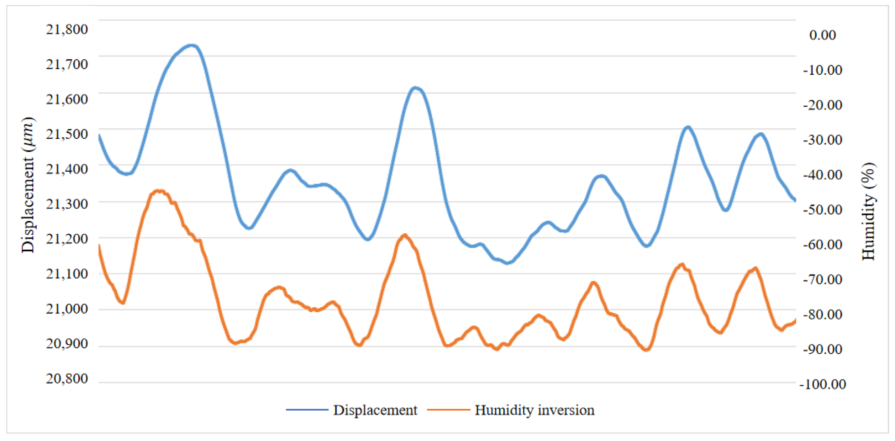
Moreover, we employed the Spearman correlation coefficient to discern the environmental data points whose correlation values with tenon displacement fell from −0.5 to 0.5. Notably, the correlation coefficient between humidity and tenon displacement was computed to be −0.75, while the correlation coefficient between temperature and tenon displacement stood at 0.23. Humidity exhibited a more pronounced correlation with tenon displacement. To visualize the correlation between the tenon displacement and the humidity, the monitoring data was preprocessed in the experiments, including filtering to eliminate some noise effects and inverse operation on the humidity. As depicted in Figure 7, the robustness of the correlation between humidity and displacement is evident, accentuated by a discernible hysteresis effect in the influence of humidity on displacement. Therefore, we selected humidity as a significant influencing factor, with ensuing discussions aimed at elucidating the hysteresis phenomenon exhibited by humidity’s impact on displacement.

3.2. Hysteresis Analysis

Hysteresis manifests in the relationship between humidity and tenon displacement, thereby necessitating the determination of an optimal lag time denoted as ’d’ to capture this effect.
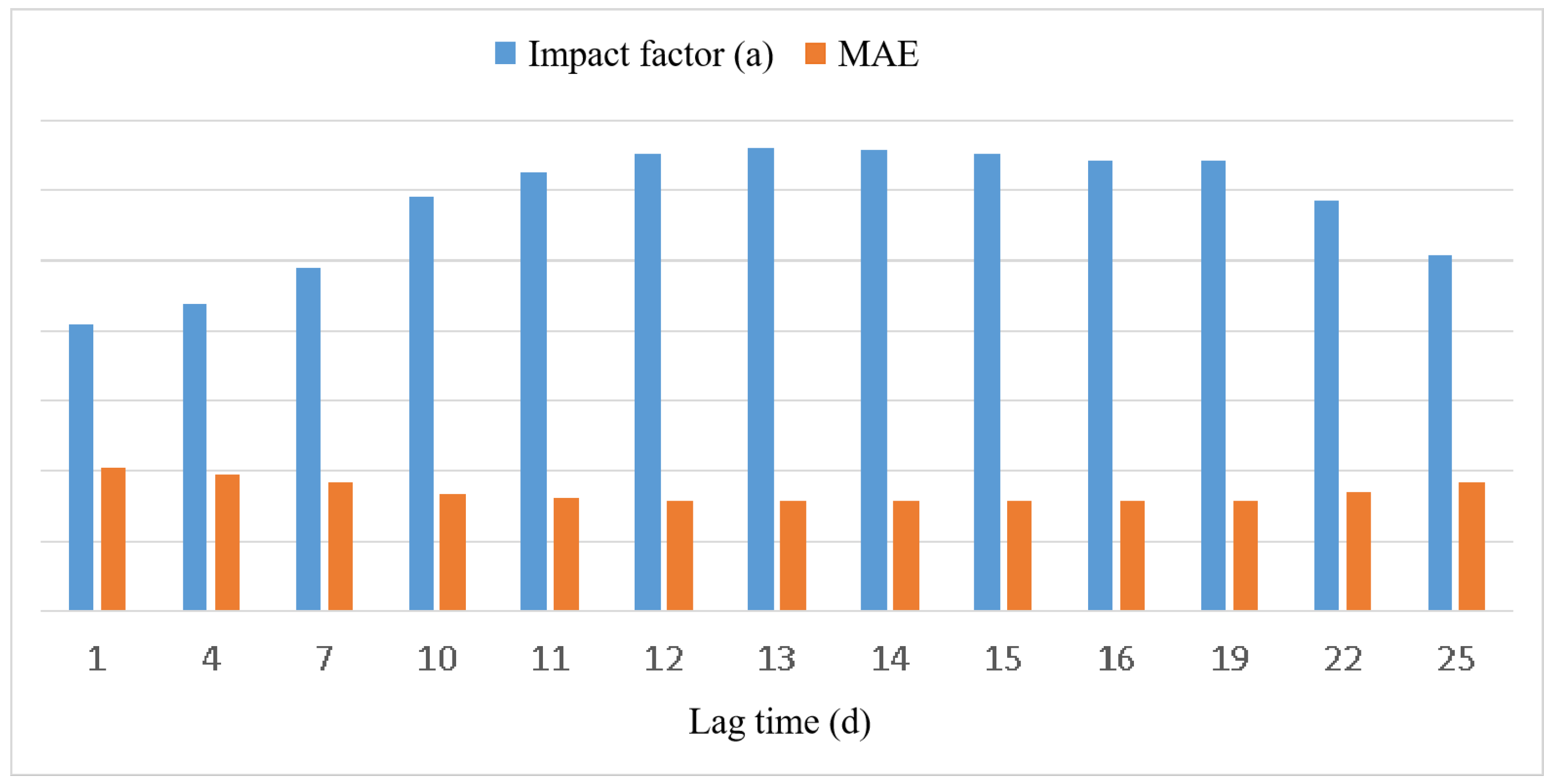
The outcomes of the lag analysis are depicted in Figure 8. In this representation, ’d’ denotes the lag time, while ’a’ signifies the magnitude of humidity’s influence on tenon displacement. Within the hysteresis interval [1,25], with the progression of lag time ’d’, the factor ’a’ initially ascends before subsequently descending. Simultaneously, the MAE follows a trajectory of decline followed by ascent. Remarkably, when the lag time ’d’ equals 13, the factor ’a’ attains its zenith while the MAE reaches its nadir. Given the two-hour sampling interval, the lag time range associated with humidity’s impact on tenon displacement spans approximately 26 h (about one day). This interval is a pivotal reference in determining the temporal window length for the LSTM-Attention model.

3.3. Parameter Sensitivity Analysis

3.3.1. Parameter Sensitivity of Time Window and Reconstruction Step

The LSTM-Attention model’s training process involves a batch size of 64 and is trained over 100 epochs using the Adam optimizer. The model also requires two key parameters: the time window and the reconstruction step. These parameters are selected through a comparative analysis of multiple experiments. In this study, the time window length was investigated within the range of [6,20], and the reconstruction step was explored within the range of [1,20]. The subsequent figures illustrate the correlation between the time window, the reconstruction step, and the model’s evaluation metrics.
As inferred from Figure 9, the time window lengths exert a palpable influence on the reconstruction accuracy. Both reconstruction evaluation indices exhibit a trend of initial decrease, followed by an increase as the time window length escalates. Notably, the reconstruction errors reach their nadir when the time window length is 14, thereby leading us to fix the time window length at 14. On the other hand, the depiction in Figure 10 reveals a consistent trend across the two reconstruction evaluation indices, demonstrating a linearly increasing pattern. This implies that setting a longer reconstruction step for a given iteration results in an enlarged reconstruction error for the LSTM-Attention model. Consequently, the reconstruction step is optimally positioned to 1.

3.3.2. Parameter Sensitivity of Data Synthesis

Our research aims to develop an anomaly detection algorithm for ancient buildings by combining LSTM modeling and anomaly data synthesis. Due to the limited historical anomaly data of different types of ancient buildings, we synthesized a large number of additional anomaly sequence data by processing various anomaly parameters. To ensure the accuracy of the synthesized data, we collaborated with two well-known organizations and formed a team of experts in the field. After conducting synthesized experiments, we submitted the results to experts for validation. These experts used their understanding of the structural mechanisms and anomaly data of that particular ancient building to validate and confirm the parameter values. Subsequently, we implemented these parameter values in an anomaly detection system with favorable results.
The parameters α , β , and γ measure the effect of seasons, trends, and shapelets on the original sequence. We study the effect of different parameter values α , β , and γ on the model’s performance using time step = 400. During the analysis, we hold the other parameters constant to understand the impact of these parameters better. By analyzing the values of the parameters α , β , and γ , we further investigated the effect of the parameters on the model performance. We analyzed the effect of varying values for (0.05, 0.1, 0.2, 0.3, 0.4), (0.001, 0.005, 0.01, 0.02, 0.03), and (0.05, 0.1, 0.2, 0.3, 0.4) on the model’s performance. The quantitative values of MAE and RMSE corresponding to different parameter values are presented in Table 4, Table 5 and Table 6. The results show that the model performance is higher when the α is set to 0.2. Figure 11a shows the variation of these metrics with varying α values. The model metrics do not change much with different parameters, proving that our model performs strongly with other parameters.
Table 5 provides the quantitative values, while Figure 11b visualizes the variation of the metrics at different values of parameter β . The results show that MAE is the lowest when β is set to 0.005, but the results are also satisfactory when β is set to 0.001, which suggests that the model is still feasible for more minor anomalies. Similarly, the quantitative values are presented in Table 6, and Figure 11c shows the visualization of the metrics for different γ . The results show that MAE is the lowest when γ is set to 0.2, but the results are also satisfactory when γ is set to 0.4, which suggests that the model is still feasible for more prominent anomalies. The analysis shows that the model is robust to parameter variations.

3.4. Validity Analysis

To validate the effectiveness of the proposed LSTM-Attention model, a test set comprising 300 samples was utilized. According to the parameter settings of a time window length of 14 and reconstruction step size of 1, the reconstruction is carried out for 400 steps.
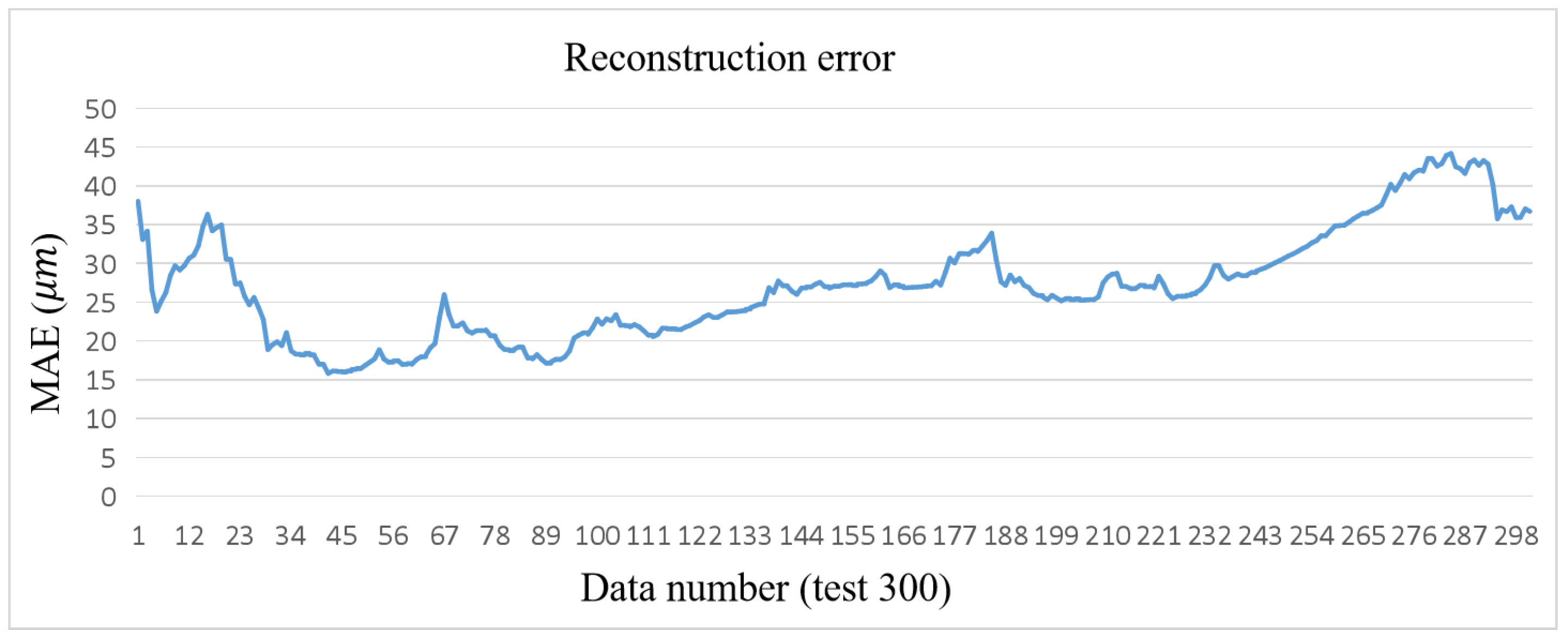
As depicted in Figure 12, the trained LSTM-Attention model successfully maintains the reconstruction error (MAE) within 45 μm for the validation set. This outcome indicates that the model effectively captures the correlation between the structural elements and the environmental conditions, enabling accurate reconstruction of the data about ancient architectural relics based on recent environmental data. Furthermore, the stable range of the reconstruction error allows for the extraction of anomaly warning thresholds, which facilitates the implementation of anomaly detection and warning systems.

3.5. Necessity Analysis of External Factors

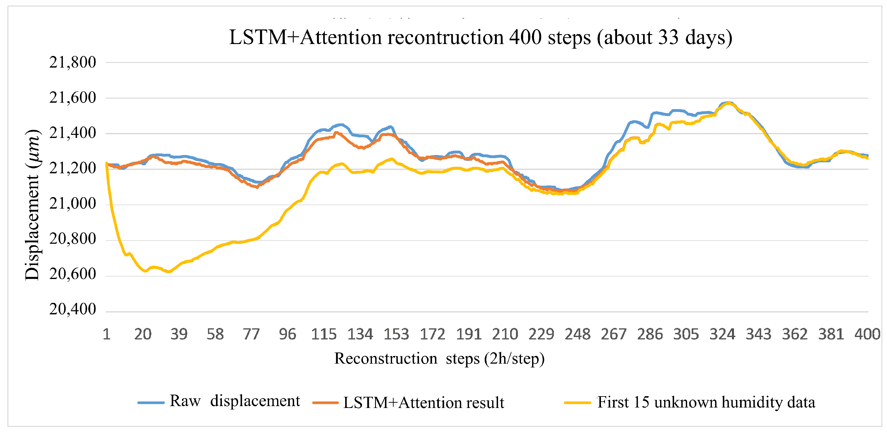
To verify the necessity of the environmental factors, this paper removes the current environmental data from the input data. The recent displacement data (unknown recent environmental data) is reconstructed based on the historical displacement and environmental data. The reconstruction results are compared with the known current environmental data for the experiment.
As observed in Figure 13, the LSTM-Attention model exhibits a significant reconstruction error when faced with unknown humidity conditions. The reconstruction error rapidly increases within the first 15 steps before gradually converging toward the actual value. This behavior suggests humidity plays a substantial role in the reconstruction process, particularly within the initial 15 steps. Initially, when the recent humidity remains unknown, the LSTM-Attention model lacks the necessary contextual information to reconstruct the data accurately, resulting in a significant reconstruction error. As the reconstruction progresses and the recent humidity becomes known, the influence of previous humidity values diminishes, leading to a gradual reduction in the reconstruction error. This observation underscores the criticality of the recent environmental factors for accurate displacement reconstruction in ancient buildings.

3.6. Ablation Study

Ablation experiments were conducted to assess the impact of the self-attention mechanism in the LSTM-Attention model on reconstruction performance. Multiple ablation experiments were conducted under the parameter settings of a time window length of 14 and a reconstruction step of 1. We conducted three experiments on both without attention mechanism and with attention mechanism. As presented in Table 7, when there is no attention mechanism, the MAE is 39.570, 37.391, 39.114, and RMSE is 52.530, 46.472, and 49.668, respectively. However, when there is an attention mechanism in the model, the MAE is 27.023, 27.293, and 26 863, RMSE is 37.239, 34.933, 35.287. This clearly shows that the performance of the model with an attention mechanism can be significantly improved, with an average improvement of 30.1% in MAE and 27.6% in RMSE. The results indicate that when the self-attention mechanism is absent in the LSTM network, the error is higher than when it is included. This finding suggests that the self-attention mechanism can help the model focus on more useful and critical information, effectively enhances the accuracy of the reconstruction, resulting in an average improvement of 15%. Therefore, the self-attention mechanism is deemed necessary and highly beneficial for anomaly detection in ancient buildings.

3.7. Model Comparison

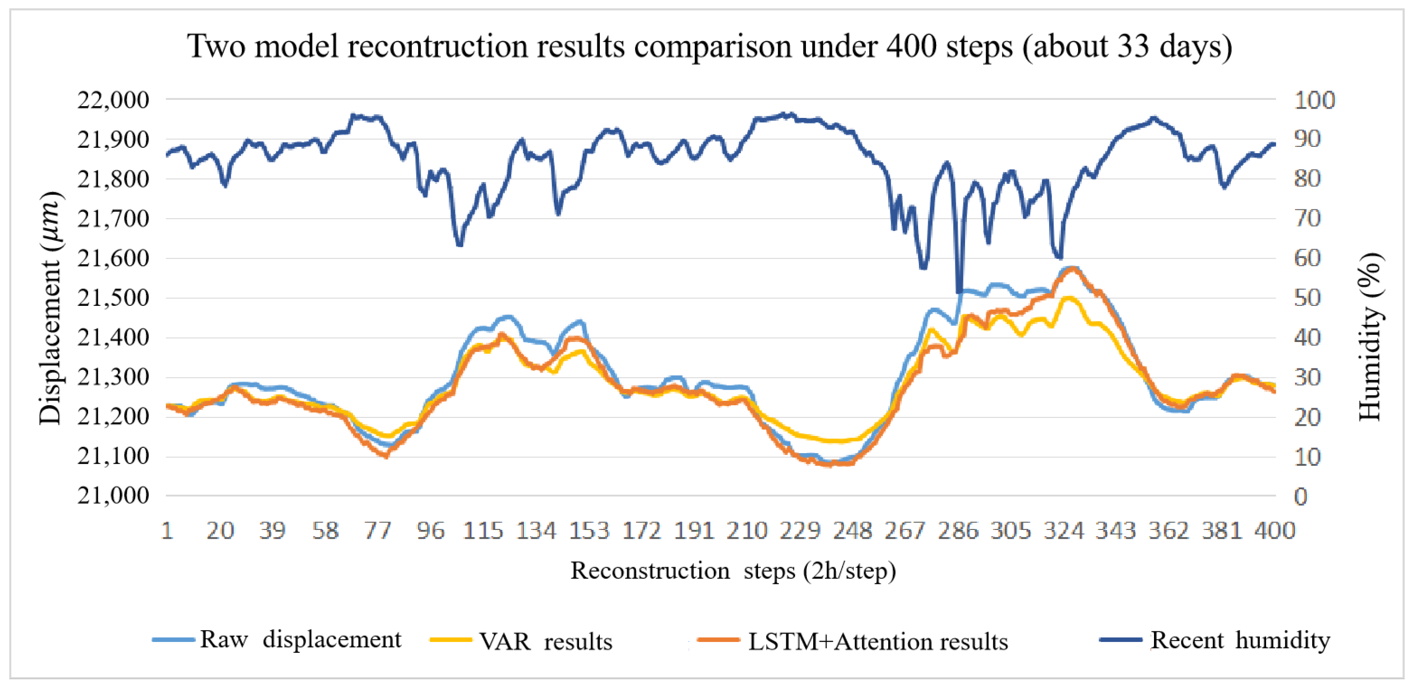
In machine learning, Vector Autoregression (VAR) [47] is a multi-variable time series prediction model that can assess the long-term lagged effects of environmental factors on ancient buildings. In prediction and anomaly detection tasks, VAR describes a linear relationship between variables, while LSTM, as a deep learning model, describes a nonlinear relationship between variables. Therefore, we represent VAR as a traditional method and LSTM-Attention as a deep learning approach and analyze them in detail. Figure 14 illustrates the reconstruction results of both models for a tenon displacement in the test set, indicating that both models can effectively reconstruct the tenon displacement when the humidity is known.
Performance metrics were computed across various reconstruction steps to facilitate a more intuitive comparison of the reconstruction capabilities between the two models. As illustrated in Figure 15, both MAE and RMSE exhibit an upward trend with increasing reconstruction steps. However, our framework consistently demonstrates lower values in these two metrics than in VAR. Even when reaching 400 reconstruction steps, the MAE and RMSE for our model remain confined within a specific range, typically below 30 μm and 40 μm, respectively. In contrast, VAR’s MAE and RMSE values are within a higher range, generally between 40 μm and 50 μm. This observation underscores the superior performance of our model over VAR. Furthermore, it is worth noting that while the number of reconstruction steps influences reconstruction error, its impact can still be effectively controlled within specific limits, primarily attributed to incorporating environmental factors.
Furthermore, a comparison was conducted to assess the performance of our proposed framework against several well-established baseline models, including the Autoregressive Integrated Moving Average Model (ARIMA) [48], Convolutional Neural Network (CNN) [49], and LSTM. The results of this comparison are summarized in Table 8, demonstrating the superior performance of our proposed model. Specifically, the MAE of ARIMA, VAR, CNN, and LSTM are 56.182, 38.950, 51.337, and 38.692, while the MAE of our model is 27.060. Compared to these alternative models, our proposed framework achieved remarkable MAE reductions of 51.9%, 30.5%, 47.3%, and 30.1%, respectively. The RMSE of ARIMA, VAR, CNN, LSTM, and our framework are 62.056, 44.721, 57.865, 47.751, and 34.328, and the RMSE of our model outperforms other baselines by 44.7%, 23.2%, 40.7%, and 28.1%, respectively.
Figure 16 visually represents the Receiver Operating Characteristic (ROC) curves of the models, with the corresponding Area Under the Curve (AUC) values marked in the figure. The larger the AUC value, the better the model performance. Notably, all AUC values of the five models exceed 0.5, signifying the models’ competence in anomaly detection. However, it is conspicuous that the AUC value for the LSTM-Attention model surpasses the rest of the four baseline models, asserting its prominence. Our model’s performance is also improved when compared with these baseline models, with AUC improvement of 15.4%, 3.8%, 3.6%, and 2.3%, which highlights the effectiveness of our model. Thus, our framework exhibits the most robust anomaly detection capability and higher accuracy, which means it excels in efficiently detecting anomalies within ancient buildings, thereby delivering heightened practical value.

3.8. Analysis of Anomaly Warning Indicators

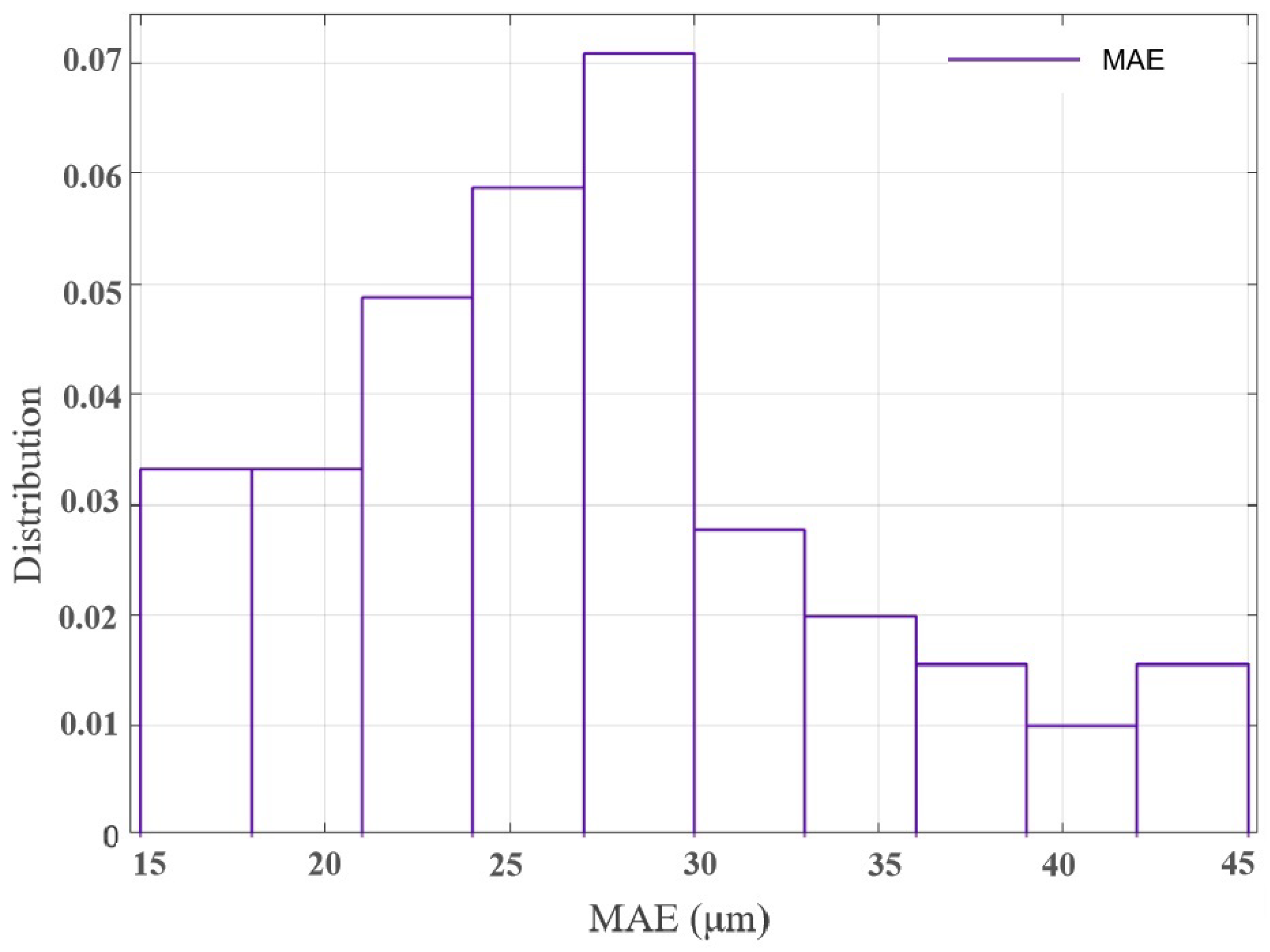
This paper utilizes the probability distribution of reconstruction errors to establish abnormal warning thresholds, which serve as warning indicators for different recurrence periods. Initially, probability statistics are conducted on the model’s reconstruction errors. Figure 17 illustrates the distribution probabilities of MAE, which predominantly cluster within the range of μm. Subsequently, a cumulative probability model is fitted to the data. Finally, anomaly warning thresholds are derived from the probabilistic model based on extreme recurrence intervals. Table 9 presents the anomaly warning thresholds of the LSTM-Attention model for 400 reconstruction steps, considering recurrence intervals of one and five years. Suppose the discrepancy between the reconstructed displacement and the actual value exceeds the anomaly warning threshold during monitoring. In that case, it indicates that the building has recently developed anomalous conditions and requires some protective measures.
This paper eventually deploys the anomaly warning for ancient buildings based on environmental constraints to practical engineering applications. Based on the probability distribution of the reconstruction error, the warning threshold under different recurrence intervals can be derived and used as the warning indicator. In Figure 12, it is demonstrated that the MAE of the 400-step reconstruction of the test set by the LSTM-Attention model can be stabilized within a certain range. The early warning indicator calculation process is divided into two steps:
  • Probabilistic statistics on MAE. The distribution probability of the error of the test set can be seen in Figure 17, which mainly focuses on the range of 25–30 μm, for which a cumulative probability model is fitted.
  • Extract the anomaly warning threshold from the probabilistic model based on the extreme recurrence intervals. Table 9 presents the anomaly warning thresholds of the LSTM-Attention model for 400 steps of reconstruction errors, considering recurrence intervals of one and five years.

4. Discussion

Our work is one of the few attempts to apply AI methods to ancient architecture conservation, tackling the anomaly detection challenge in ancient buildings. Historically, safeguarding ancient structures depended on analyzing deterioration causes, but this approach had limitations regarding research complexity and generalizability. Moreover, establishing early warning thresholds based on deterioration mechanisms was challenging, hampering the effective utilization of monitoring data for early anomaly detection in ancient buildings. To overcome these limitations, this paper introduces the application of artificial intelligence techniques, specifically the LSTM-Attention model, to offer real-time anomaly warnings for ancient buildings while considering environmental factors.
We did several experiments to analyze our model and compared with other common four models, when time step = 400, the MAE and RMSE are 27.060 and 34.328, respectively, which shows a large performance improvement compared with ARIMA, VAR, CNN, and LSTM, and the MAE is improved by 51.9%, 30.5%, 47.3%, and 30.1%, respectively. RMSE exceeds by 44.7%, 23.2%, 40.7%, and 28.1%. And in ROC, we have the largest AUC value. This suggests that our model is feasible in cultural protection anomaly detection. Furthermore, the proposed algorithm is implemented in practical engineering applications for the protection of real-life ancient architectural artifacts, providing valuable insights and applications for the preservation of ancient buildings worldwide.
However, the model exhibits certain limitations. It currently considers only temperature and humidity as influencing factors, overlooking crucial elements like acid rain, chemicals, and atmospheric conditions. Factors such as acid rain, chemicals, and atmospheric pollution can significantly accelerate the deterioration and destruction of ancient buildings. We utilize and install relevant sensors to collect other environmental data, analyze their impact on the structure of ancient buildings, and then model them to explore their correlations. Furthermore, to enhance our understanding and application of advanced algorithms for cultural artifacts, including Transformer [31], Autoformer [50], Informer [28], we are actively engaged in ongoing research and experimental work. Additionally, the current model lacks optimization algorithms, which can optimize the internal parameters of the model like the weights and thresholds, as well as external hyperparameters like the number of neurons, learning rate, and number of network layers, presenting an opportunity for future improvements in performance. Subsequent research endeavors will focus on incorporating additional influencing factors and developing suitable optimization algorithms to enhance the accuracy of the model.

5. Conclusions

Anomaly warning is of utmost importance in the realm of cultural heritage conservation. This study introduces an innovative anomaly warning methodology for ancient buildings operating under environmental constraints. We encompass the incorporation of seasonal, trend, shapelet, and mixed anomalies, augmenting both positive and negative samples, which enriches the detection range and improves the quality of model training. LSTM-Attention optimally captures intrinsic sequential relationships, enhancing the model’s capabilities. Our framework demonstrates the capability of multi-step anomaly detection by utilizing historical environmental data, tenon displacement data, and concurrent environmental data to reconstruct upcoming displacements. This capability allows flexibility in adjusting the time steps according to actual needs and helps to provide early warning of potential threats in ancient buildings. Anomaly threshold extraction is achieved by combining extreme value theory and recurrence interval calculation. In comparative analyses against four baselines, ARIMA, VAR, CNN, and LSTM, the LSTM-Attention model has higher accuracy and robustness for anomaly detection in ancient buildings. The RMSE and MAE metrics of the LSTM-Attention model are significantly improved, and the AUC value is the highest, which proves that the LSTM-Attention model has higher efficacy and applicability in monitoring ancient buildings. Ablation experiments further confirmed the contribution of the attention mechanism. Surprisingly, we have deployed several servers at the experimental base and designed an IoT platform system; thus, the early warning algorithm in this paper has achieved a smooth landing without worrying about computational resources, and applied to real-world scenarios to satisfy the needs of non-development enterprises, proving its universality and practicality in heritage conservation. This work is poised to promote the development of cutting-edge technologies and methods for ancient building conservation.
In our next work, we will focus on the following aspects: (1) In this study, our investigation was confined to the influence of humidity and temperature on ancient buildings. Therefore, an expanded exploration of other factors is necessary. (2) The anomaly warning is based on reconstruction error, sequence difference [51] is also a commonly used method that can be considered in the future. (3) Model performance can be further improved by integrating optimization algorithms. For instance, the heuristic algorithms [52,53] could facilitate the refinement of model parameters to improve reconstruction ability. (4) Notably, this study is an initial attempt to employ deep learning techniques for anomaly detection in cultural heritage. As the study progresses, we will explore more methods applicable to cultural heritages.

Author Contributions

Conceptualization, Y.W. and Z.S.; methodology, Y.W. and X.M.; software, Z.S.; validation, Y.W. and Z.S.; formal analysis, Y.W. and X.M.; investigation, Y.W. and Z.S.; resources, Z.S.; data curation, Z.S.; writing—original draft preparation, Y.W.; writing—review and editing, X.M. and Y.H.; visualization, Y.W. and Z.S.; supervision, Y.D., P.J. and D.L. project administration, Y.D. and P.J.; funding acquisition, Y.D. and P.J. All authors have read and agreed to the published version of the manuscript.

Funding

This work was supported by the Ningbo Public Welfare Project on “Research and Demonstration of Early Warning Method for Abnormal Structural Changes of Ancient Buildings Based on Normal Model” (No. 2022S172). Science and Technology Program of Zhejiang Province (No. 2023C03183).

Data Availability Statement

The data can be shared upon request.

Acknowledgments

The authors would like to thank the editor and reviewers for their valuable time and suggestions to improve the quality of the manuscript.

Conflicts of Interest

Author Ping Jia was employed by the company China Mobile Group Zhejiang Company Limited. The remaining authors declare that the research was conducted in the absence of any commercial or financial relationships that could be construed as a potential conflict of interest.

References

  1. Qu, J.J.; Cheng, G.D.; Zhang, K.C.; Wang, J.C.; Zu, R.P.; Fang, H.Y. An experimental study of the mechanisms of freeze/thaw and wind erosion of ancient adobe buildings in northwest China. Bull. Eng. Geol. Environ. 2007, 66, 153–159. [Google Scholar] [CrossRef]
  2. Betti, M.; Galano, L.; Vignoli, A. Finite element modelling for seismic assessment of historic masonry buildings. Earthquakes and Their Impact on Society; Springer: Cham, Switzerland, 2016; pp. 377–415. [Google Scholar]
  3. Ereiz, S.; Duvnjak, I.; Damjanović, D.; Bartolac, M. Analysis of seismic action on the tie rod system in historic buildings using finite element model updating. Buildings 2021, 11, 453. [Google Scholar] [CrossRef]
  4. Liu, S.; Wang, R.; Yu, J.; Peng, X.; Cai, Y.; Tu, B. Effectiveness of the anti-erosion of an MICP coating on the surfaces of ancient clay roof tiles. Constr. Build. Mater. 2020, 243, 118202. [Google Scholar] [CrossRef]
  5. Xin, Z.; Ke, D.; Zhang, H.; Yu, Y.; Liu, F. Non-destructive evaluating the density and mechanical properties of ancient timber members based on machine learning approach. Constr. Build. Mater. 2022, 341, 127855. [Google Scholar] [CrossRef]
  6. Tao, S. Protection and repair technology of ancient building walls based on big data. In Civil Engineering and Urban Research; CRC Press: Boca Raton, FL, USA, 2023; Volume 1, pp. 311–317. [Google Scholar]
  7. Akcaozoglu, S.; Yavascan, E.E.; Gokce, M.V. Deterioration and Conservation Problems of Historical Fountains in Cappadocia-Niğde. Fresenius Environ. Bull. 2020, 29, 2338–2343. [Google Scholar]
  8. Hatır, M.E.; İnce, İ.; Korkanç, M. Intelligent detection of deterioration in cultural stone heritage. J. Build. Eng. 2021, 44, 102690. [Google Scholar] [CrossRef]
  9. Severcan, M.H.; Yavaşcan, E.E.; Akçaözoğlu, S.; Akçaözoğlu, K. Investigation of material deterioration and seismic behavior of Fertek and Hançerli Churches in Cappadocia Region. Niğde Ömer Halisdemir Üniversitesi Mühendislik Bilim. Derg. 2022, 11, 1042–1052. [Google Scholar]
  10. Liu, X.; Koestler, R.J.; Warscheid, T.; Katayama, Y.; Gu, J.D. Microbial deterioration and sustainable conservation of stone monuments and buildings. Nat. Sustain. 2020, 3, 991–1004. [Google Scholar] [CrossRef]
  11. Fanti, R.; Gigli, G.; Tapete, D.; Mugnai, F.; Casagli, N. Monitoring and modelling slope instability in cultural heritage sites. In Landslide Science and Practice; Volume 6: Risk Assessment, Management and Mitigation; Springer: Berlin/Heidelberg, Germany, 2013; pp. 467–473. [Google Scholar]
  12. Holickỳ, M.; Sỳkora, M. Assessment of flooding risk to cultural heritage in historic sites. J. Perform. Constr. Facil. 2010, 24, 432–438. [Google Scholar] [CrossRef]
  13. Staley, D.M.; Negri, J.A.; Kean, J.W.; Laber, J.L.; Tillery, A.C.; Youberg, A.M. Prediction of spatially explicit rainfall intensity–duration thresholds for post-fire debris-flow generation in the western United States. Geomorphology 2017, 278, 149–162. [Google Scholar] [CrossRef]
  14. Liang, H.; Zou, J.; Khan, M.J.; Jinxuan, H. An sand plug of fracturing intelligent early warning model embedded in remote monitoring system. IEEE Access 2019, 7, 47944–47954. [Google Scholar] [CrossRef]
  15. Gigli, G.; Fanti, R.; Canuti, P.; Casagli, N. Integration of advanced monitoring and numerical modeling techniques for the complete risk scenario analysis of rockslides: The case of Mt. Beni (Florence, Italy). Eng. Geol. 2011, 120, 48–59. [Google Scholar] [CrossRef]
  16. Xie, P.; Zhou, A.; Chai, B. The application of long short-term memory (LSTM) method on displacement prediction of multifactor induced landslides. IEEE Access 2019, 7, 54305–54311. [Google Scholar] [CrossRef]
  17. Fan, L.; Li, J.; Pan, Y.; Wang, S.; Yan, C.; Yao, D. Research and application of smart grid early warning decision platform based on big data analysis. In Proceedings of the 2019 4th International Conference on Intelligent Green Building and Smart Grid (IGBSG), Hubei, China, 6–9 September 2019; pp. 645–648. [Google Scholar]
  18. Zhu, X.; Jin, X.; Jia, D.; Sun, N.; Wang, P. Application of data mining in an intelligent early warning system for rock bursts. Processes 2019, 7, 55. [Google Scholar] [CrossRef]
  19. Chen, Z.; Chen, D.; Zhang, X.; Yuan, Z.; Cheng, X. Learning graph structures with transformer for multivariate time-series anomaly detection in IoT. IEEE Internet Things J. 2021, 9, 9179–9189. [Google Scholar] [CrossRef]
  20. Shah, G.; Tiwari, A. Anomaly detection in iiot: A case study using machine learning. In Proceedings of the ACM India Joint International Conference on Data Science and Management of Data, Goa, India, 11–13 January 2018; pp. 295–300. [Google Scholar]
  21. Feng, X.; Song, D.; Chen, Y.; Chen, Z.; Ni, J.; Chen, H. Convolutional transformer based dual discriminator generative adversarial networks for video anomaly detection. In Proceedings of the 29th ACM International Conference on Multimedia, Virtual Event, China, 20–24 October 2021; pp. 5546–5554. [Google Scholar]
  22. Bhuvaneshwari, P.; Rao, A.N.; Robinson, Y.H.; Thippeswamy, M. Sentiment analysis for user reviews using Bi-LSTM self-attention based CNN model. Multimed. Tools Appl. 2022, 81, 12405–12419. [Google Scholar] [CrossRef]
  23. Li, J.; Zhang, Z.; Lang, J.; Jiang, Y.; An, L.; Zou, P.; Xu, Y.; Gao, S.; Lin, J.; Fan, C.; et al. Hybrid multimodal feature extraction, mining and fusion for sentiment analysis. In Proceedings of the 3rd International on Multimodal Sentiment Analysis Workshop and Challenge, Lisboa, Portugal, 10 October 2022; pp. 81–88. [Google Scholar]
  24. Fan, Z.; Hu, G.; Sun, X.; Wang, G.; Dong, J.; Su, C. Self-attention neural architecture search for semantic image segmentation. Knowl.-Based Syst. 2022, 239, 107968. [Google Scholar] [CrossRef]
  25. Li, K.; Qian, Z.; Han, Y.; Eric, I.; Chang, C.; Wei, B.; Lai, M.; Liao, J.; Fan, Y.; Xu, Y. Weakly supervised histopathology image segmentation with self-attention. Med. Image Anal. 2023, 86, 102791. [Google Scholar] [CrossRef]
  26. Fan, Z.; Liu, Z.; Wang, Y.; Wang, A.; Nazari, Z.; Zheng, L.; Peng, H.; Yu, P.S. Sequential recommendation via stochastic self-attention. In Proceedings of the ACM Web Conference 2022, Virtual Event, Lyon, France, 25–29 April 2022; pp. 2036–2047. [Google Scholar]
  27. Zhang, Y.; Yang, B.; Liu, H.; Li, D. A time-aware self-attention based neural network model for sequential recommendation. Appl. Soft Comput. 2023, 133, 109894. [Google Scholar] [CrossRef]
  28. Zhou, H.; Zhang, S.; Peng, J.; Zhang, S.; Li, J.; Xiong, H.; Zhang, W. Informer: Beyond efficient transformer for long sequence time-series forecasting. In Proceedings of the AAAI Conference on Artificial Intelligence; Association for the Advancement of Artificial Intelligence: Washington, DC, USA, 2021; Volume 35, pp. 11106–11115. [Google Scholar]
  29. Chen, M.; Peng, H.; Fu, J.; Ling, H. Autoformer: Searching transformers for visual recognition. In Proceedings of the IEEE/CVF International Conference on Computer Vision, Montreal, BC, Canada, 11–17 October 2021; pp. 12270–12280. [Google Scholar]
  30. Hu, Y.; Xiao, F. Network self attention for forecasting time series. Appl. Soft Comput. 2022, 124, 109092. [Google Scholar] [CrossRef]
  31. Vaswani, A.; Shazeer, N.; Parmar, N.; Uszkoreit, J.; Jones, L.; Gomez, A.N.; Kaiser, Ł.; Polosukhin, I. Attention is all you need. Adv. Neural Inf. Process. Syst. 2017, 30. [Google Scholar]
  32. Hochreiter, S.; Schmidhuber, J. Long short-term memory. Neural Comput. 1997, 9, 1735–1780. [Google Scholar] [CrossRef] [PubMed]
  33. Chang, T.A.; Bergen, B.K. Word acquisition in neural language models. Trans. Assoc. Comput. Linguist. 2022, 10, 1–16. [Google Scholar] [CrossRef]
  34. Oota, S.R.; Alexandre, F.; Hinaut, X. Long-term plausibility of language models and neural dynamics during narrative listening. In Proceedings of the Annual Meeting of the Cognitive Science Society; Cognitive Science Society: Seattle, WA, USA, 2022; Volume 44. [Google Scholar]
  35. Kumar, R.; Kumar, P.; Kumar, Y. Three stage fusion for effective time series forecasting using Bi-LSTM-ARIMA and improved DE-ABC algorithm. Neural Comput. Appl. 2022, 34, 18421–18437. [Google Scholar] [CrossRef]
  36. Wang, H.; Zhang, Y.; Liang, J.; Liu, L. DAFA-BiLSTM: Deep Autoregression Feature Augmented Bidirectional LSTM network for time series prediction. Neural Netw. 2023, 157, 240–256. [Google Scholar] [CrossRef] [PubMed]
  37. Bhaskar, S.; Thasleema, T. LSTM model for visual speech recognition through facial expressions. Multimed. Tools Appl. 2023, 82, 5455–5472. [Google Scholar] [CrossRef]
  38. Premalatha, S.; Kumar, V.; Jagini, N.P.; Reddy, G.V.S. Development of vanilla LSTM based stuttered speech recognition system using bald eagle search algorithm. Signal, Image Video Process. 2023, 17, 4077–4086. [Google Scholar] [CrossRef]
  39. Wu, Y.; Sun, L.; Sun, X.; Wang, B. A hybrid XGBoost-ISSA-LSTM model for accurate short-term and long-term dissolved oxygen prediction in ponds. Environ. Sci. Pollut. Res. 2022, 29, 18142–18159. [Google Scholar] [CrossRef]
  40. Li, Y.; Zhu, Z.; Kong, D.; Han, H.; Zhao, Y. EA-LSTM: Evolutionary attention-based LSTM for time series prediction. Knowl.-Based Syst. 2019, 181, 104785. [Google Scholar] [CrossRef]
  41. Liu, X.; Shi, R.; Hui, Q.; Xu, S.; Wang, S.; Na, R.; Sun, Y.; Ding, W.; Zheng, D.; Chen, X. TCACNet: Temporal and channel attention convolutional network for motor imagery classification of EEG-based BCI. Inf. Process. Manag. 2022, 59, 103001. [Google Scholar] [CrossRef]
  42. Kim, H.; Kim, S.; Shin, H.; Heo, J.H. Appropriate Model Selection Methods for Nonstationary Generalized Extreme Value Models. J. Hydrol. 2017, 547, 557–574. [Google Scholar] [CrossRef]
  43. Martins, E.; Stedinger, J. Generalized Maximum Likelihood GEV Quantile Estimators for Hydrologic Data. Water Resour. Res. 2000, 36, 737–744. [Google Scholar] [CrossRef]
  44. Chikobvu, D.; Chifurira, R. Modelling of extreme minimum rainfall using generalised extreme value distribution for Zimbabwe. South Afr. J. Sci. 2015, 111, 1–8. [Google Scholar] [CrossRef]
  45. Calabrese, R.; Giudici, P. Estimating bank default with generalised extreme value regression models. J. Oper. Res. Soc. 2015, 66, 1783–1792. [Google Scholar] [CrossRef]
  46. Rocco, M. Extreme Value Theory for Finance: A Survey. J. Econ. Surv. 2012, 28. [Google Scholar] [CrossRef]
  47. Johansen, S. Modelling of cointegration in the vector autoregressive model. Econ. Model. 2000, 17, 359–373. [Google Scholar] [CrossRef]
  48. Box, G.E.; Pierce, D.A. Distribution of residual autocorrelations in autoregressive-integrated moving average time series models. J. Am. Stat. Assoc. 1970, 65, 1509–1526. [Google Scholar] [CrossRef]
  49. LeCun, Y.; Bottou, L.; Bengio, Y.; Haffner, P. Gradient-based learning applied to document recognition. Proc. IEEE 1998, 86, 2278–2324. [Google Scholar] [CrossRef]
  50. Wu, H.; Xu, J.; Wang, J.; Long, M. Autoformer: Decomposition transformers with auto-correlation for long-term series forecasting. Adv. Neural Inf. Process. Syst. 2021, 34, 22419–22430. [Google Scholar]
  51. Zhao, C.; Chang, X.; Xie, T.; Fujita, H.; Wu, J. Unsupervised anomaly detection based method of risk evaluation for road traffic accident. Appl. Intell. 2023, 53, 369–384. [Google Scholar] [CrossRef]
  52. Tayarani-N, M.H.; Yao, X.; Xu, H. Meta-heuristic algorithms in car engine design: A literature survey. IEEE Trans. Evol. Comput. 2014, 19, 609–629. [Google Scholar] [CrossRef]
  53. Naruei, I.; Keynia, F. Wild horse optimizer: A new meta-heuristic algorithm for solving engineering optimization problems. Eng. Comput. 2022, 38, 3025–3056. [Google Scholar] [CrossRef]
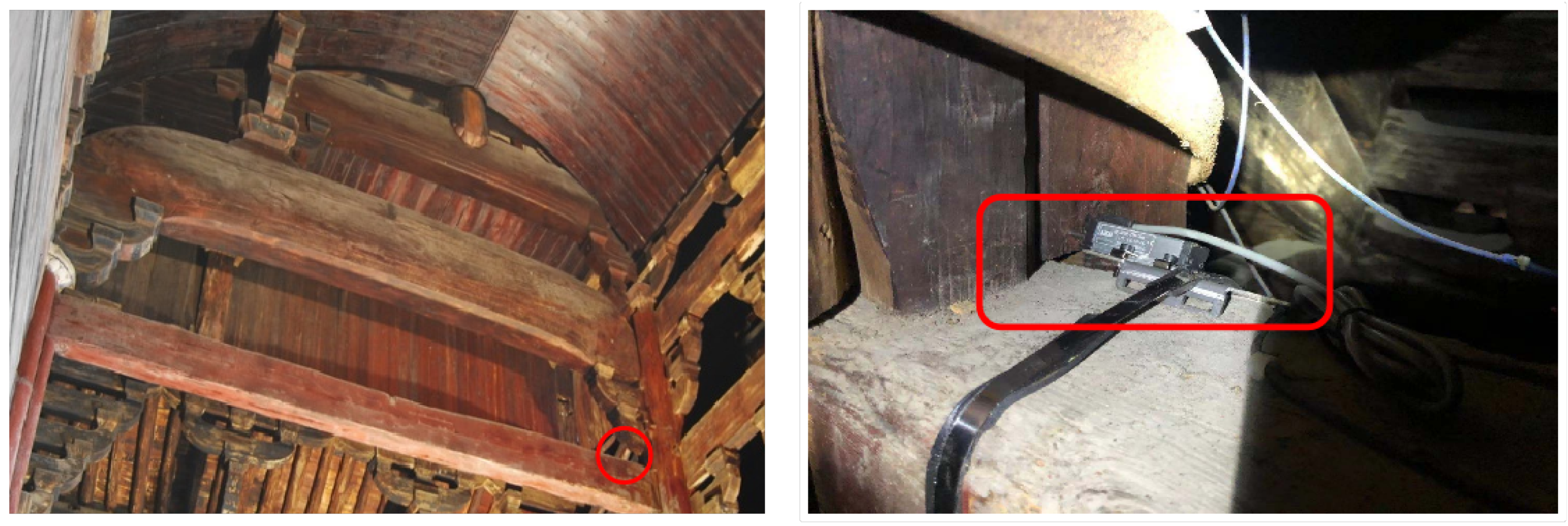
Figure 1. Installation point of tenon displacement sensor. The sensor mounting position is marked in the picture with a red circle and a red box to make it clearly visible.
Electronics 13 01254 g001
Figure 2. Data synthesis.
Electronics 13 01254 g002
Figure 3. Attention.
Electronics 13 01254 g003
Figure 4. The basic LSTM cell.
Electronics 13 01254 g004
Figure 5. The LSTM-Attention model.
Electronics 13 01254 g005
Figure 6. Scatter plots between two environmental factors and the tenon displacement.
Electronics 13 01254 g006
Figure 7. Preprocessing data results.
Electronics 13 01254 g007
Figure 8. Influence coefficient a and MAE corresponding to different lag time d.
Electronics 13 01254 g008
Figure 9. Metrics indexes under different time window lengths.
Electronics 13 01254 g009
Figure 10. Metrics indexes under different reconstruction steps.
Electronics 13 01254 g010
Figure 11. Performance comparison of LSTM-Attention with different parameters.
Electronics 13 01254 g011
Figure 12. Reconstruction error of LSTM-Attention model.
Electronics 13 01254 g012
Figure 13. Comparison of reconstruction results of the LSTM-Attention model in the case of known/unknown humidity.
Electronics 13 01254 g013
Figure 14. Comparison of reconstruction results of the LSTM-Attention model in the case of known/unknown humidity.
Electronics 13 01254 g014
Figure 15. Comparison of VAR and LSTM-Attention under different reconstruction steps.
Electronics 13 01254 g015
Figure 16. ROC curves for anomaly detection.
Electronics 13 01254 g016
Figure 17. MAE probability distribution graph.
Electronics 13 01254 g017
Table 1. Part of the original data.
TimeDisplacement (μm)Temperature (°C)Humidity (%)
00:00:0021,321.525.43898.175
02:00:0021,32025.66197.938
04:00:0021,318.525.96797.228
06:00:0021,316.7526.28296.248
20:00:0021,311.523.17396.108
22:00:0021,308.2522.87095.871
Table 2. Parameters related to anomalies.
ParameterValue
α 0.2
β 0.005
γ 0.2
ω 24
ω ^ 48
Table 3. ROC definition table.
Reference
PositiveNegative
PredictionPositiveTP (True Positive)FP (False Positive)
NegativeFN (False Negative)TN (True Negative)
Table 4. Performance comparison with different α .
Metrics0.050.10.20.30.4
MAE36.13938.36127.0628.23734.475
RMSE35.54936.13434.32836.49742.573
Table 5. Performance comparison with different β .
Metrics0.050.10.20.30.4
MAE34.93129.04827.0629.87331.462
RMSE39.02740.08434.32841.34932.274
Table 6. Performance comparison with different γ .
Metrics0.0010.0050.010.020.03
MAE30.47827.0631.57832.86231.847
RMSE32.13834.32835.74536.59735.864
Table 7. Results of ablation experiments.
Evaluation MetricsWithout Attention MechanismWith Attention Mechanism
MAE39.57027.023
37.39127.293
39.11426.863
RMSE52.53037.239
46.47234.933
49.66835.287
Table 8. Performance comparison of five models (400 steps).
ModelMAERMSE
ARIMA56.18262.056
VAR38.95044.721
CNN51.33757.865
LSTM38.69247.751
LSTM-Attention27.06034.328
Table 9. Anomaly warning thresholds at different recurrence intervals.
Recurrence IntervalMAE
One year70.3789
Five years75.1033
Disclaimer/Publisher’s Note: The statements, opinions and data contained in all publications are solely those of the individual author(s) and contributor(s) and not of MDPI and/or the editor(s). MDPI and/or the editor(s) disclaim responsibility for any injury to people or property resulting from any ideas, methods, instructions or products referred to in the content.