An Efficient Multi-Scale Attention Feature Fusion Network for 4K Video Frame Interpolation

Abstract

Video frame interpolation aims to generate intermediate frames in a video to showcase finer details. However, most methods are only trained and tested on low-resolution datasets, lacking research on 4K video frame interpolation problems. This limitation makes it challenging to handle high-frame-rate video processing in real-world scenarios. In this paper, we propose a 4K video dataset at 120 fps, named UHD4K120FPS, which contains large motion. We also propose a novel framework for solving the 4K video frame interpolation task, based on a multi-scale pyramid network structure. We introduce self-attention to capture long-range dependencies and self-similarities in pixel space, which overcomes the limitations of convolutional operations. To reduce computational cost, we use a simple mapping-based approach to lighten self-attention, while still allowing for content-aware aggregation weights. Through extensive quantitative and qualitative experiments, we demonstrate the excellent performance achieved by our proposed model on the UHD4K120FPS dataset, as well as illustrate the effectiveness of our method for 4K video frame interpolation. In addition, we evaluate the robustness of the model on low-resolution benchmark datasets.

1. Introduction

Video frame interpolation (VFI) is a widely used technique to increase the frame rate of video by synthesising intermediate frames between given consecutive frames, resulting in smoother video playback with reduced motion blur and jitter. This technique has been applied extensively in various applications, such as slow motion generation [1], video restoration [2], video compression [3], and novel view synthesis [4]. However, the optimisation of the deep learning-based VFI method is mainly limited to low-resolution benchmark datasets, which cannot be generalised to higher-resolution video (e.g., 4K or 8K), as shown in Figure 1. 4K video contains more spatial information and extreme pixel displacement, increasing motion blur and jitter, and posing greater challenges for the VFI method to interpolate frames accurately. Furthermore, the CNN-based [5,6] VFI method has limited ability to capture long-range dependencies and model non-local self-similarity, leading to difficulties in handling larger motions.

In order to address the above challenges in VFI, we propose a novel high-quality 4K video dataset called UHD4K120FPS, which consists of a wide range of realistic scenes with high resolution (HR), high frame rate (HFR), and high dynamic range (HDR) features. As shown in Figure 2, the average maximum brightness value of the samples is around 200% under BT.2020. This indirectly demonstrates that our dataset contains large motion and complex texture information.

Meanwhile, we propose an efficient 4K VFI model that learns large-scale features. Our model uses a pyramid network to extract multi-scale information from 4K frames and employs self-attention in Transformers [10] to model long-range pixel correlation among frames. To address convolutional operation locality on large-scale feature maps, we redesign self-attention and perform simple mapping on input feature maps. By mapping query, key, and value using multiple 1 × 1 convolutions, we reduce model complexity. Multi-head self-attention calculates the mapped query, key, and value while enhancing the output of self-attention through convolutional operations. In encoding, we extract contextual information from feature maps at different scales to capture motion detail in 4K frames. Meanwhile, in decoding, we fuse the feature maps of different scales as the output of the pyramid.

In summary, our main contributions are as follows:

• We propose a novel VFI framework based on multi-scale attention feature fusion network for 4K VFI tasks.
• We propose the UHD4K120FPS dataset, a high-quality 4K video dataset at 120 fps, containing diverse texture information and large motion, which can be used for 4K VFI tasks.
• Our method effectively captures the long-range pixel dependence and self-similarity in 4K frames, while reducing the computational cost of attention through simple mapping. It performs well on the UHD4K120FPS dataset and multiple benchmarks.

2. Related Work

Previous work in deep learning-based VFI can be divided into two types: flow-based and kernel-based methods.

2.1. Flow-Based

These methods predict optical flow to warp pixels and synthesise intermediate frames. Liu et al. [11] directly estimate intermediate flow from input frames for frame synthesis. Niklaus et al. [1] generate output frames by warping frames with bidirectional flow and utilising contextual information through deformable GridNet. To address the computational cost, Huang et al. [12] design a fast interpolation model, RIFE, which is 4–27 times faster than Super-SloMo [13] and DAIN [14]. Kong et al. [15] introduce IFRNet, a neural network based on a feature pyramid structure that estimates intermediate flow in real-time from coarse to fine and employs privileged distillation for training. Although these methods achieve good results, the accuracy of flow estimation significantly affects the quality of the generated frame.

2.2. Kernel-Based

To solve the problem of inaccurate optical flow estimation, kernel-based methods [7,8,16,17] generate new frames by convolving local patches and use CNN to estimate spatially adaptive convolution kernels. Niklaus et al. [16,17] proposed AdaConv and SepConv that use a convolutional network to estimate the adaptive convolution kernel for each pixel, and convolves the input frames with the predicted kernels to generate intermediate frames. However, the inflexibility of kernel shape limits the types of motion that such methods can handle. To overcome this limitation, Lee et al. [7] proposed the AdaCoF model based on adaptive flow collaboration, which uses deformable convolution kernels [18]. Similarly, Cheng et al. [19] proposed EDSC, which extends kernel-based VFI methods using deformable separable convolution. Additionally, Bao et al. [14] proposed an adaptive warping layer that combines flow-based and kernel-based methods to warp frames or features using the given optical flow and learned local convolution kernels. However, dealing with large motion often requires larger kernel sizes, leading to increased model parameters.

3. UHD4K120FPS Dataset

Currently, various benchmark datasets, such as Vimeo90K [9], UCF101 [20], and Middlebury [21], have been made available for VFI tasks. However, these datasets lack high-quality 4K videos with rich, high frame rates, which impedes the development of refined VFI methods for UHD videos. Recently, some 4K datasets have been used for VFI tasks, such as X4K1000FPS [5] and FISR [22]. However, these datasets have fewer data samples and are not suitable for our task.

We created an Ultra-high-definition (UHD) video dataset, named UHD4K120FPS, which comprises 300 high-dynamic-range video scenes captured in real-world environments using a SONY Alpha 1 digital camera (manufactured by Sony Corporation, Tokyo, Japan). Each scene has a spatial resolution of 3840 × 2160 and a frame rate of 120 fps, with durations ranging from 5 to 20 s. To ensure the selection of valuable data samples, we manually excluded blurry video scenes and selected 245 video clips, each with 5 consecutive frames, featuring various objects and scenes. We used GMFlowNet [23] to estimate bidirectional optical flows between the first and last frames in each video clips, and clips with small motion magnitude were eliminated by setting a threshold of 9 for the optical flow magnitudes of each clip. Ultimately, we selected 120 scenes with optical flow magnitudes ranging from 9.96 to 63.52 pixels, with an average of 17.97 pixels. Among these, 108 scenes were used as the training dataset, and 12 different scenes served as the testing dataset, denoted as ${\mathrm{UHD}}_{\mathrm{Text}}$, with each scene serving as a separate test sample. The average optical flow magnitudes of the test samples were 23.05 pixels, indicating the presence of large motion. The training dataset is denoted as ${\mathrm{UHD}}_{\mathrm{Train}}$. To create a training sample, we randomly cropped a series of 128 × 128 patches at the same location in 5 consecutive frames.

4. Proposed Method

This section specifically describes the implementation details of our proposed method. The goal of VFI is to synthesise an intermediate frame $I_t$ $(0<t<1)$ from two input frames $I_0$ and $I_1$. In this paper, we set $t=0.5$, that is, synthesising the middle frame between $I_0$ and $I_1$. Firstly, we describe the overall structure of our model, which consists of a Multi-scale Pyramid Network (MPNet), a Context Extraction Module (CEModule), and a Deformable Convolutional Synthesis Module (DConv SynModule), as shown in Figure 3.

Firstly, $I_0$ and $I_1$ are preprocessed, and then multi-scale feature map $F_t^{out}$, occlusion map M, and contextual feature maps $C_t^{0\sim 3}$ are obtained by MPNet and CEModule, respectively. DConv SynModule is applied to $F_t^{out}$ and $C_t^{0\sim 3}$ to generate warped frames $I_t^1$ and $I_t^2$, respectively. $I_t^1$, $I_t^2$, and M are combined using tensor operations to synthesise $I_t$. M is used to blend the two warped frames $I_t^1$ and $I_t^2$. $I_t$ is defined as:

$$I_t=M\odot I_t^1+(1-M)\odot I_t^2.$$

(1)

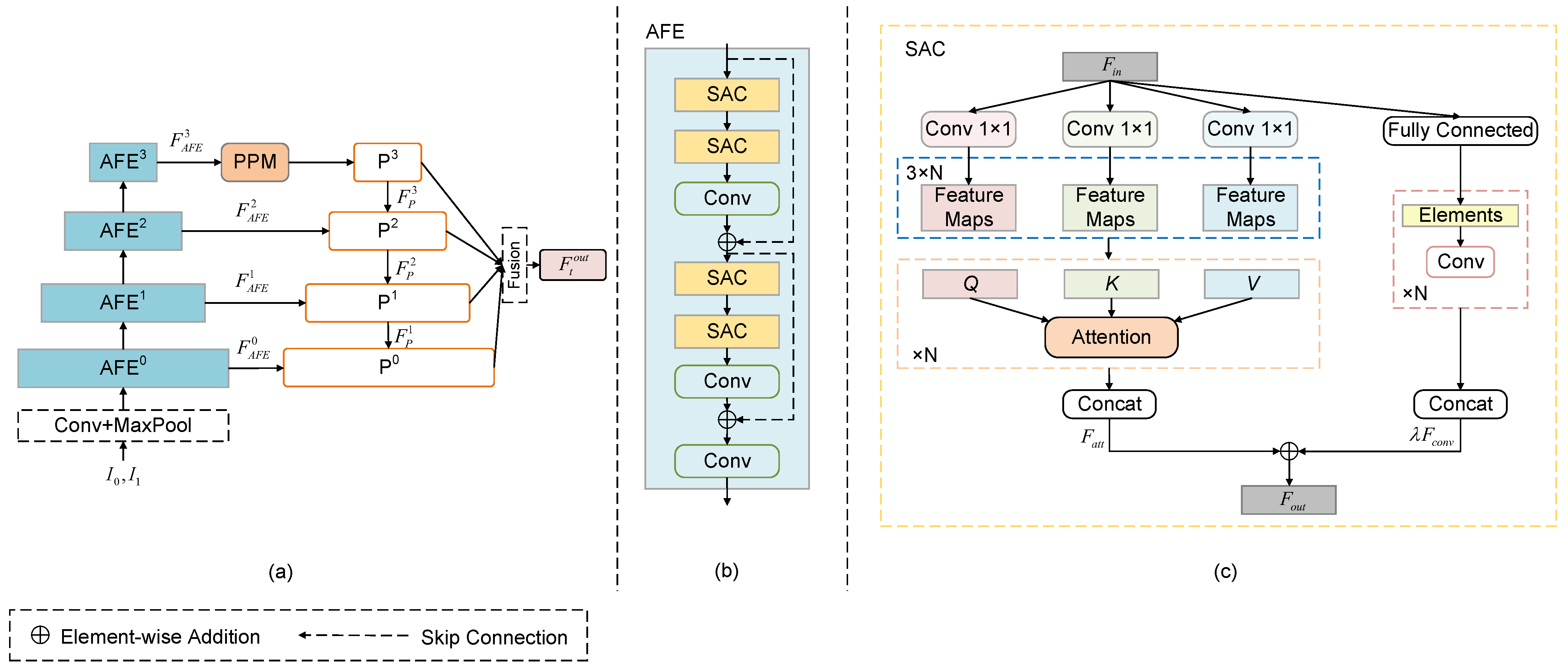
4.1. Multi-Scale Pyramid Network

We use a multi-scale pyramid network as an encoder–decoder framework, as shown in Figure 4a. The encoder (bottom-up) consists of 4 attention feature extraction (AFE) blocks, each with two residual blocks and a convolutional layer. Each residual block consists of two SAC blocks and a convolutional layer. The feature maps generated by AFEⁱ at different scales are denoted as $F_{AFE}^i$. The decoder (top-down) layers are composed of convolutional and upsampling layers, represented as Pⁱ. Applying the pyramid pooling module (PPM) [24] to $F_{AFE}^3$ generates P³’s output $F_P^3$, which is then upsampled and merged with $F_{AFE}^2$ through element-wise addition to generate $F_P^2$, and so on. Finally, $F_P^3$, $F_P^2$, and $F_P^1$ are upsampled and fused with $F_P^0$ to obtain $F_t^{out}$. Moreover, $F_t^{out}$ is used to estimate the occlusion map M.

4.2. Self-Attention Conv Module

Traditional CNNs struggle to model the semantic features of all pixels in single-frame images of high-resolution videos. To address this issue, we propose a novel module called SAC which captures long-range dependencies among pixels and models their semantics, as shown in Figure 4c. It employs the standard multi-head self-attention represented as a self-attention module with N heads. The input and output feature maps are represented by tensors $F_{in}\in {\mathbb{R}}^{H\times W\times C}$ and $F_{out}\in {\mathbb{R}}^{H\times W\times C}$, respectively, with their height, width, and number of channels denoted by H, W, and C. For the corresponding pixel $p(i,j)$, the input tensor is represented by $f_{ij}^{in}\in {\mathbb{R}}^C$, and the output tensor is represented by $f_{ij}^{out}\in {\mathbb{R}}^C$. The calculation process for the query Q, the key K, and the value V is as follows:

$$Q_{ij}^m=W_{\mathcal{Q}}^m{f}_{ij}^{in}, K_{ij}^m=W_K^m{f}_{ij}^{in}, V_{ij}^m=W_V^m{f}_{ij}^{in}$$

(2)

The weight matrices for Q, K, and V are denoted as $W_{\mathcal{Q}}^m$, $W_K^m$, and $W_{\mathcal{V}}^m$, respectively. Equation (2) reveals that the computation complexity of self-attention is predominantly concentrated in mapping Q, K, and V. To address this issue, we are inspired by paper [25]. We employ a simple mapping method that splits the self-attention computation into two stages. Initially, the input feature map is projected through three 1 × 1 convolutions, producing three sets of intermediate features, each containing N feature blocks. Subsequently, we sequentially traverse these three groups of intermediate features and partition them into N sets, with each set consisting of three feature blocks (corresponding to the three 1 × 1 convolutions) that are used for Q, K, and V computation. The second stage involves the calculation of $F_{att}$ based on multi-head self-attention, with the following equation:

$$\mathrm{Attention}(Q_{ij}^m,K_{ab}^m,V_{ab}^m)=\mathrm{softmax}\left(\frac{Q_{ij}^m{\left(K_{ab}^m\right)}^{\mathrm{T}}}{\sqrt{d}}\right)V_{ab}^m$$

(3)

$$f_{ij}^{out}=\stackrel{N}{\underset{m=1}{\mathrm{Concat}}}\left(\sum _{a,b\in X}\mathrm{Attention}(Q_{ij}^m,K_{ab}^m,V_{ab}^m)\right)$$

(4)

The dimension of the $Q_{ij}^m$ feature is denoted as d and X refers to the local region centered at $p(i,j)$. To enhance the ability of self-attention to model global information, we use convolutional operations as a complement to self-attention. Convolution is used to extract local features from the receptive field. The output intensity is controlled by predefined hyperparameters $\lambda$, and the final output $F_{att}$ is obtained by element-wise addition of the two. This design enhances the expressive power of the feature space.

4.3. Context Extraction Module

In order to ensure the complete extraction of global information and prevent the loss of context, a feature pyramid with four layers and 1 × 1 convolutional layers is employed. The encoder utilises the pyramid’s convolutional layers to extract contextual information, resulting in multi-scale feature maps $C_t^{0\sim 3}$ with varying output channel sizes. Finally, DConv SynModule is applied to warp the $C_t^{0\sim 3}$ and generate $I_t^2$.

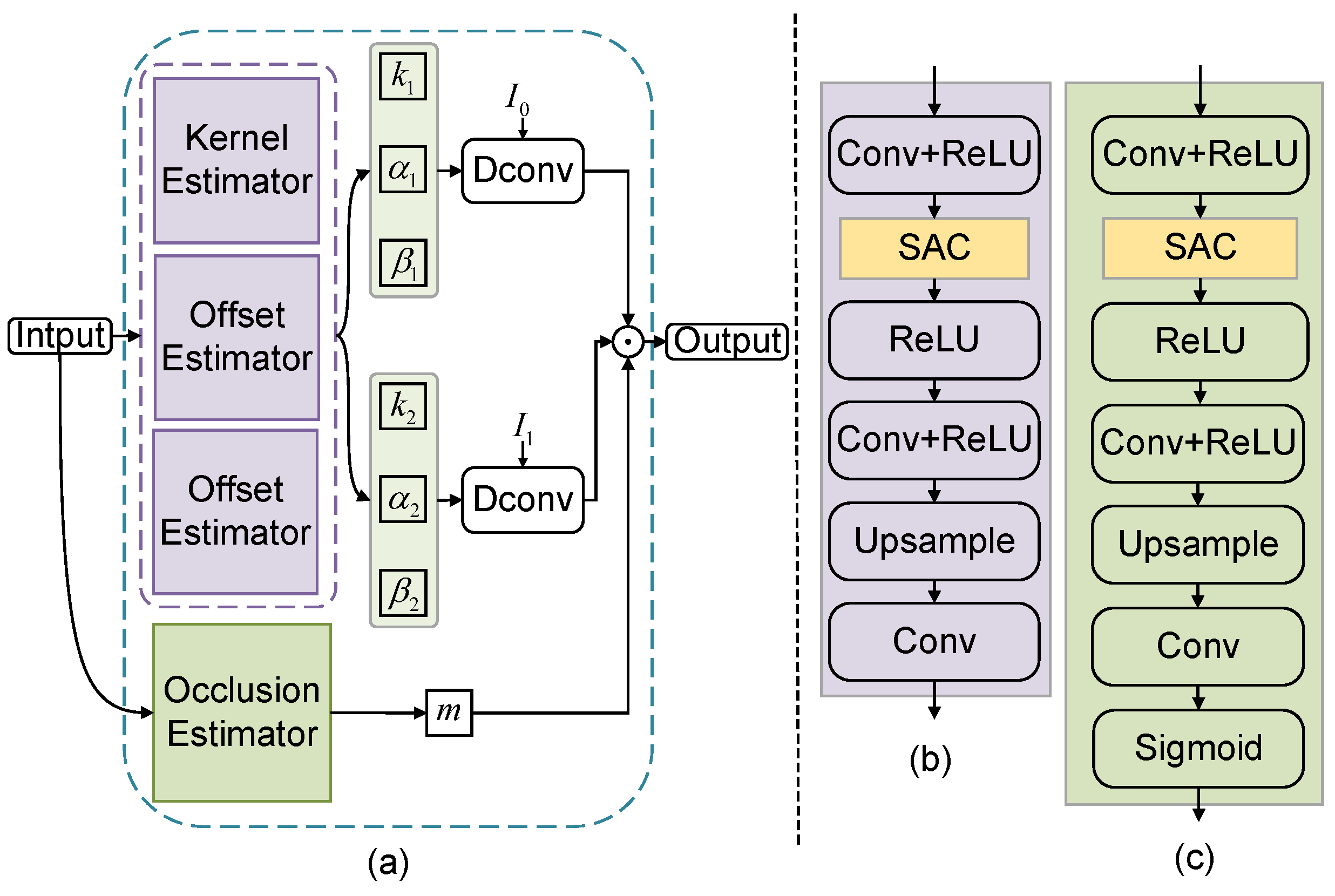
4.4. Deformable Convolutional Synthesis Module

The DConv SynModule is a module used for generating warped frames. As shown in Figure 5, it consists of a kernel estimator, two offset estimators, an occlusion estimator, and deformable convolutions. The four estimators, respectively, estimate the kernel weight k, the offsets $\alpha$ and $\beta$, and the occlusion map m. The deformable convolutions warp them with input frames $I^0$ and $I^1$ to generate $I_t^1$ and $I_t^2$, respectively. Additionally, we enhance the feature space representation by replacing one convolution layer with an SAC module in each estimator.

5. Experiment

5.1. Datasets and Evaluation Metrics

Our model is trained on the ${\mathrm{UHD}}_{\mathrm{Train}}$ dataset and Vimeo90K training set, and evaluated on various datasets.

5.1.1. Training Datasets

• 4K Training Datasets: A training sample is defined as a triplet consisting of two input frames $I_0$ and $I_1$, and the middle frame $I_t$. To investigate the impact of different frame rates on model training, we construct two sets of 4K training datasets from the ${\mathrm{UHD}}_{\mathrm{Train}}$ dataset, based on different temporal distances (TDs). These are set as TD = 1 and TD = 2, respectively, and are denoted as ${\mathrm{UHD}}_{\mathrm{Train}}^{\mathrm{TD}=1}$ and ${\mathrm{UHD}}_{\mathrm{Train}}^{\mathrm{TD}=2}$. Each training dataset comprises 51,840 triplets, with each sample measuring 128 × 128 in size. They are augmented with random flipping and time reversal.
• Benchmark Training Datasets: To more fairly validate the performance of our model, we also train it on Vimeo90K [9]. Its training set contains 51,312 triplets with a resolution of 448 × 256 for training. During training, we randomly crop 192 × 192 patches from the training samples and augment them through random horizontal and vertical flipping and time reversal.

5.1.2. Testing Datasets

• 4K Testing Datasets:${\mathrm{UHD}}_{\mathrm{Text}}$ serves as the 4K testing dataset. To correspond with the training set, ${\mathrm{UHD}}_{\mathrm{Text}}$ is also divided into two testing datasets based on temporal distances (TD = 1 and TD = 2), denoted as ${\mathrm{UHD}}_{\mathrm{Text}}^{\mathrm{TD}=1}$ and ${\mathrm{UHD}}_{\mathrm{Text}}^{\mathrm{TD}=2}$, respectively. Each testing set contains 12 triplets. Due to hardware limitations, we resize the ${\mathrm{UHD}}_{\mathrm{Text}}^{\mathrm{TD}=1}$ and ${\mathrm{UHD}}_{\mathrm{Text}}^{\mathrm{TD}=2}$ to one fourth (1920 × 1080) and one ninth (1280 × 720) of their original size, respectively, denoted as ${\mathrm{UHD}}_{\mathrm{Text}}^{\mathrm{TD}=1}$ (1/4), ${\mathrm{UHD}}_{\mathrm{Text}}^{\mathrm{TD}=1}$ (1/9), ${\mathrm{UHD}}_{\mathrm{Text}}^{\mathrm{TD}=2}$ (1/4), and ${\mathrm{UHD}}_{\mathrm{Text}}^{\mathrm{TD}=2}$ (1/9). When TD = 1, the frame rate increases from 120 fps to 240 fps, and when TD = 2, it increases from 60 fps to 120 fps.
• Vimeo90K: Vimeo90K [9] has been extensively evaluated in recent VFI methods. It contains 3782 triplets with a resolution of 448 × 256.
• UCF101: UCF101 [20] is a collection of videos featuring various human actions, consisting of 379 triplets with a resolution of 256 × 256.
• Middlebury: The resolution of samples in the Middlebury [21] dataset is approximately 640 × 480 pixels. It consists of two subsets, with the OTHER subset providing the ground-truth intermediate frames.

5.1.3. Evaluation Metrics

We use common evaluation metrics in video tasks, including the peak signal-to-noise ratio (PSNR), structural similarity (SSIM) [26], and learned perceptual image patch similarity (LPIPS) [27]. Among these, the higher the better for PSNR and SSIM, and the lower the better for LPIPS.

5.2. Implementation Details

• Network Achitecture: The MPNet comprises four levels of AFE, with a scale factor of 2 at each level and feature channels of 24, 48, 96, and 192. Each AFE contains four SACs, with each SAC possessing five attention heads and a 3 × 3 convolution kernel with stride of 1. The hyperparameter $\lambda$ in SAC that controls the output strength of the convolution is set to 0.3.
• Training Details: Our model is trained end-to-end for 100 epochs by using the Adam optimiser [28], where the hyperparameters ${\beta }_1$, ${\beta }_2$, and ${\beta }_3$ of the optimiser are set to 0.98, 0.92, and 0.99, respectively. The batch size is 8. The initial learning rate is set to ${10}^{-4}$, reduced by a factor of 4 at the 50th, 75th, and 90th epochs. Training takes about four days with two NVIDIA TITAN XP GPUs (manufactured by NVIDIA Corporation, Santa Clara, CA, USA) with PyTorch 1.12.0.

5.3. Comparison to the Previous Methods

5.3.1. Quantitative Comparison

We compare the proposed method with other SOTA VFI methods, including AdaCoF [7], Compressed AdaCoF [8], CDFI [8], RIFE [12], XVFI [5], and FILM [29]. These models are trained using the same strategy on the ${\mathrm{UHD}}_{\mathrm{Train}}$ and evaluated on the ${\mathrm{UHD}}_{\mathrm{Text}}$ with different sizes and temporal distances, as well as on two benchmark datasets, UCF101 [20] and Middlebury [21]. The quantitative experimental results in

Table 1. Quantitative comparisons (PSNR/SSIM/LPIPS) with SOTA methods on different testing datasets, by training with ${\mathrm{UHD}}_{\mathrm{Train}}^{\mathrm{TD}=1}$ and ${\mathrm{UHD}}_{\mathrm{Train}}^{\mathrm{TD}=2}$, respectively. The best and second-best results are colored in red and blue.

Methods	Training Dataset	${\mathbf{UHD}}_{\mathbf{Text}}^{\mathbf{TD}=1}$		${\mathbf{UHD}}_{\mathbf{Text}}^{\mathbf{TD}=2}$		UCF101	Middlebury
		$\mathbf{1}\mathbf{/}\mathbf{4}$	$\mathbf{1}\mathbf{/}\mathbf{9}$	$\mathbf{1}\mathbf{/}\mathbf{4}$	$\mathbf{1}\mathbf{/}\mathbf{9}$
AdaCoF [7]	${\mathrm{UHD}}_{\mathrm{Train}}^{\mathrm{TD}=1}$	40.73/0.954/0.017	39.70/0.940/0.023	34.81/0.909/0.042	33.36/0.887/0.051	34.52/0.944/0.018	33.36/0.936/0.020
Com_AdaCoF [8]		34.04/0.899/0.037	33.88/0.884/0.044	30.18/0.830/0.050	29.83/0.814/0.059	33.30/0.935/0.021	30.93/0.889/0.031
CDFI [8]		39.67/0.946/0.022	38.21/0.925/0.030	32.20/0.872/0.050	31.67/0.857/0.061	34.28/0.942/0.020	32.19/0.911/0.033
RIFE-Large [12]		42.13/0.963/0.019	40.36/0.956/0.022	36.16/0.947/0.032	35.69/0.907/0.045	34.81/0.949/0.018	34.29/0.949/0.018
XVFI [5]		42.35/0.964/0.018	41.10/0.959/0.021	36.19/0.953/0.031	35.73/0.908/0.040	34.95/0.950/0.016	34.36/0.949/0.017
FILM-${\mathcal{L}}_{\mathcal{S}}$ [29]		42.37/0.967/-	42.74/0.966/-	36.82/0.934/-	37.85/0.928/-	34.40/0.946/-	34.66/0.950/-
Ours		42.47/0.965/0.017	41.31/0.959/0.020	36.30/0.955/0.031	35.87/0.909/0.043	34.75/0.947/0.017	34.63/0.950/0.017
AdaCoF [7]	${\mathrm{UHD}}_{\mathrm{Train}}^{\mathrm{TD}=2}$	40.05/0.949/0.018	38.66/0.934/0.026	35.78/0.917/0.034	35.00/0.897/0.044	34.08/0.938/0.020	31.40/0.897/0.029
Com_AdaCoF [8]		39.24/0.945/0.020	38.50/0.931/0.026	35.70/0.914/0.034	34.71/0.891/0.043	33.10/0.932/0.023	30.46/0.875/0.034
CDFI [8]		40.58/0.955/0.020	39.37/0.942/0.027	35.54/0.922/0.036	35.15/0.902/0.047	33.87/0.943/0.019	32.31/0.923/0.029
RIFE-Large [12]		41.57/0.959/0.019	40.51/0.953/0.024	37.69/0.949/0.032	36.63/0.914/0.044	34.85/0.950/0.019	33.88/0.941/0.025
XVFI [5]		41.69/0.961/0.018	40.60/0.954/0.023	37.73/0.951/0.031	36.74/0.916/0.042	34.99/0.951/0.017	33.90/0.942/0.023
FILM-${\mathcal{L}}_{\mathcal{S}}$ [29]		42.19/0.967/-	41.67/0.964/-	38.27/0.940/-	37.76/0.932/-	34.12/0.944/-	34.26/0.945/-
Ours		41.80/0.962/0.019	40.82/0.956/0.022	37.80/0.952/0.030	36.92/0.917/0.042	34.83/0.948/0.017	34.04/0.943/0.021

demonstrate that our model achieves the best performance on ${\mathrm{UHD}}_{\mathrm{Text}}^{\mathrm{TD}=1}$$(1/4)$ and also shows excellent performance on other testing datasets. Specifically, when trained on ${\mathrm{UHD}}_{\mathrm{Train}}^{\mathrm{TD}=1}$, our model outperforms XVFI [5] by 0.12 dB and FILM [29] by 0.10 dB on ${\mathrm{UHD}}_{\mathrm{Text}}^{\mathrm{TD}=1}$ (1/4). These results provide evidence of the superior performance of our model in handling 4K videos. Furthermore, the results in the table confirm the impact of different frame rates and resolutions of the datasets on the performance of VFI models. This method of cross-validation by different training and test sets side-by-side reflects the importance of the dataset for VFI tasks with different scenarios. In addition, we find that our model outperforms FILM [29] by 0.35 dB and 0.71 dB on UCF101 [20], when trained on ${\mathrm{UHD}}_{\mathrm{Train}}$ with TD = 1 and TD = 2, respectively.

To further evaluate the generalisation performance of our model, we train it on the Vimeo90K [9] dataset and compare it with 13 SOTA VFI methods on three benchmark datasets. Due to hardware limitations and to expedite the exploration process, we directly use the reported results of SepCov [16], CtxSyn [30], SoftSplat [31], DAIN [14], RIFE [12], and IFRNet [15] as baselines, which were previously reported in [15,31]. As shown in

Table 2. Quantitative comparison of our method with 13 SOTA methods on the Vimeo90K [9] dataset. #Params represents the number of parameters of the networks. ^† denotes the results from Ref. [31]. ^‡ denotes the results from Ref. [15]. The best and second-best results are colored in red and blue.

Methods	Training Dataset	#Params	Vimeo90K	UCF101	Middlebury
† $\mathrm{SepConv}—{\mathcal{L}}_1$ [16]	proprietary	21.6 M	33.80/0.956/0.027	34.79/0.947/0.029	35.73/0.959/0.017
† $\mathrm{SepConv}—{\mathcal{L}}_F$ [16]	proprietary	21.6 M	33.45/0.951/0.019	34.69/0.945/0.024	35.03/0.954/0.013
† $\mathrm{CtxSyn}—{\mathcal{L}}_{Lap}$ [1]	proprietary	-	34.39/0.961/0.024	34.62/0.949/0.031	36.93/0.964/0.016
† $\mathrm{CtxSyn}—{\mathcal{L}}_F$ [1]	proprietary	-	33.76/0.955/0.017	34.01/0.941/0.024	35.95/0.959/0.013
† $\mathrm{SoftSplat}—{\mathcal{L}}_{Lap}$ [31]	Vimeo90K (256 × 256)	-	36.10/0.970/0.021	35.39/0.952/0.033	38.42/0.971/0.016
† $\mathrm{SoftSplat}—{\mathcal{L}}_F$ [31]	Vimeo90K (256 × 256)	-	35.48/0.964/0.013	35.10/0.948/0.022	37.55/0.965/0.008
† $\mathrm{DAIN}$ [14]	Vimeo90K (256 × 256)	24.02 M	34.70/0.964/0.022	35.00/0.950/0.028	36.70/0.965/0.017
BMBC [32]	Vimeo90K (448 × 256)	11.0 M	35.06/0.964/0.015	35.16/0.950/0.019	36.79/0.965/0.015
CAIN [33]	Vimeo90K (448 × 256)	42.8 M	34.65/0.959/0.020	34.98/0.950/0.021	35.11/0.951/0.019
CDFI [8]	Vimeo90K (448 × 256)	4.98 M	35.17/0.964/0.010	35.21/0.950/0.015	37.14/0.966/0.007
AdaCoF [7]	Vimeo90K (448 × 256)	22.93 M	34.56/0.959/0.018	35.16/0.950/0.019	36.09/0.962/0.017
EDSC-${\mathcal{L}}_{\mathcal{C}}$ [19]	Vimeo90K (448 × 256)	8.9 M	34.86/0.962/0.016	35.17/0.950/0.019	36.76/0.966/0.014
EDSC-${\mathcal{L}}_{\mathcal{F}}$ [19]	Vimeo90K (448 × 256)	8.9 M	34.57/0.958/0.010	35.04/0.948/0.015	36.48/0.963/0.007
‡ $\mathrm{RIFE}-\mathrm{Large}$ [12]	Vimeo90K (224 × 224)	9.8 M	35.62/0.978/ -	35.28/0.969/ -	-
‡ $\mathrm{IFRNet}-\mathrm{Large}$ [15]	Vimeo90K (224 × 224)	19.7 M	36.20/0.980/ -	35.42/0.969/ -	-
FILM-${\mathcal{L}}_{\mathcal{S}}$ [29]	Vimeo90K (256 × 256)	-	35.87/0.968/ -	35.16/0.949/ -	37.57/0.966/ -
XVFI [5]	Vimeo90K (256 × 256)	5.5 M	35.07/0.968/ -	35.18/0.951/ -	-
Ours	Vimeo90K (192 × 192)	5.8 M	36.23/0.971/0.008	34.29/0.945/0.016	35.30/0.958/0.009

, our model outperforms IFRNet-Large [15] and XVFI [5] by 0.03 dB and 1.16 dB on the Vimeo90K [9] testing set, respectively. Compared to FILM [29], our model outperforms it by 0.36 dB. These results indicate that our model is also suitable for low-resolution VFI tasks.

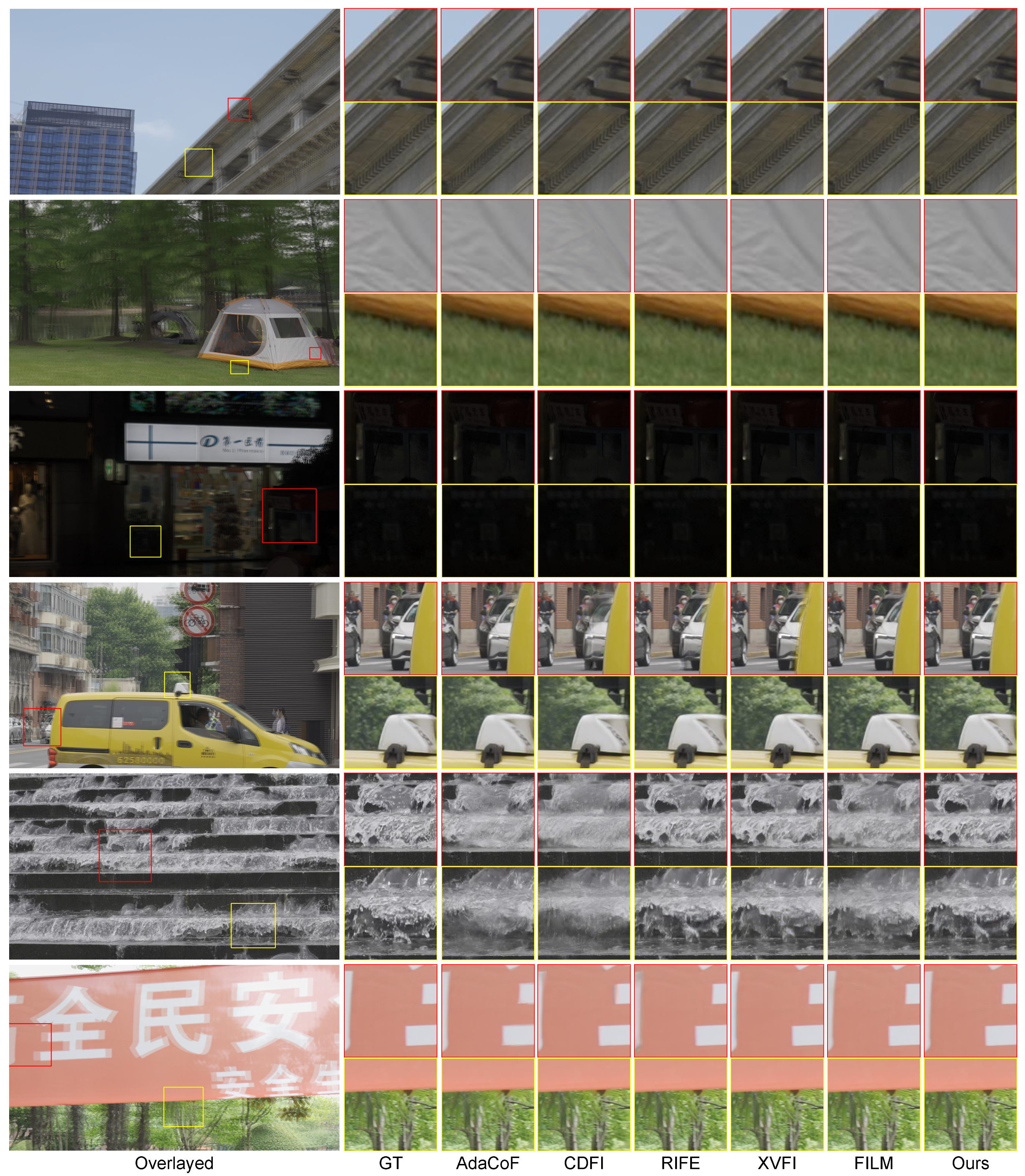
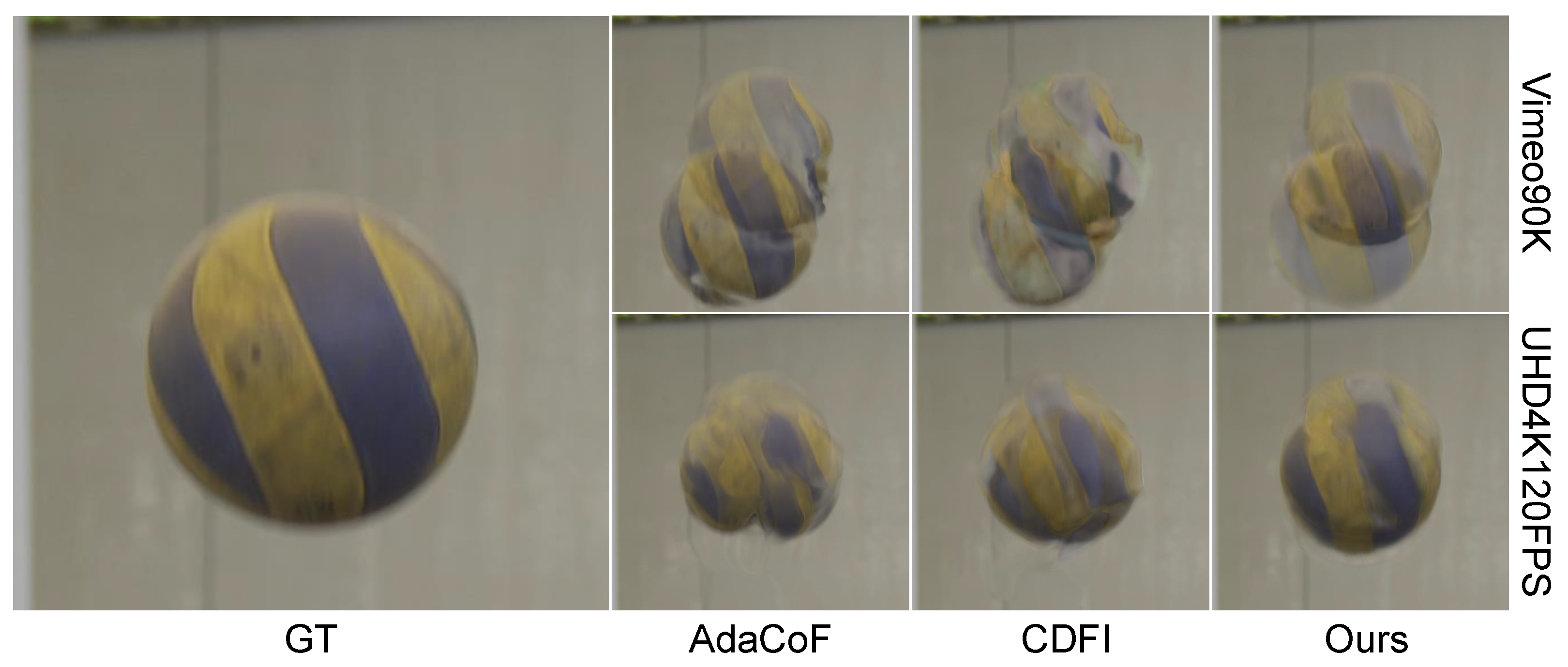
5.3.2. Qualitative Comparison

Figure 6 shows the visual results of our method compared to other SOTA methods on ${\mathrm{UHD}}_{\mathrm{Text}}$. In the 4th and 5th examples, our method successfully interpolates the intermediate frames of fast-moving wheels and flowing water. In the remaining examples, our method also produces more realistic interpolation results. In particular, note that in comparison with the quantisation results in Table 1, although some of the quantisation results of our model are slightly lower than the those of the SOTA methods, our method generates more realistic 4K video frames, which also illustrates the superiority of our method in processing 4K videos.

5.4. Ablation Study

This section describes the ablation study performed on our method to validate the effectiveness of MPNet, CEModule, and SAC.

5.4.1. Quantitative Comparison

• Effect of the SAC: SAC determines the range of pixel information captured by the model and its computational cost, so we conduct an ablation study on SAC to examine its impact. The experimental results are shown in

  Table 3. Ablation study of SAC.

  Number of SAC	Training Dataset	$1/4$
  		${\mathrm{UHD}}_{\mathrm{Text}}^{\mathrm{TD}=1}$	${\mathrm{UHD}}_{\mathrm{Text}}^{\mathrm{TD}=2}$
  0	${\mathrm{UHD}}_{\mathrm{Train}}^{\mathrm{TD}=2}$	37.86/0.930/0.028	34.44/0.898/0.048
  1		35.94/0.917/0.029	31.55/0.847/0.053
  2		41.47/0.964/0.017	37.63/0.931/0.033
  4		41.80/0.962/0.019	37.80/0.952/0.030
  6		41.75/0.963/0.018	38.02/0.934/0.033

  , demonstrating that the model performs poorly when it lacks SAC. On ${\mathrm{UHD}}_{\mathrm{Text}}^{\mathrm{TD}=1}$, the model achieves the highest PSNR of 41.80 dB when the number of SAC is 4, and the overall performance is optimal when the number of SAC is 6. To balance model performance and computational cost, we set SAC to 4 in the experiments. Notably, the model with one SAC performs 1.92 dB less than the model without SAC. This result suggests that when only one SAC is used, it leads to worse model performance. It can also be shown that the fixed-size convolution kernel weakens its ability to learn long-range information correlation when the information captured by a single attention is passed to the convolutional layers.

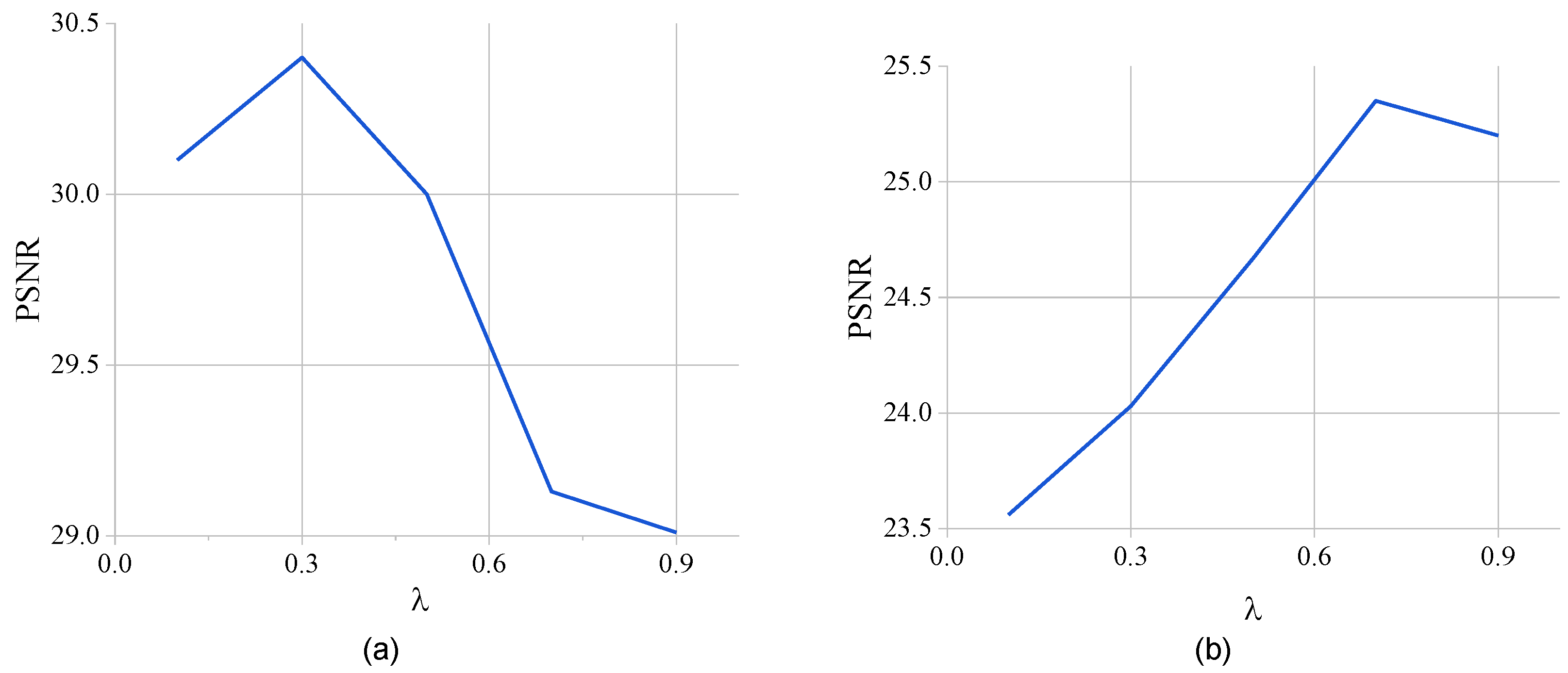
• Effect of the hyperparameter $\lambda$: To investigate the sensitivity of the hyperparameter $\lambda$ to the strength of the convolutional output in SAC, we design two models with different numbers of layers, as shown in Figure 7. Figure 7 presents the complete model, and Figure 7b presents the model in the encoder of MPNet that contains only two AFE layers. Both models were trained and tested under the Vimeo90K [9] dataset with 30 epochs in total. The comparison shows that when there are fewer network layers, $\lambda$ is larger and it is easier for convolution to extract features than attention. On the contrary, in more network layers, when the convolution output strength $\lambda$ is larger, it will affect the ability of attention to extract features. And the larger the $\lambda$, the more pronounced this effect is. Finally, in order to balance the model performance, we set $\lambda$ = 0.3. This result also motivates us to explore learnable hyperparameters in the future.

• Effect of the MPNet. MPNet and AFE are used to capture the long-range dependency of pixels and perform multi-scale feature extraction and fusion. To evaluate their impact on model performance, we replace MPNet with U-Net and AFE with multilayer convolution, both containing the same number of SACs. The experimental results in

  Table 4. Ablation study on the proposed modules. Training dataset is ${\mathrm{UHD}}_{\mathrm{Train}}^{\mathrm{TD}=2}$. ✓ means with, ✗ means without.

  	Backbone	SAC	CEModule	Number	${\mathbf{UHD}}_{\mathbf{Text}}^{\mathbf{TD}=2}$		UCF101	Middlebury
  				of AEF	1/4	1/9
  Model 1	MPNet	✓	✗	4	37.35/0.925/0.033	36.29/0.905/0.043	34.37/0.942/0.019	32.81/0.928/0.023
  Model 2	MPNet	✓	✓	3	37.53/0.929/0.035	36.53/0.912/0.044	34.40/0.945/0.018	33.06/0.929/0.026
  Model 3	U-Net	✓	✓	–	37.74/0.930/0.034	36.62/0.909/0.043	34.53/0.945/0.018	32.88/0.918/0.025
  Model 4	MPNet	✓	✓	4	37.80/0.952/0.030	36.92/0.917/0.042	34.83/0.948/0.017	34.04/0.943/0.021

  demonstrate that Model 4 (complete model) exhibits the best performance on our dataset and two benchmark datasets. Specifically, on ${\mathrm{UHD}}_{\mathrm{Text}}^{\mathrm{TD}=2}$ (1/4) and ${\mathrm{UHD}}_{\mathrm{Text}}^{\mathrm{TD}=2}$ (1/9), Model 4 achieves PSNR over Model 3 (based on U-Net) by 0.06 dB and 0.3 dB, respectively. This highlights the importance of multi-scale information extraction and fusion for high-resolution videos. Additionally, comparing Model 4 with Model 2 reveals that the number of AFE layers significantly affects the ability of the model to learn multi-scale features.

• Effect of the CEModule. In Table 4, by comparing the results of Model 1 (without CEModule) and Model 4, we observe that the PSNR of ${\mathrm{UHD}}_{mathrmText}^{\mathrm{TD}=2}$ (1/4) and ${\mathrm{UHD}}_{mathrmText}^{\mathrm{TD}=2}$ (1/9) improves by 0.45 dB and 0.63 dB, respectively, while the LPIPS is reduced by 0.003 and 0.001, respectively. These findings indicate that the inclusion of CEModule significantly enhances the performance of the model. CEModule helps SAC learn contextual information and enhances the ability of the model to capture global information. Furthermore, these results further validate the effectiveness and adaptability of our model in high-resolution VFI tasks. Also, comparing the LPIPS of Model 4 and Model 1, although the change in their values is not obvious, in Figure 8, we can see a significant difference in the visualisation results (detail in Section 5.4.2).

5.4.2. Qualitative Comparison

The visualisation results of the ablation study are shown in Figure 8. We find that models without CEModule or SAC cause severe motion blur when handling rotating objects. Comparing the results in the last row of the figure, it is evident that models without CEModule or MPNet perform poorly in handling edge cases where multiple objects intersect, demonstrating the effectiveness of our model in extracting and fusing multi-scale information in complex scenes. Overall, our model consistently produces clearer results and finer details when dealing with multi-object scenes, rotations, and large motions, showcasing its robustness in challenging scenarios.

In addition, we perform a multi-frame interpolation visualisation study to check the performance of the model, by recursively applying our model to generate intermediate frames. The interpolation results on the ${\mathrm{UHD}}_{\mathrm{Text}}$ are shown in Figure 9, where both examples contain large motion with a temporal distance of 4 between input frames, equivalent to 30 fps. We perform 8× interpolations, which corresponds to increasing the frame rate to 240 fps. The results show that our model generates multiple intermediate frames with smooth motion, which can indicate the applicability of our model for multi-frame interpolation tasks.

6. Conclusions

In this paper, we first propose a novel high-quality UHD dataset called UHD4K120FPS containing large motion and complex textures. Then, we propose a new model for 4K VFI tasks. We design attention based on simple mapping and convolutional enhancement to capture the long-distance dependence of pixels in 4K video, while our model can efficiently learn and fuse multi-scale information, which enables our model to handle large motion and complex scenes in 4K videos. Moreover, our method achieves SOTA performance on UHD4K120FPS and several low-resolution benchmark datasets.

Similar to existing frame interpolation methods [7,8,29], we only synthesise the middle frames. In future work, we will explore time variables to extend to arbitrary-time-frame interpolation and multi-frame interpolation, while also optimising the computational efficiency of the model for real-time applications.

References

1. Niklaus, S.; Liu, F. Context-aware synthesis for video frame interpolation. In Proceedings of the IEEE Conference on Computer Vision and Pattern Recognition, Salt Lake City, UT, USA, 18–23 June 2018; pp. 1701–1710. [Google Scholar]
2. Haris, M.; Shakhnarovich, G.; Ukita, N. Space-time-aware multi-resolution video enhancement. In Proceedings of the IEEE/CVF Conference on Computer Vision and Pattern Recognition, Seattle, WA, USA, 13–19 June 2020; pp. 2859–2868. [Google Scholar]
3. Wu, C.Y.; Singhal, N.; Krahenbuhl, P. Video compression through image interpolation. In Proceedings of the European Conference on Computer Vision (ECCV), Munich, Germany, 8–14 September 2018; pp. 416–431. [Google Scholar]
4. Kalantari, N.K.; Wang, T.C.; Ramamoorthi, R. Learning-based view synthesis for light field cameras. ACM Trans. Graph. TOG 2016, 35, 193. [Google Scholar] [CrossRef]
5. Sim, H.; Oh, J.; Kim, M. Xvfi: Extreme video frame interpolation. In Proceedings of the IEEE/CVF International Conference on Computer Vision, Montreal, QC, Canada, 10–17 October 2021; pp. 14489–14498. [Google Scholar]
6. Ahn, H.E.; Jeong, J.; Kim, J.W. A fast 4k video frame interpolation using a hybrid task-based convolutional neural network. Symmetry 2019, 11, 619. [Google Scholar] [CrossRef]
7. Lee, H.; Kim, T.; Chung, T.Y.; Pak, D.; Ban, Y.; Lee, S. AdaCoF: Adaptive collaboration of flows for video frame interpolation. In Proceedings of the IEEE/CVF Conference on Computer Vision and Pattern Recognition, Seattle, WA, USA, 13–19 June 2020; pp. 5315–5324. [Google Scholar]
8. Ding, T.; Liang, L.; Zhu, Z.; Zharkov, I. Cdfi: Compression-driven network design for frame interpolation. In Proceedings of the IEEE/CVF Conference on Computer Vision and Pattern Recognition, Nashville, TN, USA, 20–25 June 2021; pp. 8001–8011. [Google Scholar]
9. Xue, T.; Chen, B.; Wu, J.; Wei, D.; Freeman, W. Video enhancement with task-oriented flow. Int. J. Comput. Vis. 2018, 127, 1106–1125. [Google Scholar] [CrossRef]
10. Vaswani, A.; Shazeer, N.; Parmar, N.; Uszkoreit, J.; Jones, L.; Gomez, A.N.; Kaiser, Ł.; Polosukhin, I. Attention is all you need. In Proceedings of the 31st International Conference on Neural Information Processing Systems, Long Beach, CA, USA, 4–9 December 2017; pp. 6000–6010. [Google Scholar]
11. Liu, Z.; Yeh, R.A.; Tang, X.; Liu, Y.; Agarwala, A. Video frame synthesis using deep voxel flow. In Proceedings of the IEEE International Conference on Computer Vision, Venice, Italy, 22–29 October 2017; pp. 4463–4471. [Google Scholar]
12. Huang, Z.; Zhang, T.; Heng, W.; Shi, B.; Zhou, S. Real-time intermediate flow estimation for video frame interpolation. In Proceedings of the European Conference on Computer Vision (ECCV), Tel Aviv, Israel, 23–27 October 2022; pp. 624–642. [Google Scholar]
13. Jiang, H.; Sun, D.; Jampani, V.; Yang, M.H.; Learned-Miller, E.; Kautz, J. Super slomo: High quality estimation of multiple intermediate frames for video interpolation. In Proceedings of the IEEE Conference on Computer Vision and Pattern Recognition, Salt Lake City, UT, USA, 18–23 June 2018; pp. 9000–9008. [Google Scholar]
14. Bao, W.; Lai, W.S.; Ma, C.; Zhang, X.; Gao, Z.; Yang, M.H. Depth-aware video frame interpolation. In Proceedings of the IEEE/CVF Conference on Computer Vision and Pattern Recognition, Long Beach, CA, USA, 15–20 June 2019; pp. 3703–3712. [Google Scholar]
15. Kong, L.; Jiang, B.; Luo, D.; Chu, W.; Huang, X.; Tai, Y.; Wang, C.; Yang, J. Ifrnet: Intermediate feature refine network for efficient frame interpolation. In Proceedings of the IEEE/CVF Conference on Computer Vision and Pattern Recognition, New Orleans, LA, USA, 18–24 June 2022; pp. 1969–1978. [Google Scholar]
16. Niklaus, S.; Liu, F. Sepconv: Separable convolution for fast video interpolation. In Proceedings of the IEEE International Conference on Computer Vision, Venice, Italy, 22–29 October 2017; pp. 261–270. [Google Scholar]
17. Niklaus, S.; Mai, L.; Liu, F. Video frame interpolation via adaptive convolution. In Proceedings of the IEEE Conference on Computer Vision and Pattern Recognition, Honolulu, HI, USA, 21–26 July 2017; pp. 2270–2279. [Google Scholar]
18. Zhu, X.; Hu, H.; Lin, S.; Dai, J. Deformable convnets v2: More deformable, better results. In Proceedings of the IEEE/CVF Conference on Computer Vision and Pattern Recognition, Long Beach, CA, USA, 15–20 June 2019; pp. 9308–9316. [Google Scholar]
19. Cheng, X.; Chen, Z. Multiple video frame interpolation via enhanced deformable separable convolution. IEEE Trans. Pattern Anal. Mach. Intell. 2021, 44, 7029–7045. [Google Scholar] [CrossRef] [PubMed]
20. Soomro, K.; Zamir, A.R.; Shah, M. UCF101: A dataset of 101 human actions classes from videos in the wild. arXiv 2012, arXiv:1212.0402. [Google Scholar]
21. Baker, S.; Scharstein, D.; Lewis, J.; Roth, S.; Black, M.J.; Szeliski, R. A database and evaluation methodology for optical flow. Int. J. Comput. Vis. 2007, 92, 1–31. [Google Scholar] [CrossRef]
22. Kim, S.Y.; Oh, J.; Kim, M. Fisr: Deep joint frame interpolation and super-resolution with a multi-scale temporal loss. In Proceedings of the AAAI Conference on Artificial Intelligence, New York, NY, USA, 7–12 February 2020; Volume 34, pp. 11278–11286. [Google Scholar]
23. Zhao, S.; Zhao, L.; Zhang, Z.; Zhou, E.; Metaxas, D. Global matching with overlapping attention for optical flow estimation. In Proceedings of the IEEE/CVF Conference on Computer Vision and Pattern Recognition, New Orleans, LA, USA, 18–24 June 2022; pp. 17592–17601. [Google Scholar]
24. Zhao, H.; Shi, J.; Qi, X.; Wang, X.; Jia, J. Pyramid scene parsing network. In Proceedings of the IEEE Conference on Computer Vision and Pattern Recognition, Honolulu, HI, USA, 21–26 July 2017; pp. 2881–2890. [Google Scholar]
25. Pan, X.; Ge, C.; Lu, R.; Song, S.; Chen, G.; Huang, Z.; Huang, G. On the integration of self-attention and convolution. In Proceedings of the IEEE/CVF Conference on Computer Vision and Pattern Recognition, New Orleans, LA, USA, 18–24 June 2022; pp. 815–825. [Google Scholar]
26. Wang, Z.; Bovik, A.C.; Sheikh, H.R.; Simoncelli, E.P. Image quality assessment: From error visibility to structural similarity. IEEE Trans. Image Process. 2004, 13, 600–612. [Google Scholar] [CrossRef]
27. Zhang, R.; Isola, P.; Efros, A.A.; Shechtman, E.; Wang, O. The unreasonable effectiveness of deep features as a perceptual metric. In Proceedings of the IEEE Conference on Computer Vision and Pattern Recognition, Salt Lake City, UT, USA, 18–23 June 2018; pp. 586–595. [Google Scholar]
28. Xie, X.; Zhou, P.; Li, H.; Lin, Z.; Yan, S. Adan: Adaptive Nesterov Momentum Algorithm for Faster Optimizing Deep Models. arXiv 2022, arXiv:2208.06677. [Google Scholar]
29. Reda, F.; Kontkanen, J.; Tabellion, E.; Sun, D.; Pantofaru, C.; Curless, B. Film: Frame interpolation for large motion. In Proceedings of the European Conference on Computer Vision, Tel Aviv, Israel, 23–27 October 2022; Springer: Berlin/Heidelberg, Germany, 2022; pp. 250–266. [Google Scholar]
30. Peleg, T.; Szekely, P.; Sabo, D.; Sendik, O. Im-net for high resolution video frame interpolation. In Proceedings of the IEEE/CVF Conference on Computer Vision and Pattern Recognition, Long Beach, CA, USA, 15–20 June 2019; pp. 2393–2402. [Google Scholar]
31. Niklaus, S.; Liu, F. Softmax splatting for video frame interpolation. In Proceedings of the IEEE/CVF Conference on Computer Vision and Pattern Recognition, Seattle, WA, USA, 13–19 June 2020; pp. 5437–5446. [Google Scholar]
32. Park, J.; Ko, K.; Lee, C.; Kim, C.S. Bmbc: Bilateral motion estimation with bilateral cost volume for video interpolation. In Proceedings of the European Conference on Computer Vision, Glasgow, UK, 23–28 August 2020; pp. 109–125. [Google Scholar]
33. Choi, M.; Kim, H.; Han, B.; Xu, N.; Lee, K.M. Channel attention is all you need for video frame interpolation. In Proceedings of the AAAI Conference on Artificial Intelligence, New York, NY, USA, 7–12 February 2020; Volume 34, pp. 10663–10671. [Google Scholar]
Figure 1. Visual comparison of our method with 2 state-of-the-art (SOTA) methods on UHD4K120FPS testing dataset. The 2 SOTA methods are AdaCoF [7] and CDFI [8]. The training datasets are Vimeo90K [9] dataset with a resolution of 448 × 256 and UHD4K120FPS with a resolution of 3840 × 2160. GT: Ground Truth.
Electronics 13 01037 g001
Figure 2. Some examples of the UHD4K120FPS dataset and their oscilloscope display. In each example figure, above is the original image, below left is the brightness waveform graph displayed by the oscilloscope, and below right is the colour space histogram. The numbers indicate the magnitude of the optical flow between input frames in 30 fps.
Electronics 13 01037 g002
Figure 3. Overview of our proposed framework.
Electronics 13 01037 g003
Figure 4. The structural diagrams of MPNet, AEF, and SAC: (a) MPNet; (b) AFE; (c) SAC.
Electronics 13 01037 g004
Figure 5. The structural diagrams of DConv SynModule: (a) DConv SynModule; (b) kernel estimator and offset estimators; (c) occlusion estimator.
Electronics 13 01037 g005
Figure 6. Visual comparisons of different VFI methods on UHD Text TD = 2 ( 1 / 4 ) . Training dataset is UHD Train TD = 2 .
Electronics 13 01037 g006
Figure 7. Sensitivity of the hyperparameter λ to the strength of the convolutional output in network models with different numbers of AEF layers. (a) The complete model. (b) The model with 2 AFE layers in the encoder of the MPNet.
Electronics 13 01037 g007
Figure 8. Visual comparisons of ablation study on UHD Text TD = 2 (1/4). Training dataset is UHD Train TD = 2 . w/o means without, CE is CEModule, and MP is MPNet.
Electronics 13 01037 g008
Figure 9. Visualisation results of our method for multi-frame interpolation on the UHD Text . Time variables { t = 0.125 , t = 0.25 , , t = 0.875 } denote temporal points between 0 and 1.
Electronics 13 01037 g009