Review of Matrix Rank Constraint Model for Impulse Interference Image Inpainting

Abstract

Camera failure or loss of storage components in imaging equipment may result in the loss of important image information or random pulse noise interference. The low-rank prior is one of the most important priors in image optimization processing. This paper reviews and compares some low-rank constraint models for image matrices. Firstly, an overview of image-inpainting models based on nuclear norm, truncated nuclear norm, weighted nuclear norm, and matrix-factorization-based F norm is presented, and corresponding optimization iterative algorithms are provided. Then, we use different image matrix low-order constraint models to recover satellite images from three types of pulse interference and provide our experimental visual and numerical results. Finally, it can be concluded that the method based on the weighted nuclear norm can achieve the best image restoration effect. The F norm method based on matrix factorization has the shortest computational time and can be used for large-scale low-rank matrix calculations. Compared with nuclear norm-based methods, weighted nuclear norm-based methods and truncated nuclear norm-based methods can significantly improve repair performance.

1. Introduction

In machine vision applications, images often suffer from impulse interference due to various factors such as pulse noise caused by detector pixel failure in the camera or loss of storage elements in the imaging equipment [1]. Satellite images, unmanned aerial vehicle (UAV) images, etc. generally have local smoothness, so their two-dimensional representation matrices usually have obvious low rankness. Low-rank prior information has excellent performance in image denoising [1], inpainting [2,3], reconstruction [4], deblurring [5], and other signal optimization processing fields. In existing low-matrix-rank-based image-inpainting methods, low-rank prior information is mainly divided into the low rank of the signal itself, such as the inherent low rank of the matrix, and the similarity of local map block information [6], the similarity between frames of a video [7], etc. A low-rank matrix with a Hankel-like structure can be constructed in the Fourier domain by using the annihilating filter relationship [2,4]. A high-order tensor rank can be obtained under various tensor decomposition frameworks, such as CANECOMP/PARAFAC (CP), Tucker [8,9], tensor train (TT) [10], and tensor singular value decomposition (t-SVD) [11].

In addition to the low-rank prior, early image-denoising methods assumed that images had sparse representations in their transformation domains, such as the difference domain, wavelet domain, etc. [12,13]. Following this assumption, the sparse prior information was then constrained to recover the image from the noise. Due to the effectiveness of low rank and sparsity in constrained image optimization problems, image-processing schemes that combine constrained sparsity with low-rank prior information have been continuously proposed [14,15]. Some image-denoising methods use decomposition models of low rank and sparse components, such as the robust principal component analysis (RPCA) method [16], aimed at separating low-rank images from sparse interference images. With the progress in the research and development of tensor decomposition tools in the field of mathematics, such as t-SVD, TT decomposition, etc. [10,11,17], related image or video optimization applications based on a low-rank tensor are also being developed [18,19,20,21,22].

In addition to using low-rank prior information to construct the constraint model for impulse interference image inpainting, many theories, methods, and technologies in the field of signal processing can be combined to solve image-inpainting problems, such as various matrix/tensor completion theories in mathematics [18,23,24], finite innovation rate (FIR) theory [25], image and video enhancing (such as Hankel-like-matrix-based technology [1,2,4]), denoising schemes (such as the famous BM3D image-denoising technology [26] and nonlocal TV denoising technology [12]), etc. Various tensor-decomposition-based completion methods, convex optimization schemes, and fast optimization algorithm research systems can also be used to optimize image-inpainting methods.

The above methods are inseparable from the most basic problems in modeling and solving matrix low-rank constraints. The initial modeling method is to establish a constraint minimizing the number of nonzero singular values in the matrix, i.e., minimizing the $l_0$ norm, but this is an NP-hard problem that cannot be solved. In order to approximate the optimal solution, various matrix low-rank constraint modeling schemes have been proposed to replace the $l_0$ norm, such as the $l_{\mathrm{p}}$ norm, weighted nuclear norm, truncated nuclear norm, matrix factorization replacing nuclear norm, and so on. However, to our knowledge, there has been no literature review or comparison of these methods in dealing with the same optimization problem.

This paper uses the low-rank property of the image matrix to optimize the image-inpainting model and algorithm under three kinds of pulse interference. Image-inpainting-modeling schemes based on the nuclear norm, truncated nuclear norm, weighted nuclear norm, and matrix-factorization-based F norm are reviewed, and their corresponding optimization iterative algorithms, such as the TSVT_ADMM algorithm, WSVT_ADMM algorithm, and UV_ADMM algorithm, are given. The experimental results of various inpainting methods are displayed visually and numerically, and a comparative analysis is given.

The structure and content of this paper are arranged as follows: Section 1 presents an introduction; Section 2 establishes the basis of the matrix low-rank constraint inpainting model and solution algorithm; Section 3 presents the experimental comparison; and the last section presents the conclusions.

2. The Matrix Low-Rank Constrained Inpainting Model and Its Solution Algorithm

Image-inpainting models based on a low-rank matrix are generally expressed as follows:

$$\stackrel{\wedge }{X}=\arg \underset{X}{\min } rank(\Phi X) s.t. Y-{\Theta }_{\Omega }X\le \epsilon$$

(1)

where $X$ represents the image ($X\in R^2$ grayscale value image, $X\in R^3$ RGB image, grayscale value video, etc.); ${\Theta }_{\Omega }$ represents the interference operator, in which the set of interference pixel positions is $\Omega$; $\stackrel{\wedge }{X}$ represents the optimal solution; $Y$ represents the interfered image; $\epsilon$ represents the error, generally set as a small constant value matrix, such as constant 10⁻¹⁴; $\Phi$ represents the low-rank transformation operation; and $\Phi X$ is used to transform $X$ into a matrix or tensor with low ranks, such as a low-rank matrix transformed by similar blocks of local images, a low-rank structure matrix [1,2,4] transformed by the relationship of the annihilating filter, or a low-rank matrix [7] transformed by the similarity between frames. If videos or RGB images are treated as third-order or higher-order tensors, the rank property may come from the tensor Tucker rank [27], TT rank [19], etc. Under the interference of impulse noise, the ${\Theta }_{\Omega }$ operator generally has three representations, as detailed below.

The first representation is random-valued impulse noise (RVIN) [1]:

$${\Theta }_{\Omega }X(i, j)=\left\{\begin{array}{ll}V(i, j) , (i, j)\in \Omega & \mathrm{with} \mathrm{random} \mathrm{probability}p\\ X(i, j) , (i, j)\notin \Omega & \mathrm{with} \mathrm{random} \mathrm{probability} 1-p\end{array}\right.$$

The value of $V$ is random, and its range is within the range of $X$’s pixel value, such as the range of 0~255, or the range of normalized 0~1. $p$ is the interference rate, that is, the percentage of the number of interfering pixels in the total number of pixels in the image.

The second representation is salt and pepper noise, a special kind of RVIN [1]:

$${\Theta }_{\Omega }X(i, j)=\left\{\begin{array}{ll}{V}_{\max } , (i, j)\in \Omega & \mathrm{with} \mathrm{random} \mathrm{probability}\frac{p}{2}\\ V_{\min } , (i, j)\in \Omega & \mathrm{with} \mathrm{random} \mathrm{probability}\frac{p}{2}\\ X(i, j), (i, j)\notin \Omega & \mathrm{with} \mathrm{random} \mathrm{probability} 1-p\end{array}\right.$$

where $V_{\max }$ is the maximum value of salt and pepper noise and $V_{\min }$ is the minimum value of salt and pepper noise.

In addition, random pixel loss is also a typical problem in the research field of image repair [2,6,8]:

$${\Theta }_{\Omega }X(i, j)=\left\{\begin{array}{cc}\hfill 0\hspace{1em},\hspace{1em} (i, j)\in \Omega \hfill & \mathrm{Random} \mathrm{probability} p\hfill \\ \hfill X(i, j) , (i, j)\notin \Omega \hfill & \mathrm{Random} \mathrm{probability} 1-p\hfill \end{array}\right.$$

The low-rank property is another form of sparsity essentially. Sparse constraints on matrices essentially minimize the zero norm of matrix elements, while low-rank constraints minimize the zero norm of singular values of the constraint matrix. The low-rank constraint on a matrix is the $l_0$ norm constraint on the singular values of the matrix, i.e., $\underset{X}{\min } rank(\Phi X) \iff \underset{X}{\min } {‖\Phi X‖}_0$. Since $\underset{X}{\min } {‖\Phi X‖}_0$ is nonconvex, the $l_{\mathrm{p}}$ norm taking the form $\underset{X}{\min }{‖\Phi X‖}_{\mathrm{p}}$ is commonly used for convex substitution [28], where $0\le p\le 1$, ${‖\Phi X‖}_{\mathrm{p}}={\displaystyle \sum _{i=1}^n}{\sigma }_i^p$, and ${\sigma }_i$ are singular values of matrix $\Phi X$ of size $n_1\times n_2$, $n=\min ( n_1, n_2 )$. The special case of the $l_{\mathrm{p}}$ norm is the nuclear norm ${‖\Phi X‖}_{*}={\displaystyle \sum _{i=1}^n{\sigma }_i}$, which means $p=1$. 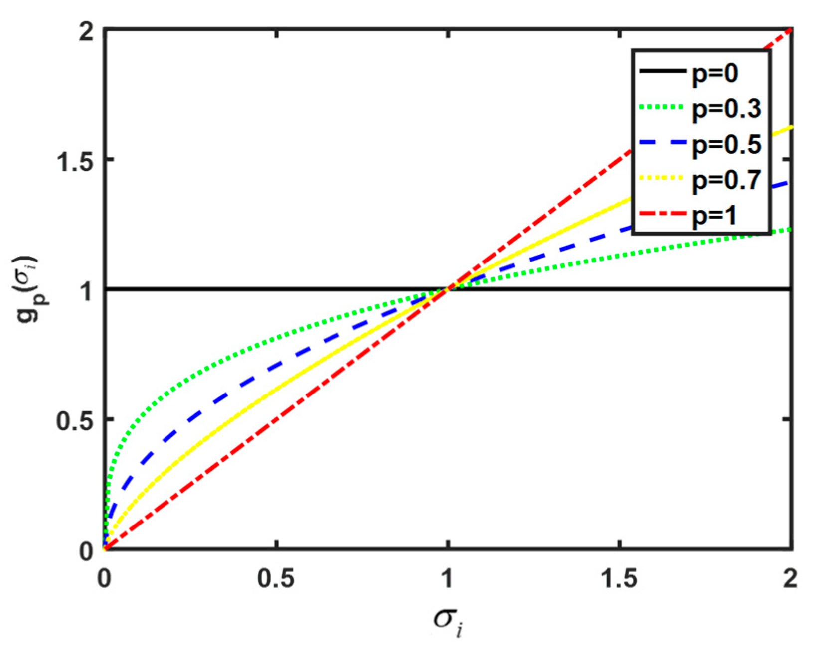Whether the low rank constraint form used can accurately perform convex approximation has a significant impact on the repair effect. Let ${‖\Phi X‖}_p={\displaystyle \sum _i^n{g}_p({\sigma }_i)}$, where function $g_p({\sigma }_i)={\sigma }_i^p , 0\le p\le 1$. For the $l_0$ and $l_{\mathrm{p}}$ norms, the function $g_p({\sigma }_i)$ is

$$g_0({\sigma }_i)=\left\{ \begin{array}{ll}0 ,& {\sigma }_i=0\\ 1 ,& {\sigma }_i\ne 0\end{array}\right.,g_1({\sigma }_i)={\sigma }_i.$$

Normalize ${\sigma }_i$ within the range of 0–1 and plot the curves of function $g_p({\sigma }_i)$ at p = 0, 0.3, 0.5, 0.7, and 1. A visualization of the convex approximation is shown in Figure 1. It can be seen that the smaller the value of p is, the closer the convex approximation function $g_p({\sigma }_i)$ curve is to the $l_0$ norm curve.

Figure 1. The curves of $g_p({\sigma }_i)$, where p = 0, 0.3, 0.5, 0.7, and 1.

As the simplest convex substitution of the $l_0$ norm, the nuclear norm is the most common in low-rank constraint modeling. To further improve the accuracy of low-rank approximation, we can use the weighted $l_1$ norm of the singular values of the matrix, that is, the weighted nuclear norm [29,30,31,32], or use the truncated nuclear norm [33,34,35,36] to replace the nuclear norm. Common regularization constraint schemes for low-rank matrices are summarized as follows.

2.1. Nuclear Norm ${‖X‖}_{*}$

For example, we use the minimized nuclear norm as a low-rank constraint to establish an image-inpainting model, as follows:

$$\begin{array}{l}\stackrel{\wedge }{X}=\arg \underset{X}{\min }{‖\Phi X‖}_{*}\\ s.t. Y-{\Theta }_{\Omega }X\le \epsilon \end{array}$$

(2)

where $Y$ is the impulse interference image of size $n_1\times n_2$. The regularization parameter $\lambda$ is introduced to convert model (2) into the following unconstrained form:

$$\stackrel{\wedge }{X}=\arg \underset{X}{\min }\frac{1}{2}{‖Y-{\Theta }_{\Omega }X‖}_F^2+\lambda {‖\Phi X‖}_{*}$$

(3)

Three algorithms can be used to solve Equation (3). The most commonly used algorithm is the singular value shrinkage/threshold (SVT) algorithm [37].

The SVT algorithm is shown below.

First, perform singular value decomposition for $Y$,$U\Sigma V^H=SVD\left(Y\right)$,$\Sigma =diag \left( {\left\{{\sigma }_i\right\}}_{1\le i\le n} \right)$, where $diag \left( . \right)$ is the diagonal matrix operation of the elements, $n=\min (n_1, n_2)$. Then, soft threshold operation $D_{\lambda }({\sigma }_i)= \max \left(0, {\sigma }_i-\lambda \right)$ is performed on the singular values [38]. Then, set ${\Sigma }_{SVT}=diag\left( {\{D_{\lambda }({\sigma }_i)\}}_{1\le i\le n} \right)$. Finally, obtain the solution results $\stackrel{\wedge }{X}=U{\Sigma }_{SVT}{V}^H$.

Jain P. proposed the singular value projection (SVP) algorithm in order to solve the problem in model (2) [39]. With the development of large-scale data processing and distributed computing, the alternating direction method of multipliers (ADMM) algorithm has become the mainstream optimization algorithm [40]. When using the ADMM algorithm to solve (3), auxiliary variables $Z=\Phi X$ and residuals $L$ must first be introduced to transform model (3) into multiple sub-problems for an iterative solution:

$$(\stackrel{\wedge }{X},\stackrel{\wedge }{Z},\stackrel{\wedge }{\Theta })=\arg \underset{x,z,\Theta }{\min }\frac{1}{2}{‖Y-{\Theta }_{\Omega }X‖}_F^2+\frac{\lambda }{2}{‖Z‖}_{*}+\frac{\lambda \rho }{2}{‖\Phi X-Z+\Theta ‖}_F^2$$

where $\rho >0$ is the introduced penalty parameter, and the SVT method is used to solve sub-problem $\stackrel{\wedge }{Z}$.

In this paper, we use the SVT algorithm, SVP algorithm, and ADMM algorithm to solve the nuclear-norm-based image-inpainting model, which correspond by name to the SVT method, SVP method, and n_ADMM method, respectively. The details of the SVT algorithm, SVP algorithm, and n_ADMM algorithm are shown in Algorithms 1–3, respectively.

Algorithm 1. The SVT algorithm for solving model (3)

Input: $Y, {\Theta }_{\Omega }, \rho ,\lambda$$, \mathrm{the} \mathrm{maximum} \mathrm{number} \mathrm{of} \mathrm{iterations} t_{\max }$$, \mathrm{convergence} \mathrm{condition} {\eta }_{tol}=e-6$.

Initialization: $(m,n)=size(Y)$$, X^{(0)}=zeros(m,n)$$, Y_d^{(0)}=Y$$, t=1$.

While $t<t_{\max }$$\mathrm{and} {\eta }^{(t)}<{\eta }_{tol}$ do

$[U,S,V]=SVD(Y_d^{(t-1)})$.

${\delta }_0=diag(S)$$, \tau =\raisebox{1ex}{$1$}\!\left/ \!\raisebox{-1ex}{$\rho $}\right.$$, \delta =1-\min (\raisebox{1ex}{$\tau $}\!\left/ \!\raisebox{-1ex}{${\delta }_0$}\right.,1)$$, {\delta }_0={\delta }_0*\delta$.

Update $X^{(t)}=\left|U*diag({\delta }_0)*V^H\right|$.

Update $Y_d^{(t)}=\left|Y_d^{(t-1)}+\lambda (Y-X^{(t)})\right|$.

Update ${\eta }^{(t)}=\frac{{‖\left|X^{(t)}\right|-\left|X^{(t-1)}\right|‖}_F}{{‖\left|X^{(t)}\right|‖}_F}$.

$t=t+1$.

End while

$X^{*}(i, j)=\left\{\begin{array}{l}{X}^{(t)}(i, j), (i, j)\in \Omega \\ Y(i, j),\hspace{1em} (i, j)\notin \Omega \end{array}\right.$.

Output: $X^{*}$.

Algorithm 2. The SVP algorithm for solving model (2)

Input: $Y, {\Theta }_{\Omega }, \tau =0.01$$, \mathrm{the} \mathrm{rank} r$$, \mathrm{the} \mathrm{maximum} \mathrm{number} \mathrm{of} \mathrm{iterations} t_{\max }$$, \mathrm{convergence} \mathrm{condition} {\eta }_{tol}=e-6$.

Initialization: $(m,n)=size(Y)$$, X^{(0)}=zeros(m,n)$$, Y_d^{(0)}=Y$$, t=1$.

While $t<t_{\max }$$\mathrm{and} {\eta }^{(t)}<{\eta }_{tol}$ do

$Y_d^{(t)}=X^{(t-1)}-\tau (X^{(t-1)}-Y)$.

${\Theta }_{\Omega }{Y}_d^{(t)}={\Theta }_{\Omega }Y$.

$[U,S,V]=SVD(Y_d^{(t)})$

${\delta }_0=diag(S)$$, {\delta }_0={\delta }_0(1:r,1)$.

Update $X^{(t)}=\left|U(:,1:r)*diag({\delta }_0)*V{(:,1:r)}^H\right|$.

Update ${\eta }^{(t)}=\frac{{‖\left|X^{(t)}\right|-\left|X^{(t-1)}\right|‖}_F}{{‖\left|X^{(t)}\right|‖}_F}$.

$X^{(t)}(i, j)=\left\{\begin{array}{l}{X}^{(t)}(i, j), (i, j)\in \Omega \\ Y(i, j), \hspace{1em}(i, j)\notin \Omega \end{array}\right.$$, t=t+1$.

End while

$X^{*}=X^{(t)}$.

Output: $X^{*}$.

Algorithm 3. The n_ADMM algorithm for solving model (3)

Input: $Y, {\Theta }_{\Omega }, \rho ,\lambda$$, \mathrm{the} \mathrm{maximum} \mathrm{number} \mathrm{of} \mathrm{iterations} t_{\max }$$, \mathrm{and} \mathrm{convergence} \mathrm{condition} {\eta }_{tol}=e-6$.

Initialization: $(m,n)=size(Y)$$, X^{(0)}=zeros(m,n)$$,Y_d^{(0)}=Y$$, Z^{(0)}=zeros(m,n)$$, L^{(0)}=zeros(m,n)$$, t=1$.

While $t<t_{\max }$$\mathrm{and} {\eta }^{(t)}<{\eta }_{tol}$ do

Update $X^{(t)}=(Y_d^{(t-1)}+\lambda \rho (Z^{(t-1)}-L^{(t-1)}))./({\Theta }_{\Omega }+\lambda \rho )$.

$[U,S,V]=SVD(X^{(t)}+L^{(t-1)})$.

${\delta }_0=diag(S)-\raisebox{1ex}{$1$}\!\left/ \!\raisebox{-1ex}{$\rho $}\right.$$, {\delta }_0(find({\delta }_0)<0)=0$.

Update $Z^{(t)}=U*diag({\delta }_0)*V^H$.

Update $L^{(t)}=L^{(t-1)}+X^{(t)}-Z^{(t)}$.

Update ${\eta }^{(t)}=\frac{{‖\left|X^{(t)}\right|-\left|X^{(t-1)}\right|‖}_F}{{‖\left|X^{(t)}\right|‖}_F}$.

$t=t+1$.

End while

$X^{*}(i, j)=\left\{\begin{array}{c}\left|X^{(t)}(i, j)\right|, (i, j)\in \Omega \\ Y(i, j), \hspace{1em}(i, j)\notin \Omega \end{array}\right.$.

Output: $X^{*}$.

2.2. Weighted Nuclear Norm ${\displaystyle \sum _{i}fun\left({\sigma }_i\right)}$

The weighted nuclear norm ${\displaystyle \sum _{i}fun\left({\sigma }_i\right)}$ is a scheme that uses weighted singular value constraints to approximate $l_0$ constrained singular values [29,30,31,32]. It is a balanced constraint scheme that makes large singular values smaller and small singular values larger. It can be more accurate than the nuclear norm (i.e., $l_1$ constraints on singular values), where $fun\left( . \right)$ is the weighted function of each singular value ${\sigma }_i$ of matrix $\Phi X$, and $[ U, diag{\left\{{\sigma }_i\right\}}_{i=1:\min (n_1,n_2)}, V ]=SVD(\Phi X)$. We use the weighted nuclear norm as a low-rank constraint to establish an image-inpainting model, as follows:

$$\begin{array}{l}\stackrel{\wedge }{X}=\arg \underset{X}{\min }{\displaystyle \sum _{i}fun\left({\sigma }_i\right)}\\ s.t. Y-{\Theta }_{\Omega }X\le \epsilon \end{array}$$

(4)

Then, we introduce the regularization parameter $\lambda$ and convert model (4) into an unconstrained form:

$$\stackrel{\wedge }{X}=\arg \underset{X}{\min }\frac{1}{2}{‖Y-{\Theta }_{\Omega }X‖}_F^2+\lambda {\displaystyle \sum _{i}fun\left({\sigma }_i\right)}$$

(5)

There are many kinds of weighting functions $fun\left( . \right)$, and the p-norm ($0 \text{<} \mathrm{p} \text{<} 1$) is the simplest weighting scheme, namely, $g_p({\sigma }_i)=fun\left({\sigma }_i\right)$. Reference [30] reviewed various weighting functions that approximate the $l_0$ norm of singular values, such as SCAD [41], MCP [42], Logarithm [43], Geman [44], Laplace [45,46], etc., among which the Logarithm scheme is the most classic. In the experimental section of this paper, we choose the Logarithm scheme to perform our comparisons. The weighting function in the Logarithm scheme is shown below:

$$fun\left({\sigma }_i\right) =\frac{\lambda }{\log (\gamma +1)}\log (\gamma {\sigma }_i+1)$$

(6)

where $\gamma >0$ is a parameter that is determined based on experience.

The simplest and most direct solution to model (4) is the weighted SVT (WSVT) algorithm. Set the weight $w_i=fun\left({\sigma }_i\right)$, $i=1,2,\dots ,n$, and then $\stackrel{\wedge }{X}=U{\Sigma }_{WSVT}{V}^H$, where ${\Sigma }_{WSVT}=diag\left({\{D_{\lambda }(w_i{\sigma }_i)\}}_{1\le i\le n}\right)$.

We use ADMM to solve the weighted nuclear norm image-inpainting problem (5). We introduce auxiliary variables $Z=\Phi X$ and residuals $L$ to transform model (5) into multiple sub-problems for iterative solution:

$$(\stackrel{\wedge }{X},\stackrel{\wedge }{Z},\stackrel{\wedge }{L})=\arg \underset{x,z,L}{\min }\frac{1}{2}{‖Y-{\Theta }_{\Omega }X‖}_F^2+\frac{\lambda }{2}{\displaystyle \sum _{i}fun\left({\sigma }_i\right)}+\frac{\lambda \rho }{2}{‖\Phi X-Z+L‖}_F^2$$

(7)

where $\rho >0$ is the introduced penalty parameter, and the WSVT algorithm is used to solve the sub-problem $\stackrel{\wedge }{Z}$. The combination of the weighted SVT algorithm and ADMM algorithm can obtain more accurate iterative estimations. We use the ADMM algorithm to solve the weighted-nuclear-norm-based image-inpainting model (7), and name it the WSVT_ADMM method. The details of the WSVT_ADMM algorithm used to solve model (7) are shown in Algorithm 4.

Algorithm 4. The WSVT_ADMM algorithm for solving model (7)

Input: $Y, {\Theta }_{\Omega }, \rho ,\theta ,\lambda ,\gamma$$, \mathrm{the} \mathrm{maximum} \mathrm{number} \mathrm{of} \mathrm{iterations} t_{\max }$$, \mathrm{decay} \mathrm{factor} \varsigma =0.9$ $\mathrm{convergence} \mathrm{condition} {\eta }_{tol}=e-6$.

Initialization: $(m,n)=size(Y)$$, X^{(0)}=zeros(m,n)$$, L^{(0)}=zeros(m,n)$$, Y_d^{(0)}=Y$$, \lambda =\varsigma *\max (\left|Y(:)\right|)$$, t=1$.

While $t<t_{\max }$$\mathrm{and} {\eta }^{(t)}<{\eta }_{tol}$ do

$[U,S,V]=SVD(Y_d^{(t-1)})$.

${\delta }_0=diag(S)$$, w=fun({\delta }_0,\gamma ,\lambda )$$, {\delta }_0={\delta }_0-w*\raisebox{1ex}{$1$}\!\left/ \!\raisebox{-1ex}{$\rho $}\right.$$, {\delta }_0(find({\delta }_0<0))=0$.

Update $X^{(t)}=U*diag({\delta }_0)*V^H$.

Update $Y_d^{(t)}=\left|Y_d^{(t-1)}+\theta (Y-X^{(t)})\right|$.

Update ${\eta }^{(t)}=\frac{{‖\left|X^{(t)}\right|-\left|X^{(t-1)}\right|‖}_F}{{‖\left|X^{(t)}\right|‖}_F}$.

$\lambda =\varsigma *\lambda$$, X^{(t)}(i, j)=\left\{\begin{array}{l}{X}^{(t)}(i, j), (i, j)\in \Omega \\ Y(i, j), \hspace{1em}(i, j)\notin \Omega \end{array}\right.$$, t=t+1$.

End while

$X^{*}=X^{(t)}$.

Output: $X^{*}$.

2.3. Truncated Nuclear Norm

In general, the singular value curve of a low-rank matrix exhibits an exponential extreme decay trend from large to small, and the singular values sorted backward will approach 0. Therefore, the minimization of the nuclear norm is mainly to constrain the minimization of large singular values. To fully utilize the small singular values, a truncated nuclear norm minimization scheme can be used. The purpose of truncated nuclear norm minimization is to constrain the minimization of small singular values [33,34,35,36]. We use the truncated nuclear norm as a low-rank constraint to establish an image-inpainting model, as follows:

$$\begin{array}{l}\stackrel{\wedge }{X}=\arg \underset{X}{\min } \Vert \Phi X{\Vert }_{\ast }-{\mathcal{T}}_r ( U^H\Phi XV ) \\ s.t. Y-{\Theta }_{\Omega }X\le \epsilon \end{array}$$

(8)

where ${\mathcal{T}}_r$ is a truncation operation that extracts the first r larger diagonal elements in the diagonal matrix $U^H\Phi XV$, and $\left|\right|\Phi X|{|}_{\ast }-{\mathcal{T}}_r ( U^H\Phi XV )$ means that the first r larger diagonal elements in diagonal matrix $U^H\Phi XV$ are zeroed and the last r smaller diagonal elements are retained. We introduce a regularization parameter $\lambda$ and convert (8) into an unconstrained form:

$$\stackrel{\wedge }{X}=\arg \underset{X}{\min } \frac{1}{2}{‖Y-{\Theta }_{\Omega }X‖}_F^2+\lambda \left( \left|\right|\Phi X|{|}_{\ast }-{\mathcal{T}}_r ( U^H\Phi XV ) \right)$$

(9)

where $U,V$ are the truncated left and right singular value vector group matrices of $\Phi X$. The essence of truncated nuclear norm minimization is to minimize the sum of smaller singular value elements of the constrained low-rank matrices.

The truncated-nuclear-norm-based model can be solved by the APGL or ADMM algorithms. This paper combines the ADMM algorithm with the SVT algorithm to solve the truncated-nuclear-norm-based image-inpainting model (9), and abbreviates it as the TSVT (truncated SVT) algorithm. The details of the TSVT algorithm used to solve model (9) are shown in Algorithm 5.

Algorithm 5. The TSVT algorithm for solving the model (9)

Input: $Y, {\Theta }_{\Omega }, \rho ,\lambda$$, \mathrm{the} \mathrm{maximum} \mathrm{number} \mathrm{of} \mathrm{iterations} t_{\max }$, the truncated rank $r$$, \mathrm{convergence} \mathrm{condition} {\eta }_{tol}=e-6$.

Initialization: $(m,n)=size(Y)$$,X^{(0)}=zeros(m,n)$$,Y_d^{(0)}=Y$$,Z^{(0)}=zeros(m,n)$$,L^{(0)}=zeros(m,n)$$,t=1$.

While $t<t_{\max }$$\mathrm{and} {\eta }^{(t)}<{\eta }_{tol}$ do

$\tau =\raisebox{1ex}{$1$}\!\left/ \!\raisebox{-1ex}{$\rho $}\right.$$, T=Z^{(t-1)}-\tau *L^{(t-1)}$$, [U,S,V]=SVD(T)$.

${\delta }_0=diag(S)$$, \delta =1-\min (\raisebox{1ex}{$\tau $}\!\left/ \!\raisebox{-1ex}{$\left|{\delta }_0\right|$}\right.,1)$$, {\delta }_0={\delta }_0*\delta$.

Update $X^{(t)}=U*diag({\delta }_0)*V^H$.

$[U_Z,S_Z,V_Z]=SVD(Z^{(t-1)})$$, B=U_Z(:,1:r){.}^H*V_Z(:,1:r)$.

Update $Z^{(t)}=X^{(t)}+\tau *(L^{(t-1)}+B)$$, {\Theta }_{\Omega }{Z}^{(t)}={\Theta }_{\Omega }Y$.

Update $L^{(t)}=L^{(t-1)}+\rho (X^{(t)}-Z^{(t)})$.

Update ${\eta }^{(t)}=\frac{{‖\left|X^{(t)}\right|-\left|X^{(t-1)}\right|‖}_F}{{‖\left|X^{(t)}\right|‖}_F}$.

$t=t+1$.

End while

$X^{*}(i, j)=\left\{\begin{array}{l}\left|X^{(t)}(i, j)\right|, (i, j)\in \Omega \\ Y(i, j), \hspace{1em}(i, j)\notin \Omega \end{array}\right.$.

Output: $X^{*}$.

2.4. The F Norm of UV Matrix Factorization

The process of solving the nuclear norm minimization problem involves time-consuming matrix singular value decomposition. Earlier, Srebro N. [47] proposed the property ${‖X‖}_{*}=\underset{U{V}^H=X}{\min }\frac{1}{2}\left( {‖U‖}_F^2+ {‖V‖}_F^2\right)$ and then proved it. Later, the F norm of UV matrix factorization was used instead of the nuclear norm in many applications to simplify the calculation time [1,48]. We use the minimized F norm of UV matrix factorization as a low-rank constraint to establish an image-inpainting model, as follows.

$$\begin{array}{l}\stackrel{\wedge }{X}=\arg \underset{X}{\min } \frac{1}{2} \left( {‖U‖}_F^2+ {‖V‖}_F^2 \right)\\ s.t. Y-{\Theta }_{\Omega }X\le \epsilon , U{V}^H=\Phi X\end{array}$$

(10)

Then, we introduce the regularization parameter $\lambda$ and penalty parameter $\rho >0$ to convert model (10) into an unconstrained form:

$$\stackrel{\wedge }{X}=\arg \underset{U{V}^T=\Phi X}{\min }\frac{1}{2}{‖{\Theta }_{\Omega }X-Y‖}_F^2+\frac{\lambda }{2}\left({‖U‖}_F^2+{‖V‖}_F^2\right)+\frac{\lambda \rho }{2}{‖\Phi X-U{V}^T+L‖}_F^2$$

(11)

where $L$ is the residual variable. The initial values of $U$ and $V$ can be initialized using the LMaFit method [2,49]. Model (11) is commonly solved using the ADMM algorithm, and we name it the UV_ADMM method. The details of the UV_ADMM algorithm are shown in Algorithm 6.

Algorithm 6. The UV_ ADMM algorithm for solving model (11)

Input: $Y, {\Theta }_{\Omega }, \rho ,\lambda$$, \mathrm{the} \mathrm{maximum} \mathrm{number} \mathrm{of} \mathrm{iterations} t_{\max }$$, \mathrm{convergence} \mathrm{condition} {\eta }_{tol}$.

Initialization: $U_n^{(0)}$ and $V_n^{(0)}$ by the LMaFit method [49], $(m,n)=size(Y)$$,X^{(0)}=zeros(m,n)$$,Y_d^{(0)}=Y$$,L^{(0)}=zeros(m,n)$$,t=1$.

While $t<t_{\max }$$\mathrm{and} \eta <{\eta }_{tol}$ do

Update $X^{(t)}=[Y^{(t)}+\lambda \rho *(U^{(t-1)}{V}^{(t-1)H}-L^{(t-1)})]./({\Theta }_{\Omega }+\lambda \rho )$.

Update $U^{(t)}=\rho *(X^{(t)}+L^{(t-1)})*V^{(t-1)}*inv(eye(r)+\rho V^{(t-1)}{V}^{(t-1)H})$.

Update $V^{(t)}=\rho *(X^{(t)}+L^{(t-1)})*U^{(t)}*inv(eye(r)+\rho U^{(t)H}{U}^{(t)})$.

Update $L^{(t)}=L^{(t-1)}+X^{(t)}-U^{(t)}{V}^{(t)H}$.

Update ${\eta }_{t+1}=\frac{{‖X_n^{t+1}(:)-X_n^t(:)‖}_F}{{‖X_n^t(:)‖}_F}$.

$t=t+1$.

End while

$X^{*}(i, j)=\left\{\begin{array}{l}\left|X^{(t)}(i, j)\right|, (i, j)\in \Omega \\ Y(i, j), \hspace{1em}(i, j)\notin \Omega \end{array}\right.$.

Output: $X^{*}$

Compared with the n_ADMM method, the F norm of the UV-matrix-based UV_ ADMM method avoids the time-consuming SVD in each iteration, making it more suitable for large matrix modeling with low-rank constraints. This method and the weighted nuclear norm method are commonly used in low-rank matrix constrained models. The above model and its solving algorithm are summarized in Table 1.

Table 1. Modeling and solving algorithms based on the low-rank constraint in this paper.

Constrained Modeling	Nuclear Norm	Truncated Nuclear Norm			Weighted Nuclear Norm	Matrix Decomposition F Norm
Solution algorithm	SVT	SVP	ADMM	ADMM	ADMM	ADMM
Method abbreviation	SVT	SVP	n_ADMM	TSVT_ADMM	WSVT_ADMM	UV_ADMM

In addition, other algorithms can solve the above model, for example, commonly used algorithms in sparsity-solving models. A sparse constraint on a signal refers to minimization of the l₀ norm of signal elements, while a low-rank constraint on a signal refers to minimization of zero norms of the singular value of the signal matrix. Therefore, the optimization solution based on a low-rank constraint model has a lot in common with the optimization solution based on the sparse constraint model in solving the algorithm. Iterative optimization algorithms based on sparse constraint models can be applied to optimization solutions based on matrix low-rank constraint models, such as convex relaxation algorithms, which find a sparse or low-rank approximation of signals by transforming nonconvex problems into convex problems through iterative solutions. Among them, the conjugate gradient (CG) algorithm, iterative soft thresholding (IST) algorithm [50], Split Bregman algorithm [51], and major minimize (MM) algorithm [52] can be flexibly changed according to different optimization models.

3. Comparative Experiments

In this section, we conduct a comparison of the above methods for solving satellite-image-inpainting problems. We simulated the impulse interference on satellite images with an interference rate of 30% (the interference rate is the percentage of interference pixels among the total number of image pixels). The three kinds of impulse interference were as follows: A. random impulse interference; B. salt and pepper impulse interference; C. and random missing pixels. The satellite images in this paper are sourced from the public dataset DOTA v.2.0 (https://captain-whu.github.io/DOTA/dataset.html, accessed on 12 December 2020), with images provided by the China Resources Satellite Data and Application Center, satellite GF-1, satellite GF-2, etc. The methods employed in the comparison are SVT, SVP, n_ADMM, TSVT_ADMM, WSVT_ADMM, and UV_ADMM. For a fair comparison, each method is carried out using its optimal parameters to ensure every method shows its most representative performance.

The relative least normalized error (RLNE) and the structural similarity (SSIM) [53] are used as image-inpainting quality indicators. The RLNE is an index based on the error between pixels, and the SSIM index is more consistent with human visual perception in image visual evaluation. Generally, the larger the SSIM value is, the better the image-inpainting quality is. All simulations were carried out on a Windows 10 operating system and MATLAB R2019a running on a PC with an Intel Core i7 CPU 2.8 GHz and 16 GB of memory.

A gray satellite image and its singular values curve are shown in Figure 2a and Figure 2b, respectively. The singular values of the image descend rapidly from large to small, and most of them tend to be zero. This indicates that the image has the characteristic of being low rank. The three examples of impulse interference satellite images are shown in Figure 3, where the original image is the image in Figure 2a. It can be seen that the 30% interference rate has caused obvious information loss on the building shape, layout, gray value shading, and other features in the original image.

Figure 2. A gray satellite image and its singular values curve. (a) The gray satellite image; (b) the singular values curve of image in (a).

Figure 3. The interference satellite image (interference rate 30%): (a) random impulse interference pattern; (b) salt and pepper impulse interference pattern; (c) random missing pixel pattern.

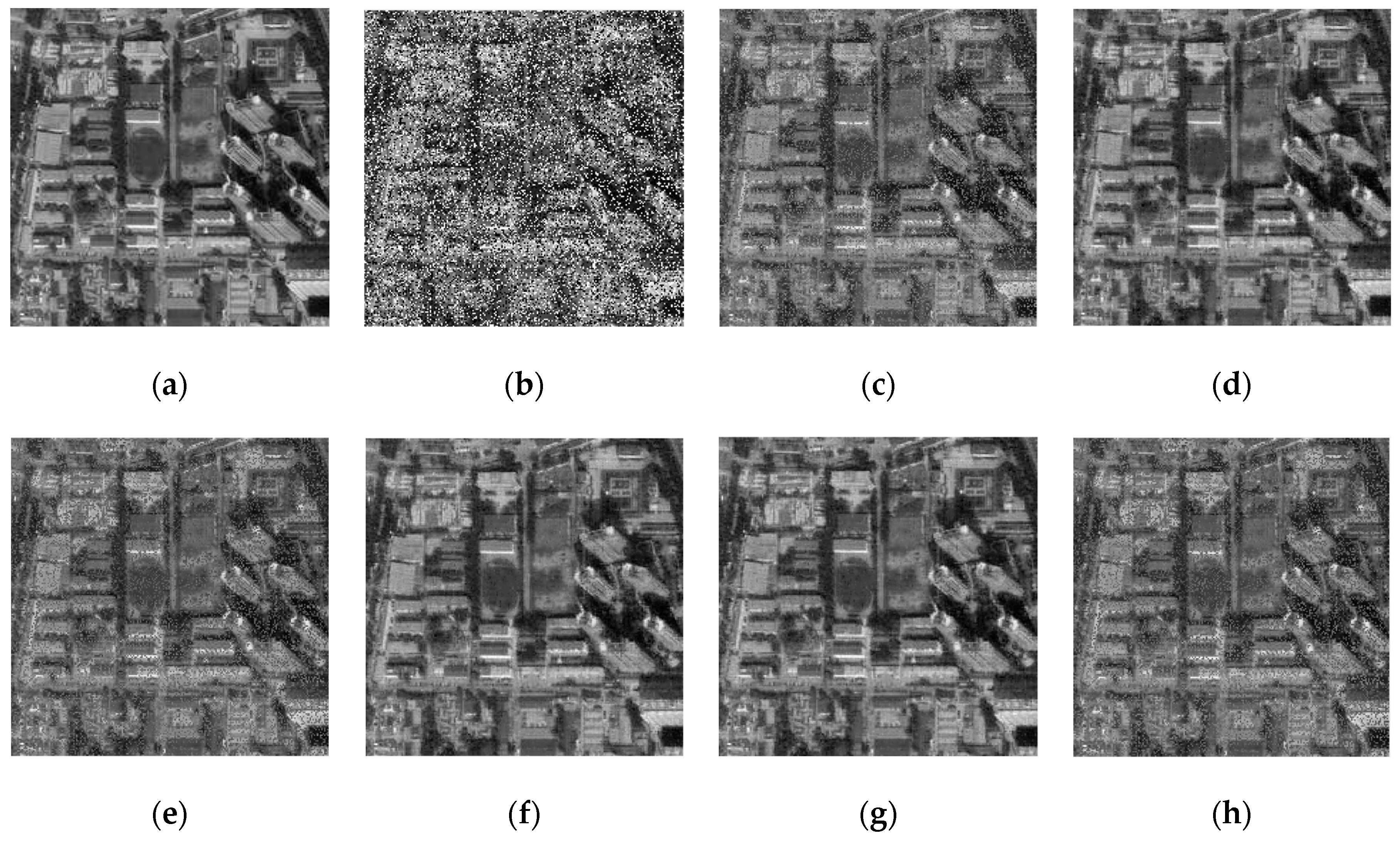
The comparison of the average values (RLNE, SSIM, and running time) of six image-inpainting methods under the interference of random impulse, salt and pepper noise, and missing pixels is shown in Table 2. The visual comparison of the six image-inpainting methods under the interference of salt and pepper noise is shown in Figure 4.

Table 2. Numerical comparison of six image-inpainting methods under three types of interference. (The bold indicators are the best indicators among various methods).

Noise Forms		Methods	Untreated	SVT	SVP	n_ADMM	TSVT_ ADMM	WSVT_ ADMM	UV_ ADMM
	Indices
Random impulse	RLNE (%)		45.88	18.36	9.83	19.70	8.43	8.19	20.01
	SSIM (%)		34.77	77.50	92.19	74.96	94.25	94.49	74.30
	Running time (s)		/	11.7357	0.5484	1.3883	1.0401	2.0523	0.3375
Salt and pepper noise	RLNE (%)		69.72	19.96	9.76	19.73	8.41	8.22	20.29
	SSIM (%)		18.63	74.18	92.25	74.79	94.21	94.39	73.80
	Running time(s)		/	5.34	0.4793	1.1451	1.2996	2.216	0.1993
Missing pixels	RLNE (%)		54.77	12.96	9.84	8.73	8.43	8.19	8.9
	SSIM (%)		32.46	87.91	92.25	94.02	94.25	94.49	93.69
	Running time (s)		/	9.9569	0.5418	0.5194	0.9842	2.3475	0.2543

Figure 4. Visual comparison of six image-inpainting methods under the interference of salt and pepper noise: (a) original image; (b) interference image; (c) SVT; (d) SVP; (e) n_ADMM; (f) TSVT_ADMM; (g) WSVT_ADMM; (h) UV_ADMM.

Based on the above visual and numerical comparison, we analyze the experimental methods below.

The matrix rank constraint method based on the F norm of UV matrix factorization (i.e., the UV_ADMM method) is equivalent to the method based on the nuclear norm constraint (i.e., the n_ADMM method) in terms of effectiveness. Overall, the n_ADMM method is slightly better, increasing the RLNE index by about 0.3% and the SSIM index by 0.3~1.

Since the nuclear-norm-based SVT, SVP, and n_ADMM methods, the weighted-nuclear-norm-based WSVT_ADMM method, and the truncated-nuclear-norm-based TSVT method all involve time-consuming SVD calculations in each iteration, the UV_ADMM method based on the UV matrix factorization F norm has significant advantages in terms of runtime. However, the UV_ADMM method did not achieve more accurate results compared to other methods, because the UV_ADMM method needs to initially set the estimated rank, for example, by using the LMaFit method to initialize the rank. However, the rank initialization is estimated and the accuracy of the rank is therefore not high, which leads to inaccurate low-rank constraints. Thus, this UV-matrix-factorization-based method is more commonly used for large-scale low-rank matrix calculations, and it can greatly reduce the inpainting time of large-scale matrix optimization as a result of avoiding the SVD of each iteration.

Since the weighted and truncated nuclear norm can better approach the singular value l₀ norm, the WSVT_ADMM and TSVT methods are significantly better than the nuclear-norm-based methods (SVT, SVP, n_ADMM) in terms of the accuracy of inpainting.

In summary, we have obtained a preliminary understanding that, in solving the same image restoration optimization problem using different algorithms, the various constraint schemes based on matrix low rank mentioned above can effectively solve the image optimization problem, but the solution accuracy and computation time vary. Compared to other schemes, weighted schemes can obtain more accurate repair results. In terms of computation time, because the time-consuming SVD decomposition is avoided, the matrix-factorization-based scheme saves more time compared to other schemes, but its repair accuracy is slightly lower than the weighted scheme, the truncated nuclear norm scheme, and the nuclear norm scheme. In addition, under the same low-rank constraint scheme of the matrix, using different algorithms to solve the problem also affects the accuracy of image restoration. For example, the nuclear norm scheme based on the SVP algorithm has a significantly better restoration accuracy than the nuclear norm scheme based on SVT, while the nuclear norm scheme based on the ADMM algorithm takes second place. It is obvious that the repair effects of the weighted nuclear norm scheme and truncated nuclear norm scheme are significantly better than that of the nuclear norm scheme.

4. Conclusions

In the application of machine vision, satellite images may suffer from three forms of impulse noise interference. In this paper, we use the low-rank characteristics of the image matrix to optimize and repair the images under three kinds of impulse interference and provide the optimization algorithm. Firstly, image-inpainting-modeling schemes based on nuclear norm, truncated nuclear norm, weighted nuclear norm, and matrix factorization F norm are reviewed. Then, the corresponding optimization iterative algorithms are provided, such as the TSVT_ ADMM algorithm, WSVT_ ADMM algorithm, UV_ ADMM algorithm, etc. Finally, the experimental results of various matrix-rank-constraint-based methods are presented visually and numerically, and a comparative analysis is provided. The experimental results show that all the mentioned matrix-rank-constraint-based methods can repair images to a certain extent and suppress certain forms of interference noise. Among the methods studied, those based on the weighted nuclear norm and the truncated nuclear norm achieved better repair effects, while methods based on the matrix factorization F norm take the shortest time and can be used for large-scale matrix low-rank calculation.