Underwater Image Enhancement Based on Difference Convolution and Gaussian Degradation URanker Loss Fine-Tuning

Abstract

Underwater images often suffer from degradation such as color distortion and blurring due to light absorption and scattering. It is essential to utilize underwater image enhancement (UIE) methods to acquire high-quality images. Convolutional networks are commonly used for UIE tasks, but their learning capacity is still underexplored. In this paper, a UIE network based on difference convolution is proposed. Difference convolution enables the model to better capture image gradients and edge information, thereby enhancing the network’s generalization capability. To further improve performance, attention-based fusion and normalization modules are incorporated into the model. Additionally, to mitigate the impact of the absence of authentic reference images in datasets, a URanker loss module based on Gaussian degradation is proposed during the fine-tuning. The input images are subjected to Gaussian degradation, and the image quality assessment model URanker is utilized to predict the scores of the enhanced images before and after degradation. The model is further fine-tuned using the score difference between the two. Extensive experimental results validate the outstanding performance of the proposed method in UIE tasks.

1. Introduction

Underwater images are crucial for advancing research in areas such as underwater biology and resource exploration. A clear underwater image can provide abundant underwater scene information for these tasks [1,2]. However, light scattering and absorption caused by marine microorganisms often lead to color distortion and blurring in underwater images [3]. As shown in Figure 1, the color distribution frequencies of different distorted images are imbalanced. Through underwater image enhancement (UIE) methods, the color distribution of the images is effectively balanced, significantly improving image quality. This is of great importance for researchers in the effective exploration of the ocean. These UIE methods are mainly categorized into visual prior-based methods, physical model-based methods, and deep learning-based methods. Visual prior-based methods enhance images by adjusting pixel values, yet they struggle to address complex underwater scenes due to the absence of constraints from underwater imaging models [4,5]. Physical model-based methods face challenges in estimating model parameters and suffer from the differences between underwater and terrestrial environments, making it difficult to construct models suitable for handling various distortions [6,7].

In recent years, convolutional network-based deep learning methods [8,9,10] have achieved significant performance in UIE tasks, owing to their exceptional robustness and stability. However, they still exhibit certain limitations. Most existing UIE methods [11,12] rely on classical convolution for feature extraction but do not incorporate prior knowledge. Since traditional convolutions start optimization from random initialization, they do not explicitly encode gradient information of the image [13]. This lack of explicit encoding makes it challenging during training to effectively extract edge gradient information, leading to potential loss of image detail information and subsequently limiting the model’s performance. To enhance model performance, researchers have incorporated additional image features as prior knowledge. For instance, Ucolor [9] uses extra-medium transmission as prior knowledge to improve the network’s response to degraded regions. WaterNet [8] integrates features from various preprocessed images to guide model training. However, these methods require additional datasets, such as high-quality medium transmission maps. Furthermore, to overcome the limited receptive fields of convolutional networks, researchers have introduced Transformer networks. For example, Peng et al. [14] proposed a Transformer-based U-shaped model that utilizes self-attention mechanisms to effectively capture long-range dependencies in images, thereby significantly improving model performance in UIE tasks. However, this approach also introduces complex training strategies and high computational costs.

Moreover, the training of these supervised network models often involves constraining the model’s convergence direction by predicting the feature distance between the image and a reference image, such as using ${\mathcal{L}}_1,{\mathcal{L}}_2$ loss, or perceptual loss [15] incorporating high-level semantic features. However, due to the intricate nature of underwater environments, distorted underwater image datasets lack authentic reference images. The reference images in current paired datasets are typically synthetically generated through existing methods and manually curated, leading to a degree of subjective interference in the model’s enhancement results. In response, researchers have also proposed the use of more effective loss functions for improvement. For example, Guo et al. [10] introduced the URanker loss into their enhancement network, using human perceptual factors to guide model convergence and reduce reliance on reference images. However, this approach only utilizes the URanker scores of the model’s enhanced images, which may result in ineffective constraints in the solution space.

To address these issues, we first propose a UIE network based on the difference convolution module. The introduction of difference convolution enables the module to effectively extract gradient and edge information, explicitly encoding prior knowledge into the convolutional neural network (CNN) and thereby enhancing the model’s ability to capture image features. Unlike existing UIE methods that incorporate prior knowledge, such as Ucolor and WaterNet, our difference convolution strategy does not rely on additional preprocessed dataset features. The difference convolution module consists of five distinct convolutions: Vanilla convolution, Center Difference Convolution (CDC), Angular Difference Convolution (ADC), Horizontal Difference Convolution (HDC), and Vertical Difference Convolution (VDC). Shallow features are crucial for the final enhancement results. Due to the differing receptive fields of shallow and deep features, direct addition does not effectively fuse them [16]. Therefore, we employ a channel-attention-based fusion module [17] that balances the impact of shallow and deep features by performing weighted multiplication followed by addition. Due to significant disparities in pixel value distributions across different channels in underwater images, we introduce a normalization module [5] at the end of the network to effectively handle pixel values exceeding a threshold. This approach enhances image quality further without introducing additional model parameters.

Additionally, to mitigate the impact of subjective factors from reference images in underwater image datasets on the results, we propose a Gaussian degradation-based URanker loss module during the fine-tuning phase. The Gaussian degradation operator introduces additional degradation to the input images, with its inherent randomness contributing to enhanced model robustness. URanker is a ranking-based underwater image quality assessment method, built upon an efficient conv-attentional image Transformer, whose predicted scores effectively evaluate the visual quality of images. Specifically, we apply the Gaussian degradation operator to the input images, then feed both the degraded and original images into the network to generate enhanced images. These images are evaluated using URanker to obtain quality scores, which are then used to fine-tune the network based on score differences. Unlike common supervised losses such as ${\mathcal{L}}_1$, this approach does not rely on reference image features. Compared to traditional unsupervised URanker loss, the introduction of enhanced image features from Gaussian-degraded inputs provides more effective constraints on the model’s solution space, further improving the model’s performance. Notably, the Gaussian degradation-based URanker loss is an unsupervised loss function. Its fine-tuning strategy enhances the model’s generalization without full retraining.

In summary, our contributions are as follows:

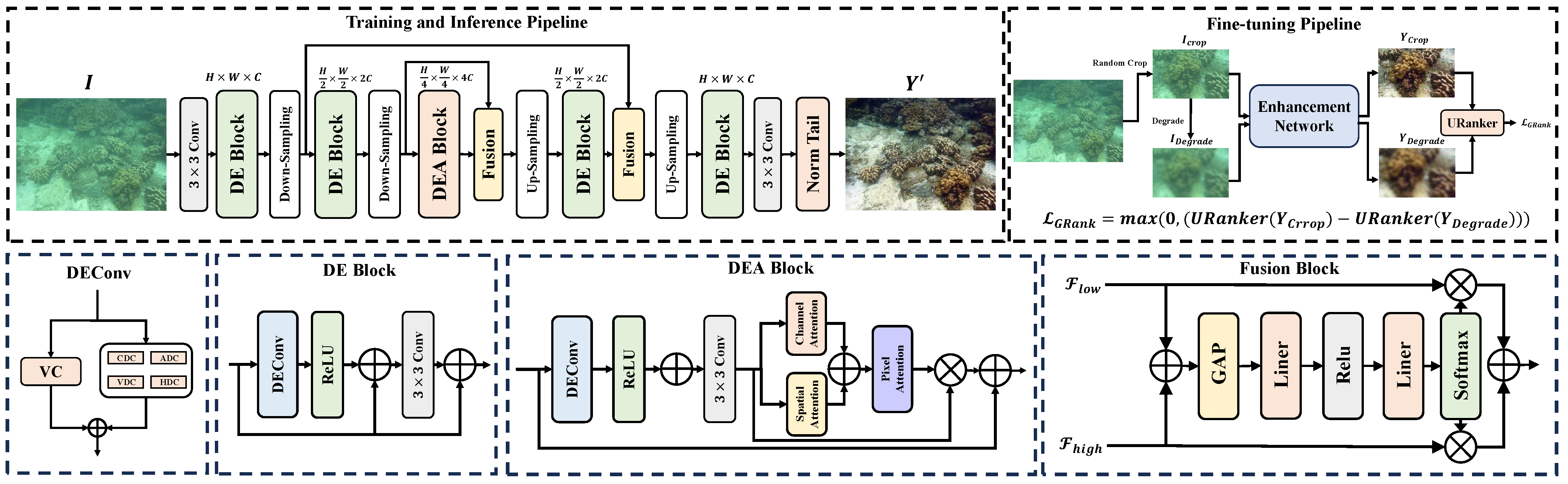
• We introduce a difference convolution module into the UIE network. Difference convolution effectively extracts image gradients and edge information, complementing vanilla convolution and thereby enhancing both the detail quality of the enhanced images and the overall performance of the model.
• We introduce a Gaussian degradation-based URanker loss module during the fine-tuning stage. This module guides model convergence by leveraging the URanker score differences between the enhanced results of original and Gaussian-degraded images, which further improves image quality and model generalization.
• Extensive experiments show that our method has better performance on different test datasets compared to other UIE methods.

2. Related Work

2.1. Underwater Image Enhancement

In recent years, underwater image enhancement has attracted increasing attention and research from scholars. Existing UIE methods can be categorized into three main types: visual prior-based methods [4,5], physical model-based methods [6,18,19], and deep learning-based methods [20,21]. Visual prior-based methods mainly adjust the pixel values of an image from the perspectives of contrast, brightness, and saturation to improve the image quality, such as histogram equalization [4] and white balance methods [5]. However, these methods do not account for the physical degradation process of underwater images, which can lead to over-enhancement. Physical model-based UIE methods mainly obtain enhanced images by solving the inverse of the physical model, such as in Dark Channel Prior (DCP) [6] and its variants (UDCP) [18]. Although these methods are theoretically robust, the complexity of underwater environments makes it challenging to adapt the assumed models to different types of underwater conditions. Moreover, accurately estimating numerous parameters poses a significant challenge, complicating the development of effective models. With the rapid development of deep learning, deep learning-based UIE methods have become a mainstream research direction. These methods primarily include CNN-based methods [8,10,22,23], GAN-based methods [11,24,25], and a few Transformer-based [14] methods. Li et al. [8] introduced WaterNet, a gated fusion convolutional network that takes the original image and three preprocessed versions as input, and ultimately fuses these inputs with predicted confidence maps to produce enhanced results. Qian et al. [22] proposed a hybrid algorithm model, HA-Net, which enhances the color and texture of underwater images through a dynamic color correction module based on depth estimation, a multi-scale U-Net structure, and global information compensation. Guo et al. [10] incorporated the pre-trained URanker into the NU2Net model as an additional supervision loss module, further enhancing model performance. Fu et al. [23] proposed PUIE-Net, a novel probabilistic network for UIE, by decomposing UIE into distribution estimation and consensus processes. This approach partially addresses the bias introduced by reference image labeling. Zhou et al. [26] proposed HCLR-Net, which enhances underwater image quality and model generalization by leveraging a hybrid contrastive learning regularization strategy and a unique negative sample construction method. Islam et al. [11] proposed a simple U-Net architecture, FUnIE-GAN, based on conditional GAN for UIE. Yan et al. [24] leveraged the powerful capabilities of CycleGAN combined with a physics-driven strategy to enhance the perceptual quality of underwater images. Chang et al. [25] proposed a UIE method based on a generative adversarial network, embedding a channel attention mechanism into the U-Net structure and integrating multiple loss functions for model training, effectively enhancing image quality. Cong et al. [27] proposed PUGAN, a physical-model-guided GAN method that enhances underwater image quality by combining parameter estimation with two-stream interaction enhancement subnets. Peng et al. [14] proposed the Transformer-based U-shape model in the field of UIE. By incorporating Transformer-based channel and spatial attention modules, they achieved significant improvements in image quality. Although the aforementioned UIE methods have demonstrated good performance, there is still room for improvement. Traditional CNN-based UIE methods require further enhancement in texture feature extraction. While incorporating prior knowledge can improve image quality, it also introduces the inconvenience of needing additional preprocessed datasets. Meanwhile, GAN-based approaches often face issues with training instability and convergence difficulties. Transformer-based methods enhance feature extraction but increase the number of model parameters. Furthermore, most methods’ loss functions overly rely on pseudo-reference images, while introducing unsupervised losses like URanker lacks sufficient solution space constraints. Therefore, we rethink the limitations of vanilla convolution in UIE methods and propose a novel convolution operator by integrating well-designed priors into the CNN to enhance feature learning capabilities. Additionally, we improve the model’s generalization ability by designing more effective constraint conditions.

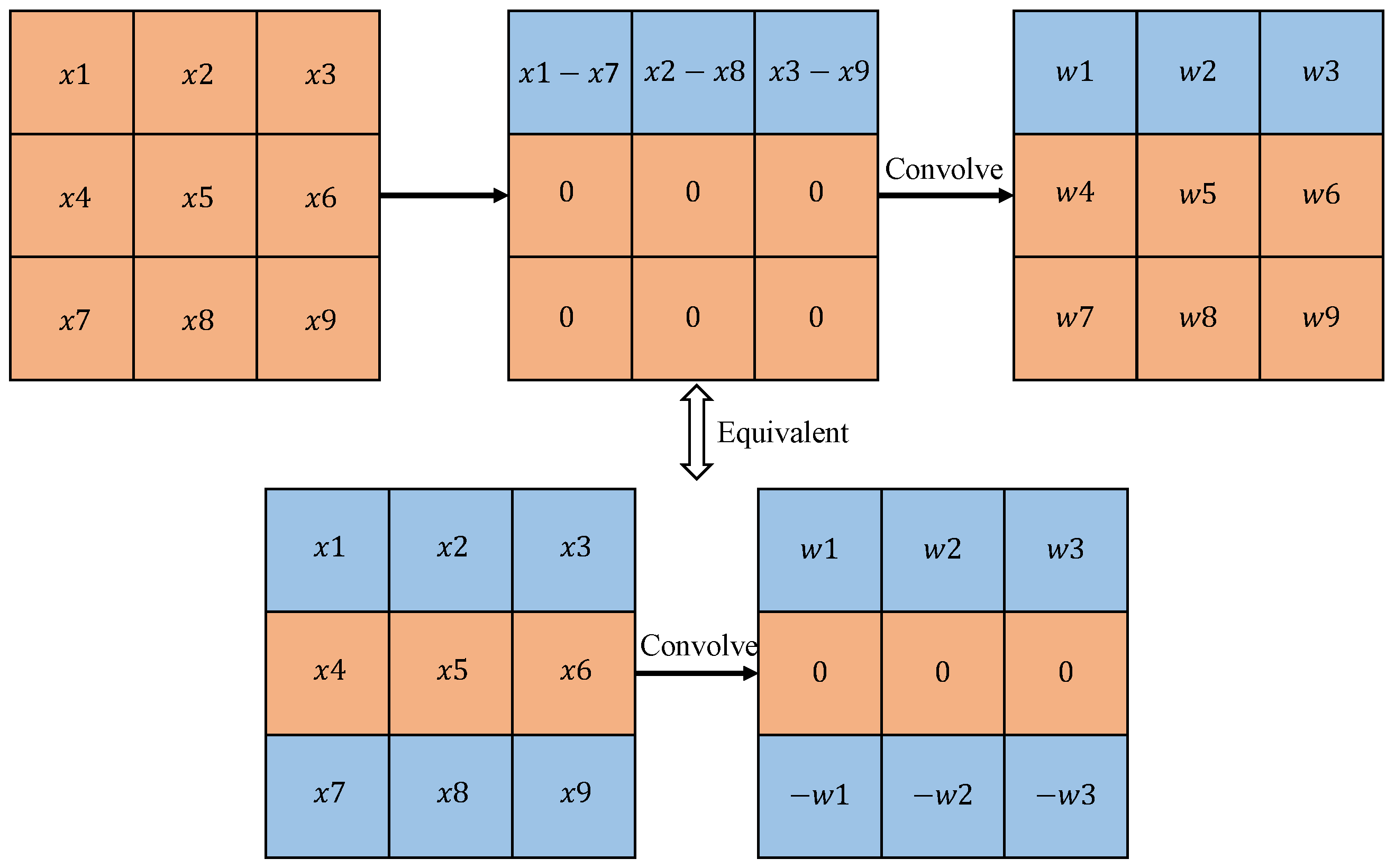
2.2. Difference Convolution

Difference convolution first appeared in Local Binary Patterns (LBPs) proposed by Oulu. It involves comparing adjacent pixel values with the central pixel value and encoding these differences to reflect the texture information of the region [28]. Due to the tremendous success of convolutional network architectures in computer vision, various difference convolution modules have been proposed [29,30,31]. Inspired by LBP, Yu et al. [30] proposed Central Difference Convolution (CDC) for face detection tasks, which captures image details by aggregating intensity and gradient information. Subsequently, recognizing the redundancy in applying differential operations to all neighboring features with CDC, Yu et al. [31] introduced Cross-Central Difference Convolution, which decomposes CDC into two symmetric cross-operators: horizontal–vertical and diagonal. To integrate differential operations more efficiently into CNNs, Su et al. [32] introduced Pixel Difference Convolution, which first computes pixel differences in the image and then convolves these differences with kernel weights to produce output features. In recent research, Chen et al. [13] introduced difference convolution to image dehazing for the first time. They employed difference convolution to integrate prior knowledge, complementing standard convolution and enhancing the model’s representational capability. Inspired by this, we incorporated difference convolution into UIE tasks, further improving the performance of the enhancement network.

3. Method

As shown in Figure 2, our method consists of two main stages. In the training phase, a difference convolution-based U-Net architecture is proposed, which includes an encoder, a decoder, and a channel-attention-based feature fusion module, with results produced by a normalization module at the end. In the fine-tuning phase, a Gaussian degradation-based URanker loss module is introduced. The input image is first degraded using a degradation operator. Both the degraded image and the original image are then fed into the enhancement network. The difference in URanker scores between the enhanced images is used to further refine the model training.

3.1. Difference Convolution Module

In the field of UIE, previous methods typically employed vanilla convolutional modules for feature extraction [8,9,33]. Since vanilla convolutions are optimized starting from random initialization during training, it is difficult to effectively extract edge gradient information, thus limiting the model’s performance. Due to light attenuation and scattering, underwater images frequently display color distortion (bluish or greenish) and blurred details, leading to a noticeable loss of both low-frequency and high-frequency information in the images. It is generally noted that low-frequency information plays a critical role in color distribution, while high-frequency information such as gradient edges is also essential in recovering image details. However, vanilla convolution (VC) often tends to capture low-frequency information while neglecting high-frequency details in feature extraction [13]. Previous work has approached this challenge by integrating prior knowledge [9,34,35] to improve the restoration of high-frequency information in images. Inspired by these approaches, we designed a network module based on difference convolution. By combining different difference convolution modules with vanilla convolution in parallel, we introduce well-designed priors to the convolutional layers, enabling the model to effectively capture both low-frequency and high-frequency information in the image. As illustrated in the training phase of Figure 2, the network’s Difference Enhanced Convolution (DEConv) is constructed by arranging four difference convolutions (DC) alongside one vanilla convolution. The four DCs are Central Difference Convolution (CDC), Angular Difference Convolution (ADC), Horizontal Difference Convolution (HDC), and Vertical Difference Convolution (VDC). In DCs, prior information is typically encoded into convolutional neural networks using a pixel-pair difference calculation strategy. HDC and VDC further incorporate traditional local descriptors (such as Sobel [36] or Scharr [37]) into the convolutional layers. For instance, in VDC as shown in Figure 3, vertical gradients are initially extracted by computing the differences between selected pixel pairs, which are then multiplied by the convolutional kernel. After training, the learned kernel weights are reordered to an equivalent format, and convolution is directly applied to the untouched input features. Notably, the reordered convolutional kernel resembles traditional vertical convolution kernels (such as Sobel [36] and Scharr [37]), where the sum of the vertical weights is zero. The derivation of HDC follows a similar reasoning. This equivalent reordering allows the learned convolutional kernel to effectively capture gradient information within the image, thereby enhancing the model’s performance.

By combining the features learned from DCs and VC, our module more effectively extracts both high-frequency and low-frequency features from the image. As shown in Figure 4, the application of DCs results in clearer texture details in the image. Building upon the DEConv module, the Difference Enhanced (DE) block and the Difference Enhanced Attention (DEA) block are subsequently introduced. The DE Block consists of a DEConv layer, a ReLU activation layer, and a $3\times 3$ convolution layer, which effectively mitigates the vanishing gradient problem through residual connections. The DEA Block extends the DE Block by integrating channel attention, spatial attention, and pixel attention mechanisms [38,39]. By combining these attention mechanisms, the DEA Block guides the model to focus on important parts of features across different channels, thereby highlighting useful feature information and improving network performance. From the model framework diagram, it can be observed that our model adopts a three-layer encoder–decoder structure based on U-Net. The encoder–decoder structures of the first and second layers use DE Blocks, while the third layer utilizes DEA Blocks. The dimensional sizes of level 1, level 2, and level 3 are $C\times H\times W$, $2C\times {\displaystyle \frac{H}{2}}\times {\displaystyle \frac{W}{2}}$, and $4C\times {\displaystyle \frac{H}{4}}\times {\displaystyle \frac{W}{4}}$, respectively. In our implementation, we set the value of C to 32. The DE Block in the decoder enhances the model’s ability to reconstruct detailed features of the image. As shown in Figure 5, during the upsampling process in the decoder stages, the feature maps progressively increase in size, enhancing the recovery of image details.

3.2. Fusion and Normalization Modules

Shallow features play a significant role in enhancing underwater images. Many U-Net-based models typically use direct addition to combine shallow and deep features [11,12]. However, due to the considerable difference in receptive fields and feature encoding between shallow and deep layers, direct addition does not effectively integrate these features. Inspired by [38], we adopt a feature fusion module based on channel attention mechanisms. For the input shallow features $F_{low}$ and deep features $F_{high}$, we employ global average pooling (GAP), a multi-layer perceptron (MLP) with a Linear–ReLU–Linear structure $F_{MLP}$, a softmax function, and a split operation to obtain the weights for both feature sets:

$$\left\{a_1,a_2\right\}=Split\left(Softmax\left(F_{MLP}\left(GAP(F_{low}+F_{high})\right)\right)\right)$$

(1)

Using the weights $a_1,a_2$ to fuse the shallow and deep features, the final output is obtained as follows:

$$y=a_1{F}_{low}+a_2{F}_{high}$$

(2)

At the end of the model, inspired by [10], we introduce a normalization tail to handle overflow values outside the range $[0,1]$. When overflow values are present in a channel $c\in \left\{r,g,b\right\}$, they can be represented as follows:

$$Y^{\prime }={\displaystyle \frac{Y_c^{\prime }-min\left(Y_c^{\prime }\right)}{max\left(Y_c^{\prime }\right)-min\left(Y_c^{\prime }\right)}}$$

(3)

where $Y_c^{\prime }$ denotes the values of the individual color channels, and $Y^{\prime }$ represents the final predicted image after normalization. It can effectively improve model performance without introducing additional parameters.

3.3. Gaussian Degradation-Based URanker Loss Module

Existing supervised models primarily use loss functions based on the difference between the predicted image and the target image for backpropagation, thereby constraining the model’s convergence [8,9]. However, due to the unique characteristics of underwater environments, current underwater reference images are often synthetically generated, leading to a degree of subjectivity in the quality of the images. To mitigate the impact of subjectivity on enhancement results, we propose a Gaussian degradation-based URanker loss module during the fine-tuning phase. Similar to the previous approach [10], the proposed method does not rely on reference image features and uses an unsupervised loss. The difference is that it simultaneously utilizes features from both the original input image and the degraded image, providing more effective constraints for the model’s solution space by incorporating additional perceptual scores from the degraded image. As illustrated in Figure 2, during the fine-tuning phase, a $64\times 64$ patch $I_{Crop}$ is randomly cropped from the input image I. A Gaussian degradation operator is then applied to further blur and reduce the image quality, resulting in $I_{Degrade}$. The images $I_{Crop},I_{Degrade}$ are input into the enhancement network to obtain $Y_{Crop}$ and $Y_{Degrade}$, respectively. These results are then fed into the URanker model to compute the score difference between them. Since Gaussian degradation further exacerbates information loss, the enhancement network faces a greater challenge in restoring such samples, and the URanker score for the enhanced results is generally lower. After initial training, the model can handle most common distorted images. Therefore, we use the enhanced result of the original input $Y_{Crop}$ as a pseudo-reference to guide the feature convergence of $I_{Degrade}$. The final unsupervised loss function is defined as follows:

$${\mathcal{L}}_{GRank}=max\left(0,\left(\mathrm{URanker}\left(Y_{Crop}\right)-\mathrm{URanker}\left(Y_{Degrade}\right)\right)\right)$$

(4)

The difference in scores between the two images reflects the disparity in their perceptual quality. If the score for the enhancement results of the degraded image is lower than that of the original input, it suggests that further optimization of the model is necessary, otherwise, the loss is considered to be zero.

3.4. Loss Function

During the training phase, the loss function of our model is primarily composed of the ${\mathcal{L}}_1$ loss and the contrastive loss [40]. The ${\mathcal{L}}_1$ loss trains the network by minimizing the pixel-wise difference between the predicted enhanced image $Y’$ and the corresponding reference image Y. Additionally, to further leverage the features of the original distorted image, we employ a contrastive loss. This loss function minimizes the distance between the predicted image and the reference image, while simultaneously maximizing the distance between the predicted image and the input image. This approach effectively directs the model’s convergence, ensuring that the high-level semantic features of the enhanced image align with those of the reference image, thereby enhancing the visual quality of the results. The final loss function is defined as follows:

$${\mathcal{L}}_1=∥Y^{\prime }-Y∥$$

(5)

$${\mathcal{L}}_{cr}=\sum _i^n{w}_i·{\displaystyle \frac{{∥F_i\left(Y\right)-F_i\left(Y^{\prime }\right)∥}_1}{{∥F_i\left(I\right)-F_i\left(Y^{\prime }\right)∥}_1}}$$

(6)

$${\mathcal{L}}_{total}={\lambda }_1{\mathcal{L}}_1+{\lambda }_2{\mathcal{L}}_{cr}$$

(7)

Here, I, $Y^{\prime }$, and Y represent the input image, predicted image, and reference image, respectively. $F_i(·)$ denotes high-level features extracted from various pre-trained layers of VGG-19, while $w_i$ represents a set of hyperparameters. Following the method in [40], features from the 1st, 3rd, 5th, 9th, and 13th layers of the pre-trained VGG-19 network are extracted, with corresponding weights $w_i$ ($i=1,2,3,4,5$) set to ${\displaystyle \frac{1}{32}},{\displaystyle \frac{1}{16}},{\displaystyle \frac{1}{8}},{\displaystyle \frac{1}{4}}$, and 1, respectively. ${\lambda }_1$ and ${\lambda }_2$ are hyperparameters used to adjust the weights of different losses, and are set to 1 and 0.25, respectively.

During the fine-tuning phase, to further constrain the model’s convergence, we remove the contrastive loss and introduce our proposed unsupervised loss module. The loss function is defined as follows:

$${\mathcal{L}}_{Finetune}={\lambda }_1{\mathcal{L}}_1+{\lambda }_3{\mathcal{L}}_{GRank}$$

(8)

The hyperparameters ${\lambda }_1$ and ${\lambda }_3$ are set to 1 and 0.5, respectively.

4. Experiment and Analysis

4.1. Datasets and Metrics

We utilized multiple real underwater image datasets to train and validate our model, including the UIEB [8], U45 [41], and SQUID [42] datasets. UIEB comprises 890 pairs of images with reference and 60 images without reference, covering various real underwater scenes. The 60 images without reference are selected from more complex and variable underwater environments, exhibiting severe color distortions. We chose 800 pairs for the training set, with the remaining 90 pairs and 60 challenging images designated as the test sets U90 and C60. Additionally, to further assess the robustness of our model, we used U45 and SQUID as test sets. U45 consists of 45 images that encompass various scenarios such as color shifts, low contrast, and haze-like blurring. The SQUID dataset contains 57 underwater stereo pairs captured from four different dive sites in Israel. Similar to [9], we selected 16 representative examples as the test set. For the test set U90, we assess the enhancement performance of the underwater images using full-reference image quality metrics, including peak signal-to-noise ratio (PSNR), Structure Similarity Index (SSIM), and Learned Perceptual Image Patch Similarity (LPIPS) [43]. In contrast, for the test sets C60, U45, and SQUID, we evaluate the model’s performance using no-reference image quality metrics, specifically Underwater Image Quality Measurement (UIQM) [44] and Underwater Color Image Quality Evaluation (UCIQE) [45]. PSNR and SSIM indicate how closely the results match the reference image in terms of image content or structure, while LPIPS provides a measure of similarity that aligns more closely with human perceptual responses. UIQM better reflects human perception of image quality by leveraging the specific degradation mechanisms and imaging characteristics of underwater environments. It is a linear combination of the Underwater Image Colorfulness Measure (UICM), the Underwater Image Sharpness Measure (UISM), and the Underwater Image Contrast Measure (UIConM). Specifically, UIQM can be expressed as $UIQM={\omega }_1\times UICM+{\omega }_2\times UISM+{\omega }_3\times UIConM$, where the weights ${\omega }_1=0.0282$, ${\omega }_2=0.2953$, and ${\omega }_3=3.5753$. UCIQE evaluates the quality of underwater images through a linear combination of chroma, saturation, and contrast. Specifically, UCIQE can be expressed as $UCIQE=c_1·{\sigma }_c+c_2·co{n}_l+c_3·{\mu }_s$, where $c_1=0.4680$, $c_2=0.2745$, and $c_3=0.2576$. Here, ${\sigma }_c$ represents the standard deviation of chroma, $co{n}_l$ represents the luminance contrast, and ${\mu }_s$ represents the mean saturation. A higher UCIQE value indicates better detail and clarity in the image.

4.2. Implementations

All experiments were conducted on the Ubuntu 20 operating system using the PyTorch framework, with an NVIDIA TITAN RTX GPU used for training and testing the UIE network. The model’s layer configuration was set to $[4,4,8,4,4]$ for $[N1,N2,N3,N4,N5]$, respectively. For training, we employed the Adam optimizer with parameters ${\beta }_1=0.9$, ${\beta }_2=0.999$, and $\epsilon =1\times {10}^{-8}$. The learning rate was initialized at $1\times {10}^{-4}$ and adjusted using a cosine annealing strategy to decay from the initial value to $1\times {10}^{-6}$. The batch size was set to 16, and the model was trained for 1000 epochs. For fair comparison, all deep learning-based UIE methods were trained on the same devices and datasets. In our experiment, the input images were uniformly cropped to a size of $256\times 256$, and data augmentation was applied using random flipping. During the fine-tuning phase, we used the same dataset as in the training phase, but without the need for corresponding reference images. For the input images, we randomly cropped them into 64 × 64 patches and applied data augmentation techniques, including vertical and horizontal flipping. The learning rate was set to $1\times {10}^{-7}$, and the model was trained for 80 epochs.

4.3. Quantitative Comparisons

To validate the performance and advantages of the proposed model, we conducted comparative experiments with twelve existing underwater image enhancement models. These methods are categorized into traditional and deep learning methods: the traditional methods include UDCP [18], IBLA [46], and MLLE [47]; the deep learning methods include WaterNet [8], FUnIE [11], Shallow-UWnet [12], Ucolor [9], PUIE-Net [23], U-shape [14], PUGAN [27], NU2Net [10], and HCLR-Net [26]. First, we conducted comparative experiments on the reference test set U90 to evaluate our method’s effectiveness in addressing underwater image distortions. The experimental results are presented in

Table 1. Quantitative comparison between different UIE methods on U90 test set. The top three results are marked with red, blue, and green, respectively. ↑ indicates that a higher value is better. ↓ indicates that a lower value is better.

Method	PSNR ↑	SSIM ↑	LPIPS ↓
UDCP (ICCVW’13)	10.277	0.486	0.392
IBLA (TIP’17)	15.046	0.683	0.316
WaterNet (TIP’19)	20.998	0.919	0.149
FUnIE (RAL’20)	19.454	0.871	0.175
Shallow-UWnet (AAAI’21)	18.120	0.721	0.289
Ucolor (TIP’21)	20.730	0.900	0.165
MLLE (TIP’22)	18.977	0.841	0.275
PUIE-Net (ECCV’22)	21.970	0.890	0.155
U-shape (TIP’23)	20.920	0.853	0.206
PUGAN (TIP’23)	22.576	0.920	0.159
NU2Net (AAAI’23, Oral)	22.669	0.924	0.154
HCLR-Net (IJCV’24)	23.667	0.932	0.136
Ours	23.436	0.935	0.125

. It can be observed that traditional methods based on physical models, such as UDCP and IBLA, perform worse in terms of enhancement metrics compared to deep learning-based methods. This discrepancy is likely due to the challenges in modeling physical phenomena, which impedes their ability to consistently handle diverse underwater scenarios. In contrast, deep learning-based approaches generally perform better, with recent methods like U-shape, NU2Net and HCLR-Net showing strong results. However, our proposed method outperforms these methods in several aspects. Specifically, compared to the state-of-the-art method HCLR-Net, although our PSNR is slightly lower, we achieve the second-best performance, with a 0.022 improvement in SSIM and a 0.011 reduction in LPIPS (lower LPIPS indicates better performance).

Additionally, the performance of different methods is evaluated on the no-reference datasets U45, SQUID, and C60. The experimental results are shown in

Table 2. Quantitative comparison of different UIE methods for the non-reference test sets U45, SQUID, and C60. The top three results are marked with red, blue, and green, respectively. ↑ indicates that a higher value is better. ↓ indicates that a lower value is better.

Method	U45		SQUID		C60
	UCIQE↑	UIQM↑	UCIQE↑	UIQM↑	UCIQE↑	UIQM↑
UDCP (ICCVW’13)	0.584	2.086	0.554	1.082	0.515	1.215
IBLA (TIP’17)	0.579	1.672	0.466	0.866	0.564	1.893
WaterNet (TIP’19)	0.582	3.295	0.571	2.518	0.566	2.653
FUnIE (RAL’20)	0.599	3.398	0.532	2.746	0.570	3.258
Shallow-UWnet (AAAI’21)	0.471	3.033	0.421	2.094	0.466	2.396
Ucolor (TIP’21)	0.564	3.351	0.514	2.215	0.532	2.746
MLLE (TIP’22)	0.598	2.599	0.562	2.314	0.581	2.310
PUIE-Net (ECCV’22)	0.578	3.199	0.522	2.323	0.558	2.521
U-shape (TIP’23)	0.553	3.248	0.528	2.256	0.534	2.783
PUGAN (TIP’23)	0.599	3.395	0.566	2.399	0.612	3.001
NU2Net (AAAI’23, Oral)	0.595	3.396	0.551	2.480	0.564	2.900
HCLR-Net (IJCV’24)	0.610	3.301	0.564	2.169	0.571	2.739
Ours	0.601	3.354	0.578	2.274	0.571	2.827

, and it can be found that our method achieves the best UCIQE metrics in the SUIQD dataset, and the second best UCQIE metrics in the U45 dataset. The UIQM metrics for our method are slightly lower compared to the best-performing methods. To provide a more detailed comparison of the performance of different methods on each image in the non-reference test set, we selected several methods that demonstrated superior performance and compared their UIQM and UCIQE values. The results are shown in Figure 6. It can be observed that the images enhanced by the proposed method generally exhibit favorable UIQM and UCIQE values across different test sets. For example, the proposed method shows promising performance in terms of UCIQE on the SQUID dataset. Although its performance is somewhat weaker on certain datasets, it still maintains an overall favorable level across multiple datasets. This suggests that the proposed method demonstrates a certain degree of stability across different image scenarios. Since UCIQE and UIQM are biased towards specific features rather than evaluating the entire image and do not account for color shifts and artifacts, some excessively enhanced underwater images may still achieve high scores [8]. Therefore, these metrics may not always provide an accurate reflection of model performance. A comprehensive evaluation should incorporate both qualitative and quantitative methods to address this issue.

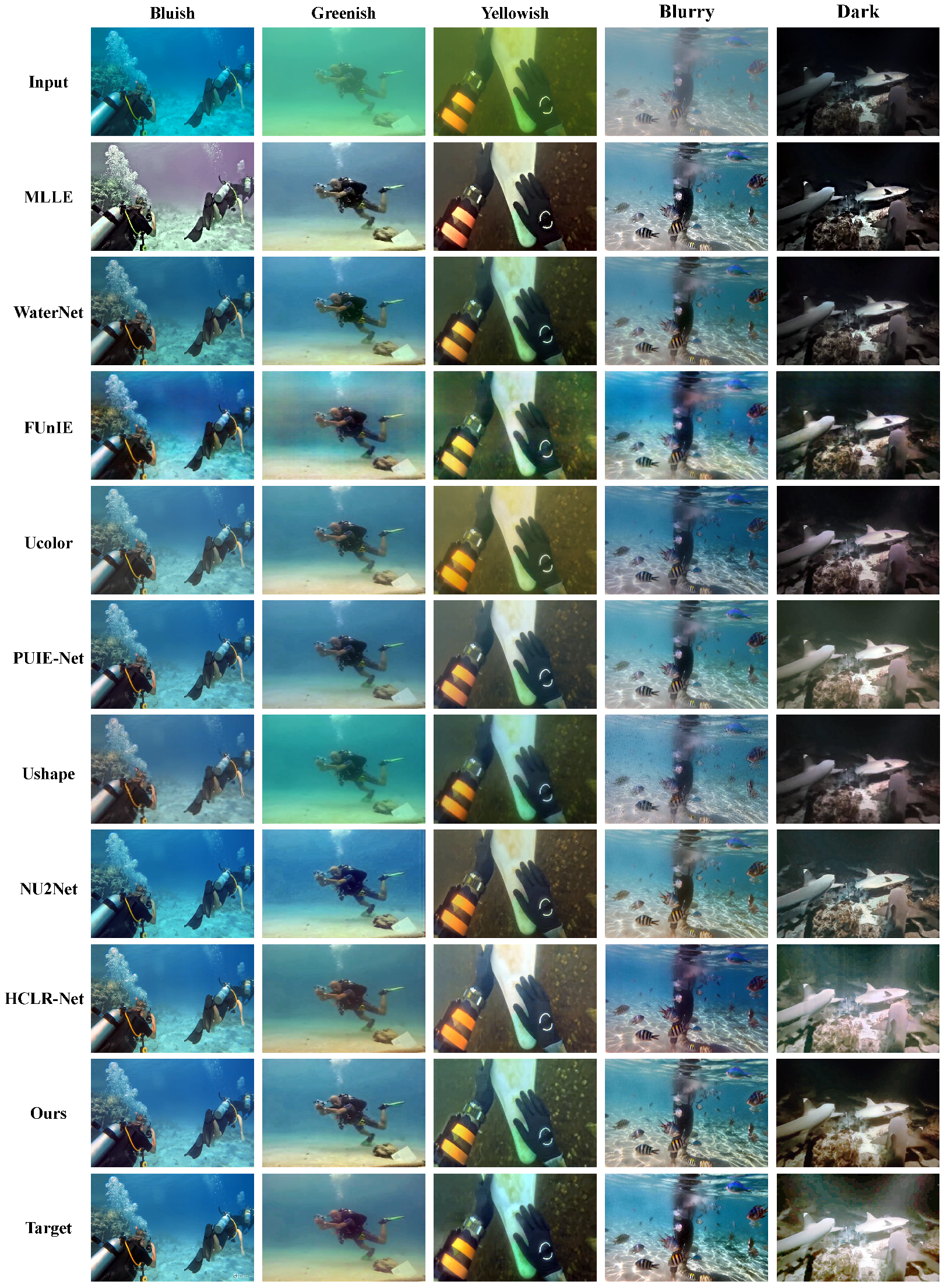
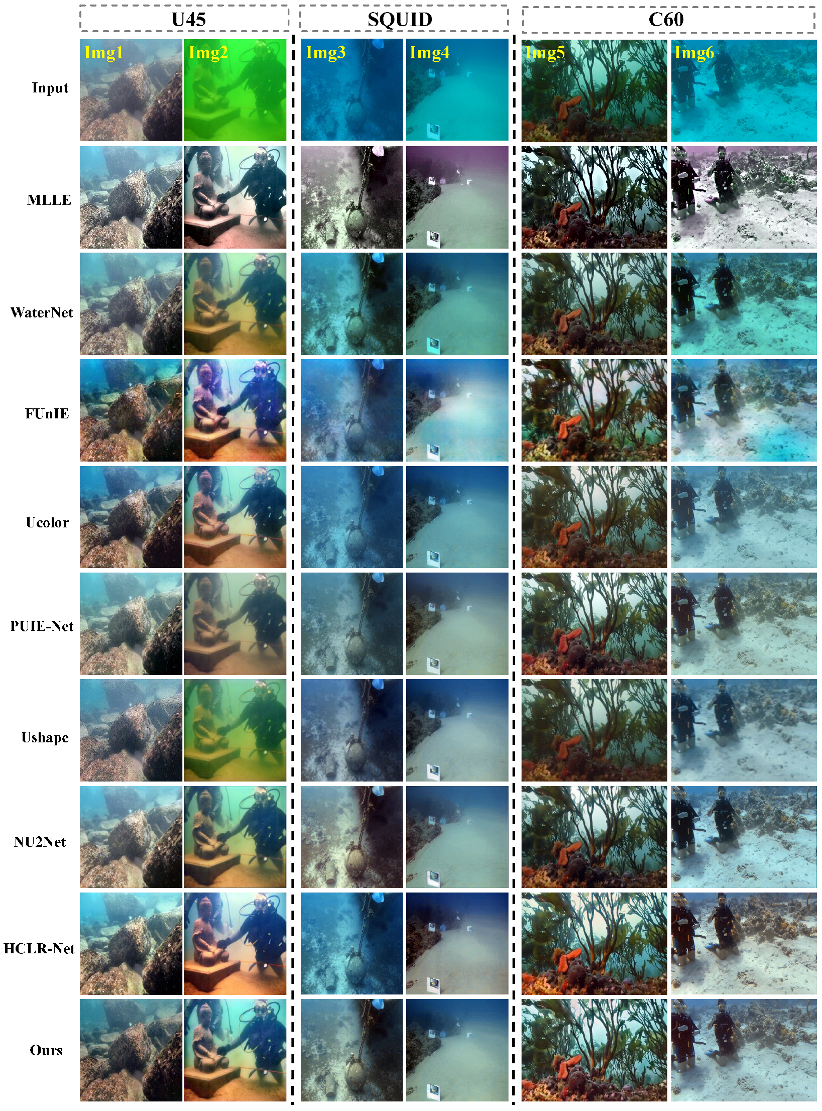
4.4. Visual Comparisons

In this section, the visual effects of different experimental methods on real underwater image datasets are compared. Firstly, we test on the reference dataset U90 by selecting images of underwater scenes with five different distortion types. As illustrated in Figure 7, the images from left to right display color distortions such as bluish, greenish, and yellowish, as well as blurriness and being darker. It can be observed that the MLLE method performs poorly when handling underwater images with bluish distortion, resulting in significant color discrepancies in the enhanced results. Both the WaterNet and Ucolor methods produce enhanced images that are generally darker, while FUnIE introduces artifacts and local color inconsistencies when processing images with a greenish distortion. Although the PUIE-Net and NU2Net methods generally produce good visual results, PUIE-Net often produces enhanced images with fogging artifacts, while NU2Net occasionally results in images with a bluish tint. In comparison, our method effectively handles various types of distortions, delivering enhanced images with superior brightness and contrast, and achieving closer alignment with the reference images.

Subsequently, we compared the visual performance of different methods on the U45, SQUID, and C60 test sets, as illustrated in Figure 8. These datasets are characterized by more pronounced color distortion and low contrast, which often pose significant challenges for conventional methods. We selected representative images from three datasets exhibiting severe bluish, severe greenish, and issues such as blurriness and dimness. It is observed that methods such as MLLE, WaterNet, FUnIE, and Ucolor do not effectively handle all these diverse scenarios simultaneously. For instance, MLLE often introduces additional color distortions, resulting in a purple tint in the images. While FUnIE performs well in improving blurry images, it exhibits localized color artifacts in images with blue distortions. The latest NU2Net method also shows suboptimal performance on blurry and dark images. Clearly, when image distortions are severe, these methods struggle to simultaneously address color distortions, structural distortions, and detail blurring. In contrast, our method consistently demonstrates superior visual quality across all three datasets, with improved image contrast, saturation, and color fidelity. The visualization results across different test sets further indicate that our method exhibits strong robustness and generalization capabilities.

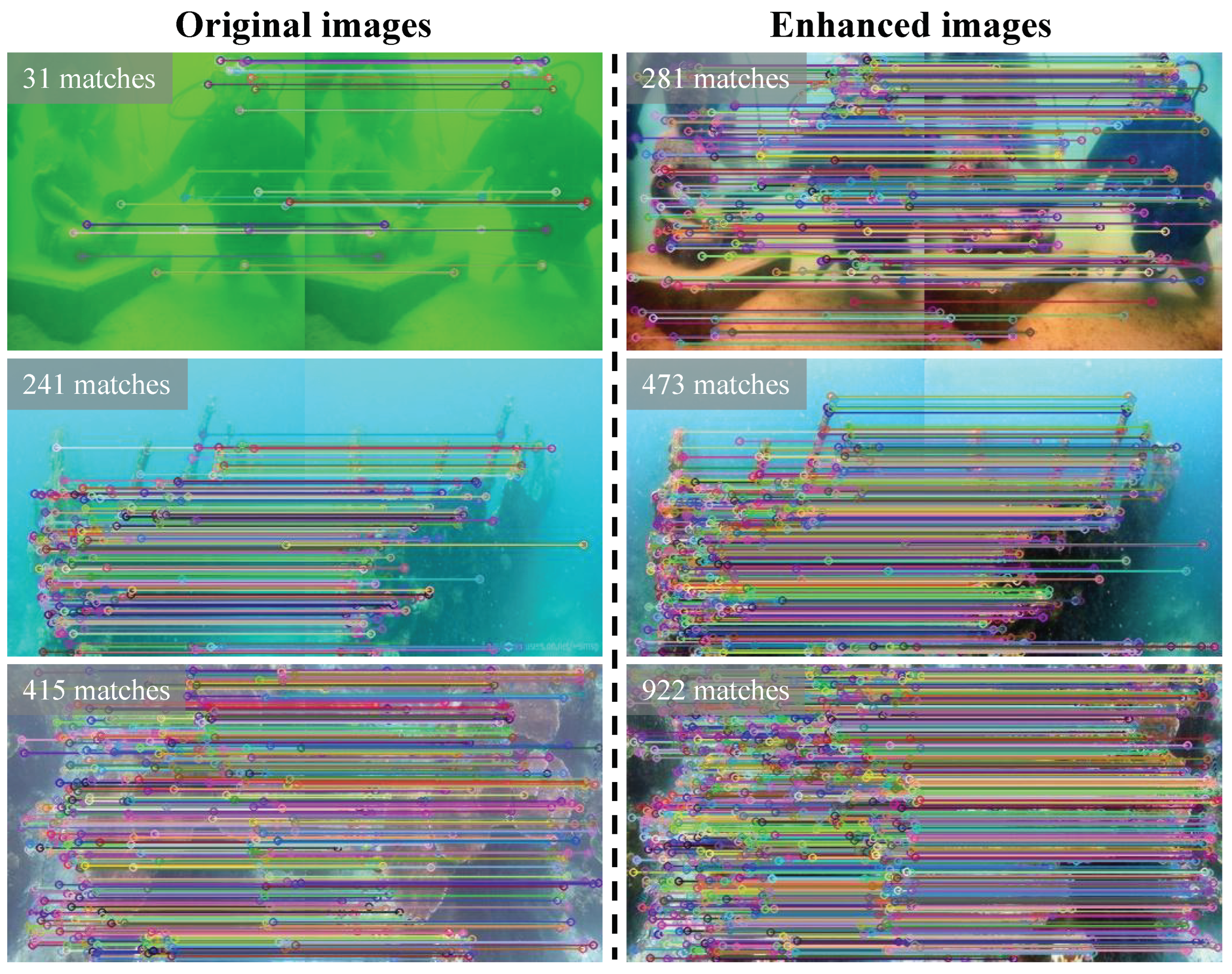
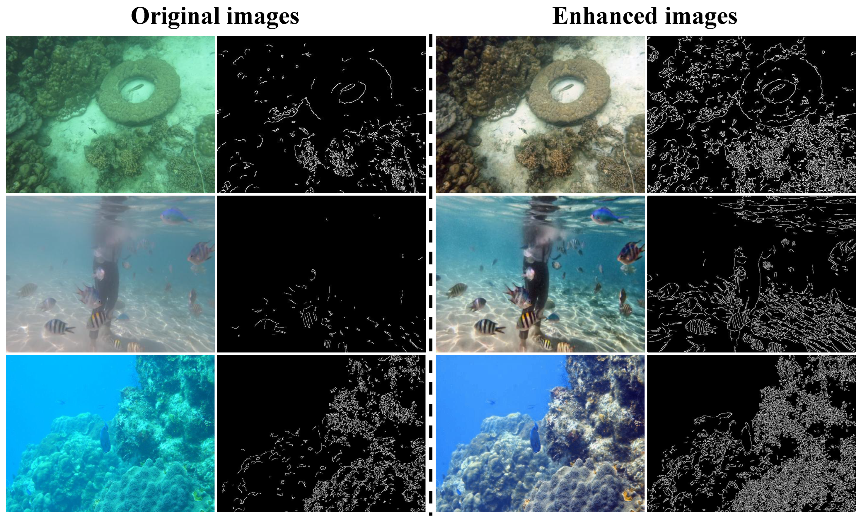
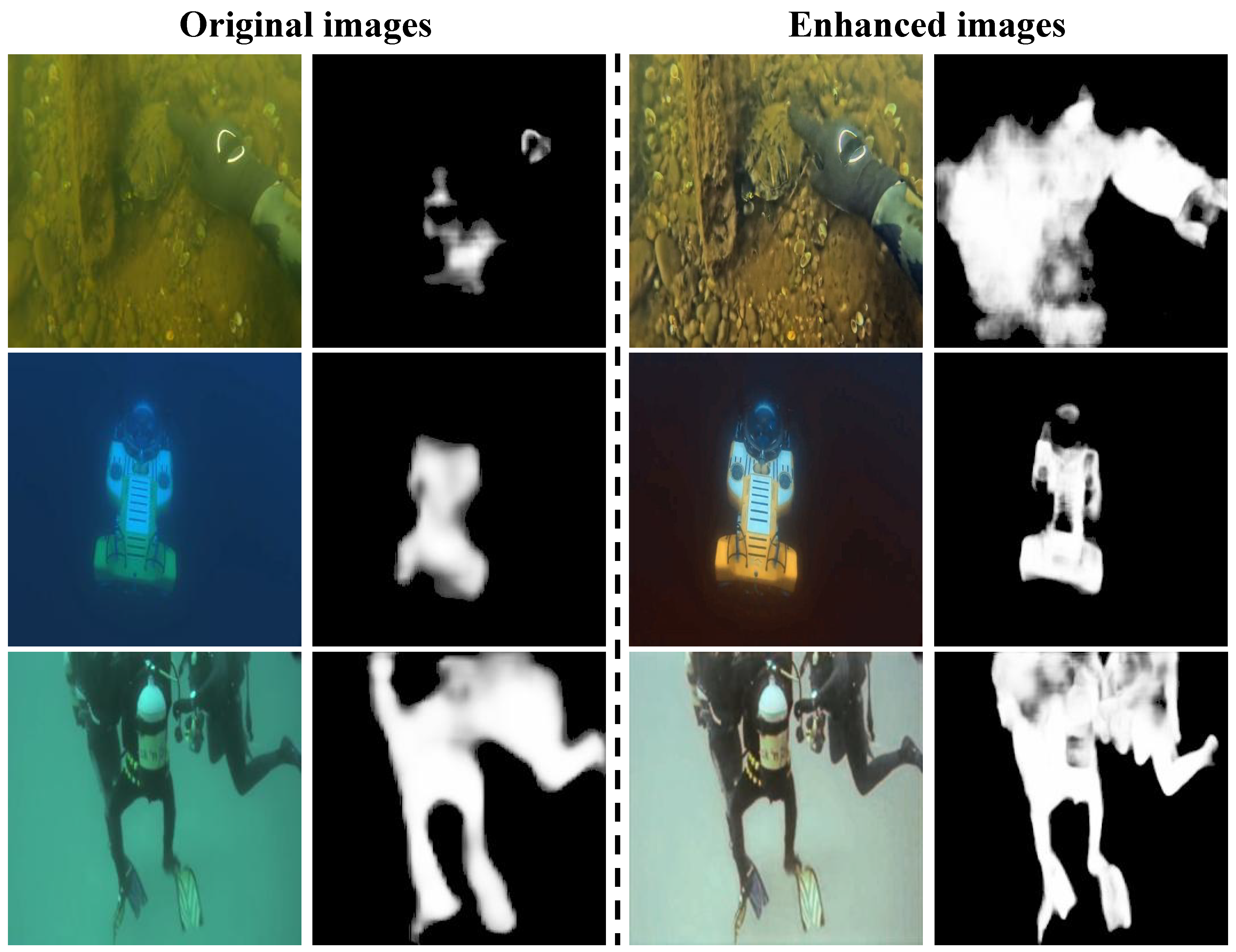
4.5. Application Test

To assess the effectiveness of our method in downstream tasks, we applied the enhanced images to various underwater applications, including feature matching, edge detection, and saliency object detection. The results of feature matching using the Scale-Invariant Feature Transform (SIFT) [48] algorithm are shown in Figure 9. It can be observed that the number of feature matching points in the enhanced images is significantly higher compared to the original images, indicating that our method effectively restores keypoint information. Figure 10 displays the outcomes of edge detection using the Canny edge detector [49]. The enhanced images reveal more complete edge contours, demonstrating that our method effectively recovers edges in underwater images. Figure 11 presents the results of saliency detection using the SVAM model [50]. The saliency maps from the enhanced images show clearer object information, suggesting that our method improves the performance of saliency object detection. The results indicate that our proposed method significantly improves the performance of downstream tasks by enhancing the quality of underwater images, demonstrating its importance in various underwater applications.

4.6. Ablation Study

4.6.1. Impact of Different Modules on Experimental Results

In order to validate the effectiveness of our proposed individual modules, we performed ablation experiments on the U90 dataset, and the experimental results are shown in

Table 3. Impact of different modules on experimental results.↑ indicates that a higher value is better.

Vanilla Conv	DEConv	Fine-tune	PSNR ↑	SSIM ↑
✔			23.113	0.931
	✔		23.287	0.930
	✔	✔	23.436	0.935

. It can be observed that the introduction of difference convolution significantly enhances the model’s performance. To illustrate its superiority more intuitively, we conducted a visualization comparing with and without difference convolution, as shown in Figure 4. The introduction of the difference convolution module enables the model to more effectively extract texture features from images. Next, to further validate the effectiveness of the proposed unsupervised loss fine-tuning module, we conducted ablation experiments with and without the Gaussian degradation-based URanker loss module. It can be seen that after incorporating the Gaussian degradation-based URanker loss module for fine-tuning, the model’s PSNR metric improved by 0.15 dB. The above experimental results effectively verify the superiority of our proposed individual modules. In order to verify the usefulness of each module more visually, we have also visualized the enhancement results using different modules. As shown in Figure 12, it can be noticed that the best visualization is obtained when using difference convolution and using fine-tuning.

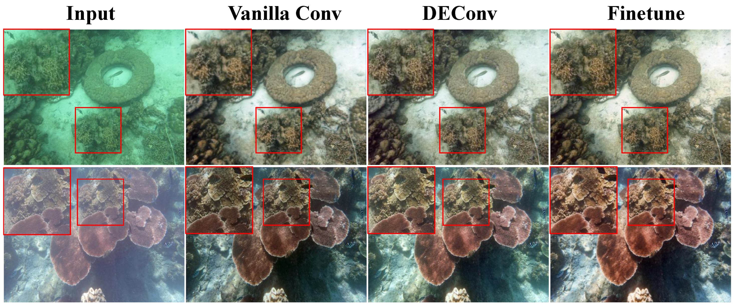
4.6.2. Impact of Different Convolutions on Experimental Results

To assess the importance of difference convolution, we conducted a comparative experiment on the U90 test set to evaluate the impact of various convolution types on the performance of the enhancement network. Specifically, we compared standard convolution (Conv), the combination of standard and dilated convolution (Conv + Dilated), the combination of standard and deformable convolution (Conv + Deformable), and the combination of standard and difference convolution (Conv + Diff). The results, as shown in

Table 4. Impact of different convolutions on experimental results. ↑ indicates that a higher value is better.

Convolution	PSNR ↑	SSIM ↑
Conv	23.113	0.931
Conv + Dilated	22.976	0.921
Conv + Deformable	23.151	0.925
Conv + Diff (ours)	23.287	0.930

, reveal that, compared to the baseline model using only standard convolution, incorporating dilated convolution led to a decrease in performance. This is likely due to the expanded receptive field in dilated convolution, which captures broader global information, but excessive expansion may result in the loss of local details, thus impairing the model’s ability to recover fine-grained image features and textures. While deformable convolution, which learns dynamic offsets for the convolution kernels, improves model performance by flexibly capturing deformed features, the additional parameters and computational cost may have negatively affected training efficiency. In contrast, the combination with difference convolution yielded the best performance. This is likely because difference convolution is more effective at extracting texture features, resulting in more precise image restoration.

5. Conclusions

In this paper, we introduce a UIE network based on difference convolution and propose a Gaussian degradation-based URanker loss module for the fine-tuning phase. Difference convolution enables the model to effectively capture image gradient information and improve the model feature extraction capability. Additionally, to more effectively integrate features from the encoder and decoder, we employed a spatial attention-based fusion module. A normalization module is also used at the final stage of the model, which effectively enhances its performance. During the fine-tuning phase, the incorporation of the Gaussian degradation-based URanker loss module mitigates the challenge of insufficient labels in underwater image datasets. By leveraging the URanker score differences between images enhanced before and after degradation, this module effectively constrains the model’s convergence direction and enhances its generalization ability. Extensive experiments validate the superiority and broad applicability of our proposed UIE method, and various application tests further confirm its effectiveness for underwater downstream tasks.

It can be observed that our model is a deep learning model heavily reliant on the quality of reference images. However, obtaining high-quality reference images has always been a challenge in UIE tasks. Although we have proposed an unsupervised loss module to reduce the model’s dependence on reference images, there are still some limitations, such as the need for effective no-reference-image quality assessment metrics. Developing such metrics for underwater images remains a challenging task. We hope that our next research project will reduce the model’s dependence on high-quality reference images and leverage more effective prior knowledge to decrease the number of model parameters.

References

1. Paull, L.; Saeedi, S.; Seto, M.; Li, H. AUV Navigation and Localization: A Review. IEEE J. Ocean. Eng. 2013, 39, 131–149. [Google Scholar] [CrossRef]
2. Cong, R.; Zhang, Y.; Fang, L.; Li, J.; Zhao, Y.; Kwong, S. RRNet: Relational Reasoning Network With Parallel Multiscale Attention for Salient Object Detection in Optical Remote Sensing Images. IEEE Trans. Geosci. Remote Sens. 2021, 60, 5613311. [Google Scholar] [CrossRef]
3. Schettini, R.; Corchs, S. Underwater Image Processing: State of the Art of Restoration and Image Enhancement Methods. EURASIP J. Adv. Signal Process. 2010, 2010, 746052. [Google Scholar] [CrossRef]
4. Ancuti, C.; Ancuti, C.O.; Haber, T.; Bekaert, P. Enhancing Underwater Images and Videos by Fusion. In Proceedings of the 2012 IEEE Conference on Computer Vision and Pattern Recognition, Providence, RI, USA, 16–21 June 2012; pp. 81–88. [Google Scholar]
5. Iqbal, K.; Odetayo, M.; James, A.; Salam, R.A.; Talib, A.Z.H. Enhancing the Low Quality Images Using Unsupervised Colour Correction Method. In Proceedings of the 2010 IEEE International Conference on Systems, Man and Cybernetics, Istanbul, Turkey, 10–13 October 2010; pp. 1703–1709. [Google Scholar]
6. He, K.; Sun, J.; Tang, X. Single Image Haze Removal Using Dark Channel Prior. IEEE Trans. Pattern Anal. Mach. Intell. 2010, 33, 2341–2353. [Google Scholar] [PubMed]
7. Li, C.Y.; Guo, J.C.; Cong, R.M.; Pang, Y.W.; Wang, B. Underwater Image Enhancement by Dehazing with Minimum Information Loss and Histogram Distribution Prior. IEEE Trans. Image Process. 2016, 25, 5664–5677. [Google Scholar] [CrossRef] [PubMed]
8. Li, C.; Guo, C.; Ren, W.; Cong, R.; Hou, J.; Kwong, S.; Tao, D. An Underwater Image Enhancement Benchmark Dataset and Beyond. IEEE Trans. Image Process. 2019, 29, 4376–4389. [Google Scholar] [CrossRef] [PubMed]
9. Li, C.; Anwar, S.; Hou, J.; Cong, R.; Guo, C.; Ren, W. Underwater Image Enhancement via Medium Transmission-Guided Multi-Color Space Embedding. IEEE Trans. Image Process. 2021, 30, 4985–5000. [Google Scholar] [CrossRef] [PubMed]
10. Guo, C.; Wu, R.; Jin, X.; Han, L.; Zhang, W.; Chai, Z.; Li, C. Underwater Ranker: Learn Which is Better and How to be Better. In Proceedings of the AAAI Conference on Artificial Intelligence, Washington, DC, USA, 7–14 February 2023; Volume 37, pp. 702–709. [Google Scholar]
11. Islam, M.J.; Xia, Y.; Sattar, J. Fast Underwater Image Enhancement for Improved Visual Perception. IEEE Robot. Autom. Lett. 2020, 5, 3227–3234. [Google Scholar] [CrossRef]
12. Naik, A.; Swarnakar, A.; Mittal, K. Shallow-UWnet: Compressed Model for Underwater Image Enhancement (Student Abstract). In Proceedings of the AAAI Conference on Artificial Intelligence, Virtual, 2–9 February 2021; Volume 35, pp. 15853–15854. [Google Scholar]
13. Chen, Z.; He, Z.; Lu, Z.M. DEA-Net: Single Image Dehazing Based on Detail-Enhanced Convolution and Content-Guided Attention. IEEE Trans. Image Process. 2024, 33, 1002–1015. [Google Scholar] [CrossRef] [PubMed]
14. Peng, L.; Zhu, C.; Bian, L. U-Shape Transformer for Underwater Image Enhancement. IEEE Trans. Image Process. 2023, 32, 3066–3079. [Google Scholar] [CrossRef] [PubMed]
15. Johnson, J.; Alahi, A.; Fei-Fei, L. Perceptual Losses for Real-Time Style Transfer and Super-Resolution. In Computer Vision—ECCV 2016, Proceedings of the 14th European Conference, Amsterdam, The Netherlands, 11–14 October 2016; Proceedings Part II 14; Springer: Berlin/Heidelberg, Germany, 2016; pp. 694–711. [Google Scholar]
16. Song, Y.; He, Z.; Qian, H.; Du, X. Vision Transformers for Single Image Dehazing. IEEE Trans. Image Process. 2023, 32, 1927–1941. [Google Scholar] [CrossRef] [PubMed]
17. Li, X.; Wang, W.; Hu, X.; Yang, J. Selective Kernel Networks. In Proceedings of the 2019 IEEE/CVF Conference on Computer Vision and Pattern Recognition (CVPR), Long Beach, CA, USA, 15–20 June 2019; pp. 510–519. [Google Scholar] [CrossRef]
18. Drews, P.; Nascimento, E.; Moraes, F.; Botelho, S.; Campos, M. Transmission Estimation in Underwater Single Images. In Proceedings of the IEEE International Conference on Computer Vision Workshops, Sydney, Australia, 2–8 December 2013; pp. 825–830. [Google Scholar]
19. Drews, P.L.; Nascimento, E.R.; Botelho, S.S.; Campos, M.F.M. Underwater Depth Estimation and Image Restoration Based on Single Images. IEEE Comput. Graph. Appl. 2016, 36, 24–35. [Google Scholar] [CrossRef] [PubMed]
20. Awan, H.S.A.; Mahmood, M.T. Underwater Image Restoration through Color Correction and UW-Net. Electronics 2024, 13, 199. [Google Scholar] [CrossRef]
21. Jia, H.; Xiao, Y.; Wang, Q.; Chen, X.; Han, Z.; Tang, Y. Underwater Image Enhancement Network Based on Dual Layers Regression. Electronics 2024, 13, 196. [Google Scholar] [CrossRef]
22. Qian, J.; Li, H.; Zhang, B. HA-Net: A Hybrid Algorithm Model for Underwater Image Color Restoration and Texture Enhancement. Electronics 2024, 13, 2623. [Google Scholar] [CrossRef]
23. Fu, Z.; Wang, W.; Huang, Y.; Ding, X.; Ma, K.K. Uncertainty Inspired Underwater Image Enhancement. In Proceedings of the European Conference on Computer Vision, Tel Aviv, Israel, 23–27 October 2022; pp. 465–482. [Google Scholar]
24. Yan, H.; Zhang, Z.; Xu, J.; Wang, T.; An, P.; Wang, A.; Duan, Y. UW-CycleGAN: Model-Driven CycleGAN for Underwater Image Restoration. IEEE Trans. Geosci. Remote Sens. 2023, 61, 4207517. [Google Scholar] [CrossRef]
25. Chang, S.; Gao, F.; Zhang, Q. Underwater Image Enhancement Method Based on Improved GAN and Physical Model. Electronics 2023, 12, 2882. [Google Scholar] [CrossRef]
26. Zhou, J.; Sun, J.; Li, C.; Jiang, Q.; Zhou, M.; Lam, K.M.; Zhang, W.; Fu, X. HCLR-Net: Hybrid Contrastive Learning Regularization with Locally Randomized Perturbation for Underwater Image Enhancement. Int. J. Comput. Vis. 2024, 132, 4132–4156. [Google Scholar] [CrossRef]
27. Cong, R.; Yang, W.; Zhang, W.; Li, C.; Guo, C.L.; Huang, Q.; Kwong, S. PUGAN: Physical Model-Guided Underwater Image Enhancement Using GAN With Dual-Discriminators. IEEE Trans. Image Process. 2023, 32, 4472–4485. [Google Scholar] [CrossRef]
28. Ojala, T.; Pietikainen, M.; Maenpaa, T. Multiresolution Gray-Scale And Rotation Invariant Texture Classification with Local Binary Patterns. IEEE Trans. Pattern Anal. Mach. Intell. 2002, 24, 971–987. [Google Scholar] [CrossRef]
29. Juefei-Xu, F.; Boddeti, V.N.; Savvides, M. Local Binary Convolutional Neural Networks. In Proceedings of the 2017 IEEE Conference on Computer Vision and Pattern Recognition (CVPR), Honolulu, HI, USA, 21–26 July 2017; pp. 4284–4293. [Google Scholar] [CrossRef]
30. Yu, Z.; Zhao, C.; Wang, Z.; Qin, Y.; Su, Z.; Li, X.; Zhou, F.; Zhao, G. Searching Central Difference Convolutional Networks for Face Anti-spoofing. In Proceedings of the IEEE/CVF Conference on Computer Vision and Pattern Recognition, Seattle, WA, USA, 14–19 June 2020; pp. 5295–5305. [Google Scholar]
31. Yu, Z.; Qin, Y.; Zhao, H.; Li, X.; Zhao, G. Dual-Cross Central Difference Network for Face Anti-Spoofing. In Proceedings of the IJCAI International Joint Conference on Artificial Intelligence, Montreal, BC, Canada, 19–27 August 2021. [Google Scholar]
32. Su, Z.; Liu, W.; Yu, Z.; Hu, D.; Liao, Q.; Tian, Q.; Pietikäinen, M.; Liu, L. Pixel Difference Networks for Efficient Edge Detection. In Proceedings of the IEEE/CVF International Conference on Computer Vision, Montreal, BC, Canada, 11–17 October 2021; pp. 5117–5127. [Google Scholar]
33. Wang, Y.; Guo, J.; Gao, H.; Yue, H. UIEC^ 2-Net: CNN-based Underwater Image Enhancement Using Two Color Space. Signal Process. Image Commun. 2021, 96, 116250. [Google Scholar] [CrossRef]
34. Wang, C.; Shen, H.Z.; Fan, F.; Shao, M.W.; Yang, C.S.; Luo, J.C.; Deng, L.J. EAA-Net: A novel edge assisted attention network for single image dehazing. Knowl.-Based Syst. 2021, 228, 107279. [Google Scholar] [CrossRef]
35. Zhang, H.; Patel, V.M. Densely Connected Pyramid Dehazing Network. In Proceedings of the 2018 IEEE/CVF Conference on Computer Vision and Pattern Recognition, Salt Lake City, UT, USA, 18–22 June 2018; pp. 3194–3203. [Google Scholar] [CrossRef]
36. Sobel, I.; Feldman, G. A 3 × 3 isotropic gradient operator for image processing. Pattern Classif. Scene Anal. 1973, 1968, 271–272. [Google Scholar]
37. Scharr, H. Optimal Operators in Digital Image Processing. Ph.D. Thesis, University of Heidelberg, Heidelberg, Germany, 2000. [Google Scholar]
38. Hu, J.; Shen, L.; Sun, G. Squeeze-and-Excitation Networks. In Proceedings of the IEEE Conference on Computer Vision and Pattern Recognition, Salt Lake City, UT, USA, 18–22 June 2018; pp. 7132–7141. [Google Scholar]
39. Woo, S.; Park, J.; Lee, J.Y.; Kweon, I.S. CBAM: Convolutional Block Attention Module. In Proceedings of the European Conference on Computer Vision (ECCV), Munich, Germany, 8–14 September 2018; pp. 3–19. [Google Scholar]
40. Wu, H.; Qu, Y.; Lin, S.; Zhou, J.; Qiao, R.; Zhang, Z.; Xie, Y.; Ma, L. Contrastive Learning for Compact Single Image Dehazing. In Proceedings of the IEEE/CVF Conference on Computer Vision and Pattern Recognition, Nashville, TN, USA, 19–25 June 2021; pp. 10551–10560. [Google Scholar]
41. Li, H.; Li, J.; Wang, W. A Fusion Adversarial Underwater Image Enhancement Network with a Public Test Dataset. arXiv 2019, arXiv:1906.06819. [Google Scholar]
42. Akkaynak, D.; Treibitz, T. Sea-thru: A Method for Removing Water from Underwater Images. In Proceedings of the IEEE/CVF Conference on Computer Vision and Pattern Recognition, Long Beach, CA, USA, 16–20 June 2019; pp. 1682–1691. [Google Scholar]
43. Zhang, R.; Isola, P.; Efros, A.A.; Shechtman, E.; Wang, O. The Unreasonable Effectiveness of Deep Features as a Perceptual Metric. In Proceedings of the IEEE Conference on Computer Vision and Pattern Recognition, Salt Lake City, UT, USA, 18–22 June 2018; pp. 586–595. [Google Scholar]
44. Panetta, K.; Gao, C.; Agaian, S. Human-Visual-System-Inspired Underwater Image Quality Measures. IEEE J. Ocean. Eng. 2015, 41, 541–551. [Google Scholar] [CrossRef]
45. Yang, M.; Sowmya, A. An Underwater Color Image Quality Evaluation Metric. IEEE Trans. Image Process. 2015, 24, 6062–6071. [Google Scholar] [CrossRef] [PubMed]
46. Peng, Y.T.; Cosman, P.C. Underwater Image Restoration Based on Image Blurriness and Light Absorption. IEEE Trans. Image Process. 2017, 26, 1579–1594. [Google Scholar] [CrossRef] [PubMed]
47. Zhang, W.; Zhuang, P.; Sun, H.H.; Li, G.; Kwong, S.; Li, C. Underwater Image Enhancement Via Minimal Color Loss and Locally Adaptive Contrast Enhancement. IEEE Trans. Image Process. 2022, 31, 3997–4010. [Google Scholar] [CrossRef] [PubMed]
48. Lowe, D.G. Distinctive Image Features from Scale-Invariant Keypoints. Int. J. Comput. Vis. 2004, 60, 91–110. [Google Scholar] [CrossRef]
49. Canny, J. A Computational Approach to Edge Detection. IEEE Trans. Pattern Anal. Mach. Intell. 1986, PAMI-8, 679–698. [Google Scholar] [CrossRef]
50. Islam, M.J.; Wang, R.; Sattar, J. SVAM: Saliency-guided Visual Attention Modeling by Autonomous Underwater Robots. arXiv 2020, arXiv:2011.06252. [Google Scholar]
Figure 1. Example of the color distribution of underwater raw images and their corresponding enhanced images: the left side represents the raw images and their tricolor histograms, while the right side represents the enhanced images and their tricolor histograms.
Electronics 13 05003 g001
Figure 2. The proposed framework of UIE network. In the upper part, the left side illustrates the model’s training and inference stages, while the right side represents the model’s fine-tuning phase. The lower half details the specific composition of the network modules.
Electronics 13 05003 g002
Figure 3. The derivation of Vertical Difference Convolution (VDC).
Electronics 13 05003 g003
Figure 4. Visualization of intermediate features of the model. w/o DeConv represents not using difference convolutions, while w/ DeConv represents the use of difference convolutions.
Electronics 13 05003 g004
Figure 5. Visualization of feature maps at different decoder stages. Levels 1 to 3 represent successive decoder stages, with feature maps increasing in size sequentially.
Electronics 13 05003 g005
Figure 6. UCIQE and UIQM values for each image in the non-reference test set across different methods.
Electronics 13 05003 g006
Figure 7. Visual comparison of enhancement results for the U90 test set. From top to bottom, the original underwater image, MLLE [47], WaterNet [8], FUnIE [11], Ucolor [9], U-shape [14], NU2Net [10], HCLR-Net [26], our method, and the reference image.
Electronics 13 05003 g007
Figure 8. Visual comparison of enhancement results for the U45, SQUID, and C60 test sets. From top to bottom, the original underwater image, MLLE [47], WaterNet [8], FUnIE [11], Ucolor [9], U-shape [14], NU2Net [10], HCLR-Net [26], and our method.
Electronics 13 05003 g008
Figure 9. The SIFT keypoint matching test: degraded (left) and our enhanced images (right).
Electronics 13 05003 g009
Figure 10. The Canny edge detection test: degraded (left) and our enhanced images (right).
Electronics 13 05003 g010
Figure 11. The SVAM saliency detection test: degraded (left) and our enhanced images (right).
Electronics 13 05003 g011
Figure 12. Ablation study of the performance of the model components.
Electronics 13 05003 g012