
Research on UAV Autonomous Recognition and Approach Method for Linear Target Splicing Sleeves Based on Deep Learning and Active Stereo Vision


Abstract
1. Introduction
- (1)
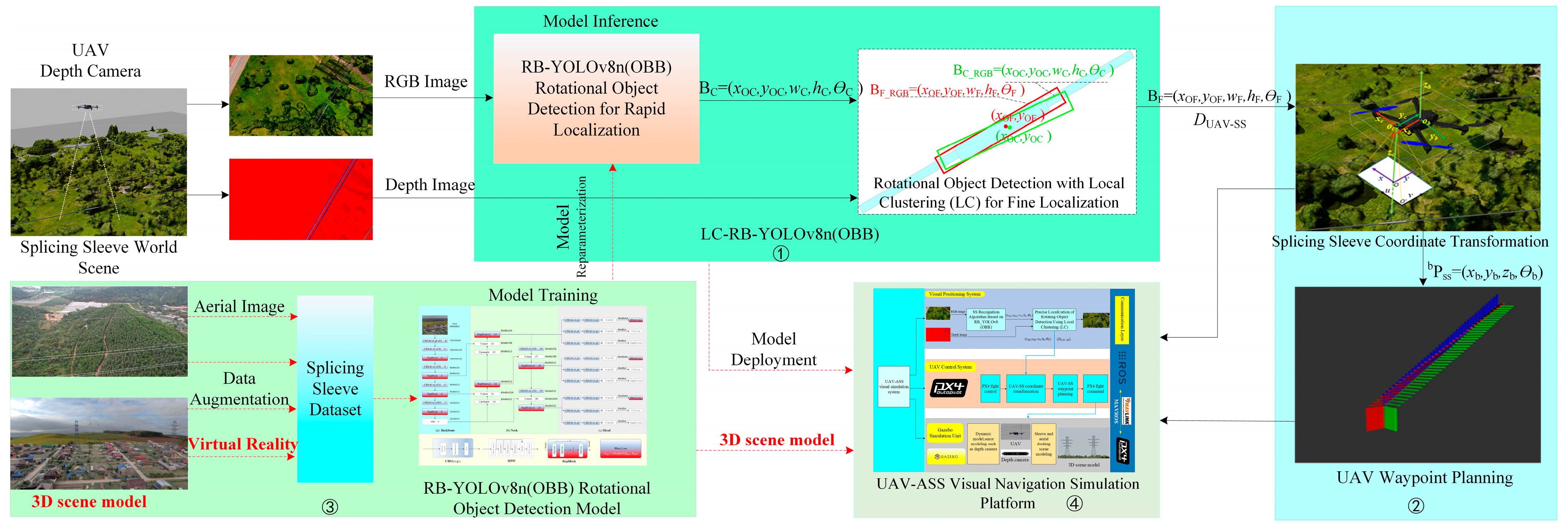
- A two-stage rapid and precise localization strategy based on the LC-RB-YOLOv8n (OBB) framework is proposed to address the issues of inaccurate positioning and unstable distance measurement faced by UAVs during high-altitude search, recognition, and approach tasks involving linear target splicing sleeves. This strategy first utilizes reparameterization of training results to obtain a lightweight and fast splicing sleeve recognition model. Subsequently, a local clustering algorithm is employed to enhance the positioning accuracy of splicing sleeves, and finally, the depth values of the splicing sleeves are extracted using the linear nearest neighbor averaging method.
- (2)
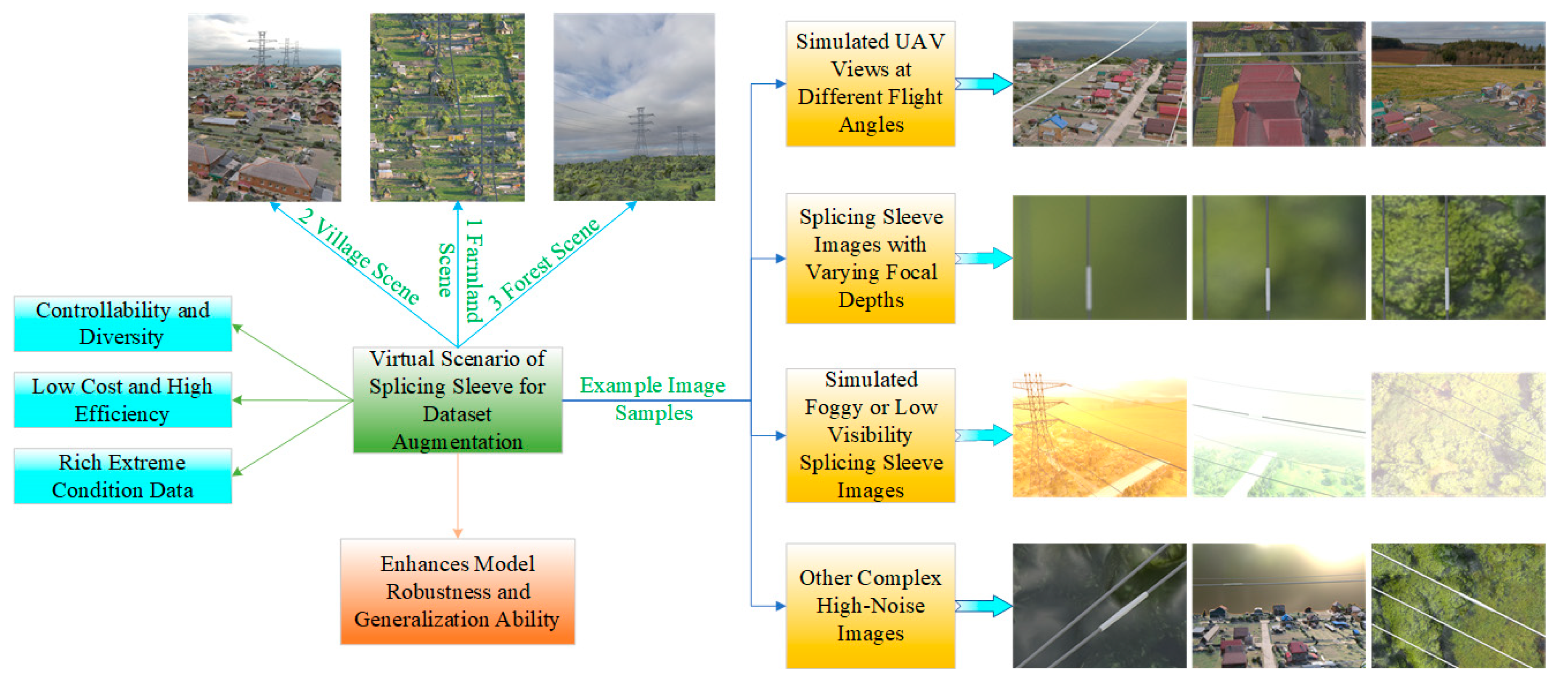
- To address the high costs and safety risks associated with image acquisition of splicing sleeves on high-altitude power transmission lines, as well as the difficulties in obtaining sufficient and representative data under complex and variable weather conditions and terrain in real scenarios, the construction of realistic splicing sleeve virtual scenes is proposed. This approach expands the real splicing sleeve dataset Dreal to meet the requirements of diverse scenarios, thereby enhancing the robustness and generalization ability of the splicing sleeve recognition model.
- (3)
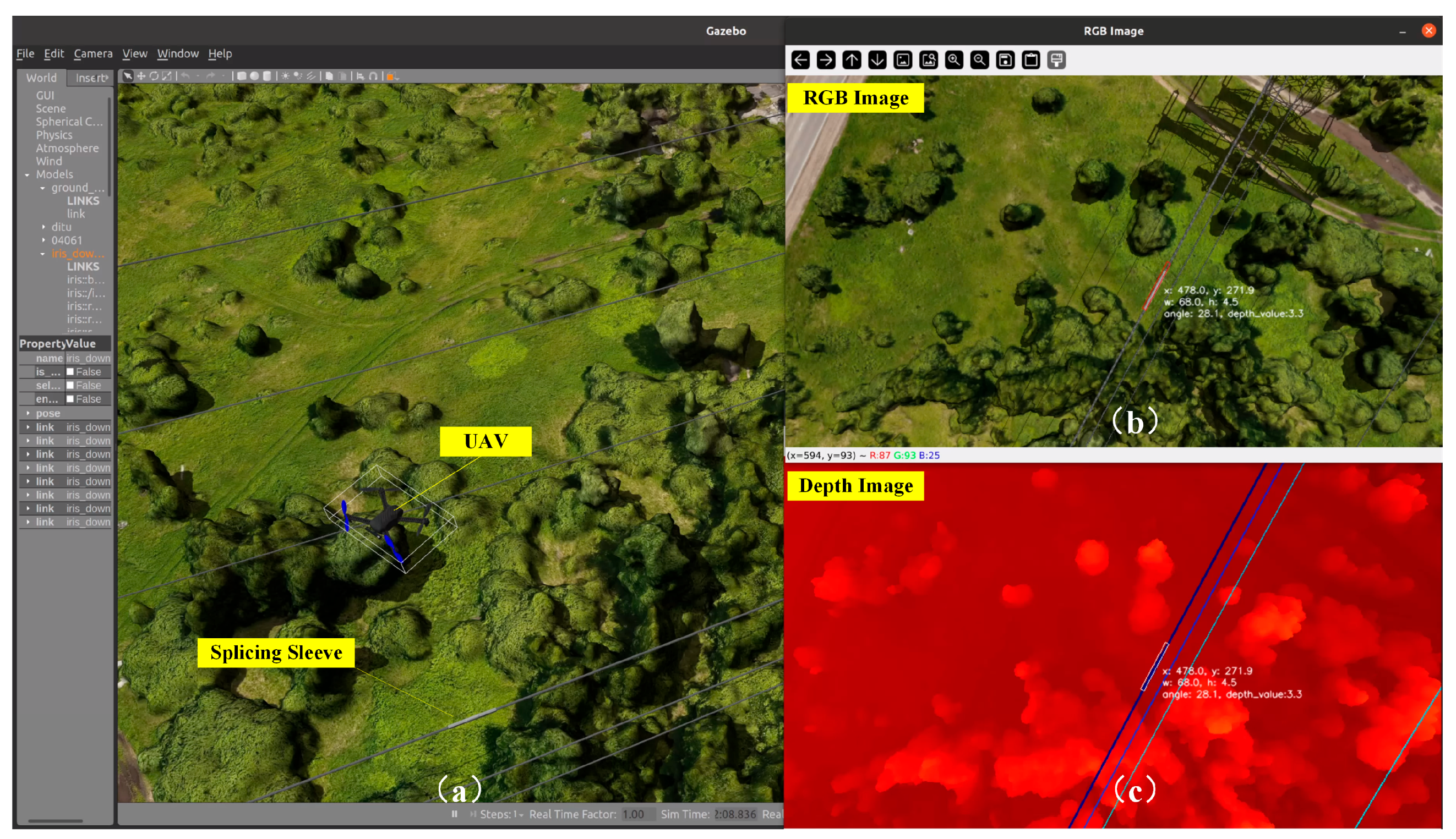
- To reduce the high-risk nature of visual navigation experiments involving UAV recognition and approach to high-altitude splicing sleeves and to improve algorithm verification and testing efficiency, a UAV-ASS visual simulation platform is proposed. This platform is built using the PX4 open-source UAV flight control system, the ROS, and the physical simulation platform GAZEBO, effectively reducing testing costs and safety risks.
2. Related Work
2.1. UAV Stereo Vision for Key Target Recognition and Localization
2.2. UAV Autonomous Docking and Landing Technology
2.3. Uniqueness of This Study
3. Methodology
3.1. A Two-Stage Rapid and Accurate Localization Strategy for Rotational Targets (LC-RB-YOLOv8n(OBB))
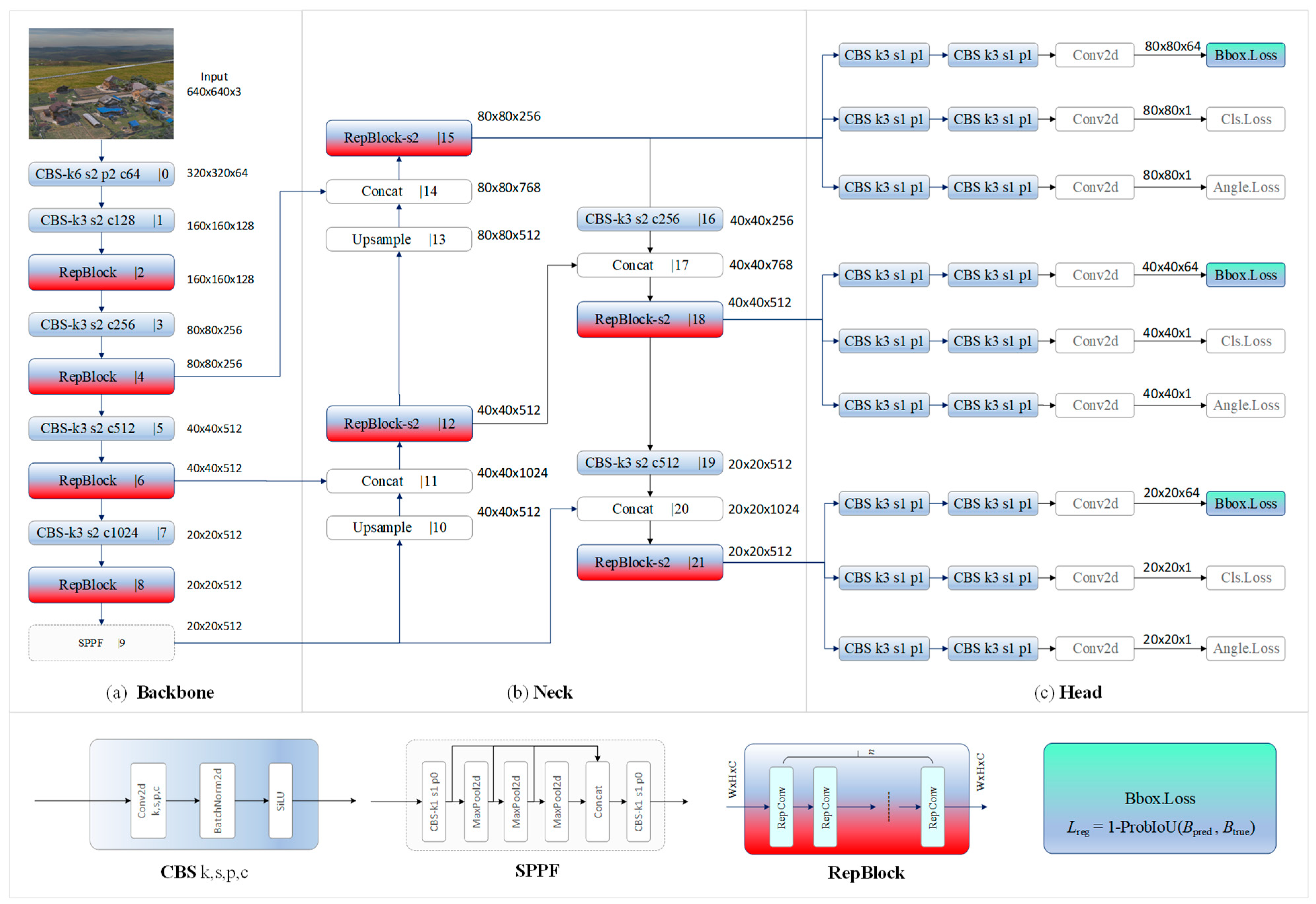
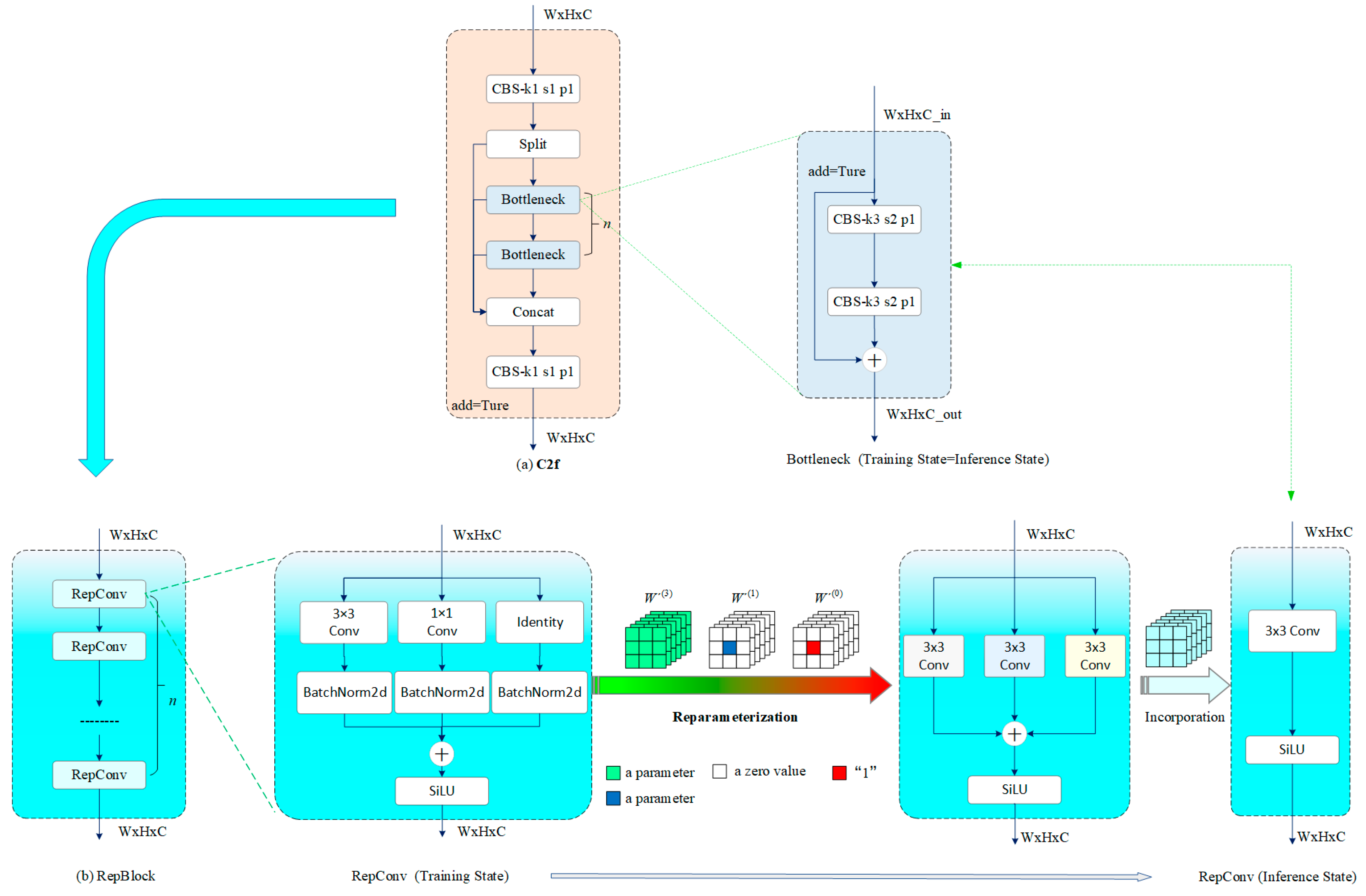
3.1.1. Rapid Localization of Rotational Object Detection Using RB-YOLOv8n(OBB)
- (1)
- In the Conveq calculation for the 3 × 3 conv branch, since the weight W(3) obtained during training has the same dimensions as the weight in the inference phase, the equivalent weight W′(3) and bias b′(3) for the 3 × 3 conv can be directly calculated by substituting the trained values of W(3), μ(3), σ2(3), γ(3), β(3) and ε(3) into Equation (2).
- (2)
- In the Conveq for the 1 × 1 conv branch, since the weight W(1) obtained during training does not have the same dimensions as the weight in the inference phase, it can be expanded using a padding operation (Pad) to form W(1)3×3, ensuring that W(1)3×3 matches the dimensions of the weight in the inference phase. The expanded W(1)3×3 is denoted as:
- (3)
- In the Conveq calculation for the Identity branch, since this branch only contains the BN layer, a 3 × 3 pseudo convolutional kernel is first created, with the center of the kernel set to 1 and the remaining elements set to zero. The number of convolutional kernels is made equal to the number of input channels. The pseudo weight for this branch, W(0), is denoted as:
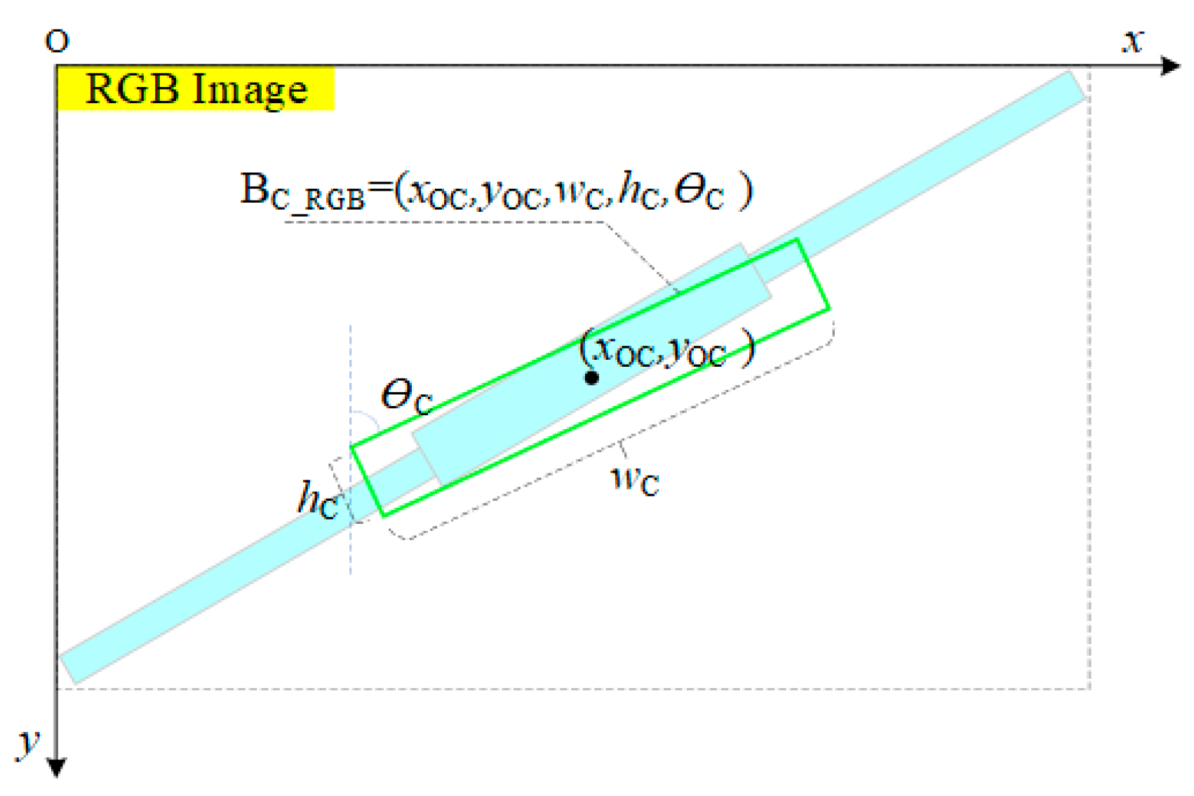
3.1.2. Fine Localization of Rotational Object Detection Using Local Clustering (LC)
- (1)
- Determination of the Local Region boundary RDE for the Rapidly Localized Rectangular Box of the Splicing Sleeve:
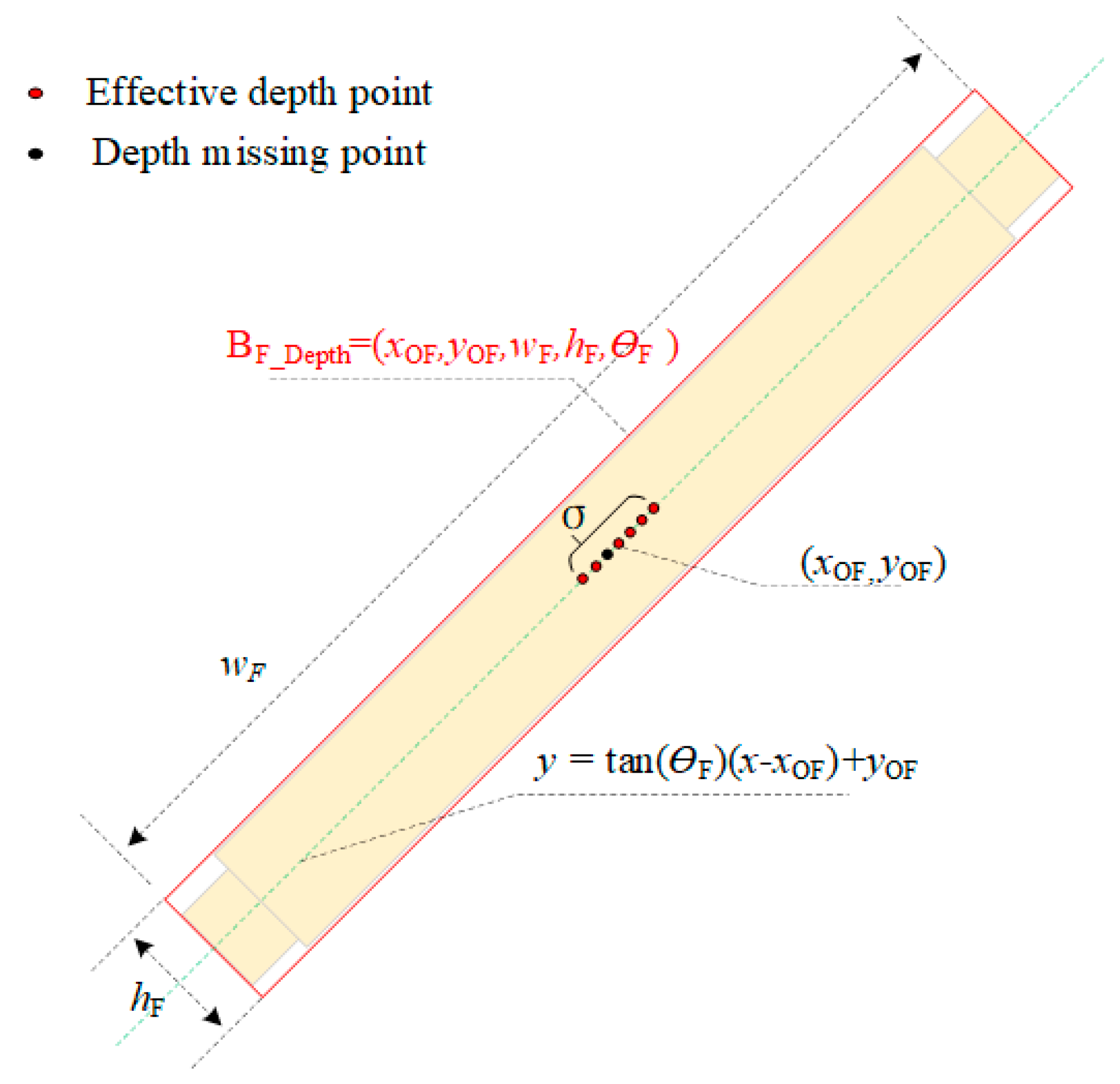
- (2)
- Clustering and Fitting of Depth Values DR in the Local Region RDE
- ①
- Clustering of Depth Values DR in RDE
- ②
- Depth Value DR Clustering and Fitting
| Algorithm 1 Fusion K-Means clustering rotating target fine-tuning algorithm | |
| Input:depth_image, rgb_image Output:rect_new(Fine-tuning rotating target recognition results), depth_value | |
| 1. | k_means_trimming_functions(rag_image, depth_image) |
| 2. | result = inference_detector(model, rgb_image); // Rotating target recognition results |
| 3. | key_point = extract_clustering_target_regions(result); // Return the key parameters of the horizontal box area of the rotating target result according to the result. |
| 4. | if key_point! = 0: // Determine whether there are recognition results that satisfy the conditions |
| 5. | depth_target_regions = depth_image(key_point); // Cut horizontal box area on depth_image |
| 6. | num_clusters = 3; // Set the initial clustering value. When shooting from high altitude, determine the clustering value based on the complexity of the background. |
| 7. | cluster_depth_image = K_Means_fuction(num_clusters,depth_target_regions); // Return clustering results |
| 8. | min_depth_class = np.argmin([np.mean(depth_target_regions[cluster_depth_image == i]) for i in range(num_clusters)]); // Finding the Depth Minimum Category |
| 9. | rect = cv2.minAreaRect(points_cv); // Fitting a minimum area rotating frame |
| 10. | center_x, center_y, width, heigth, angle = rect; // Get the center point coordinates, width, height and rotation angle of the rotated box after fine-tuning. |
| 11. | depth_value = depth_target_regions[int(center_y), int(center_x)]; // Extract the depth value of the center point of the rotating frame |
| 12. | rect_new = rect + key_points; // Adjust the spinning frame coordinates to depth_image coordinates |
| 13. | return (rect_new, depth_value); // Returns the coordinates and depth of the original rotated frame. |
| 14. | else: |
| 15. | return (0,0); // Returns the null value |
3.2. UAV-ASS Coordinate Transformation and Waypoint Planning
4. Experimental and Results Analysis
4.1. UAV Recognition and Localization Experiments for Splicing Sleeves on Overhead Transmission Lines
4.1.1. Construction of the Experimental Dataset DSS
4.1.2. RB-YOLOv8n(OBB) Rotational Object Detection Rapid Localization Experiment
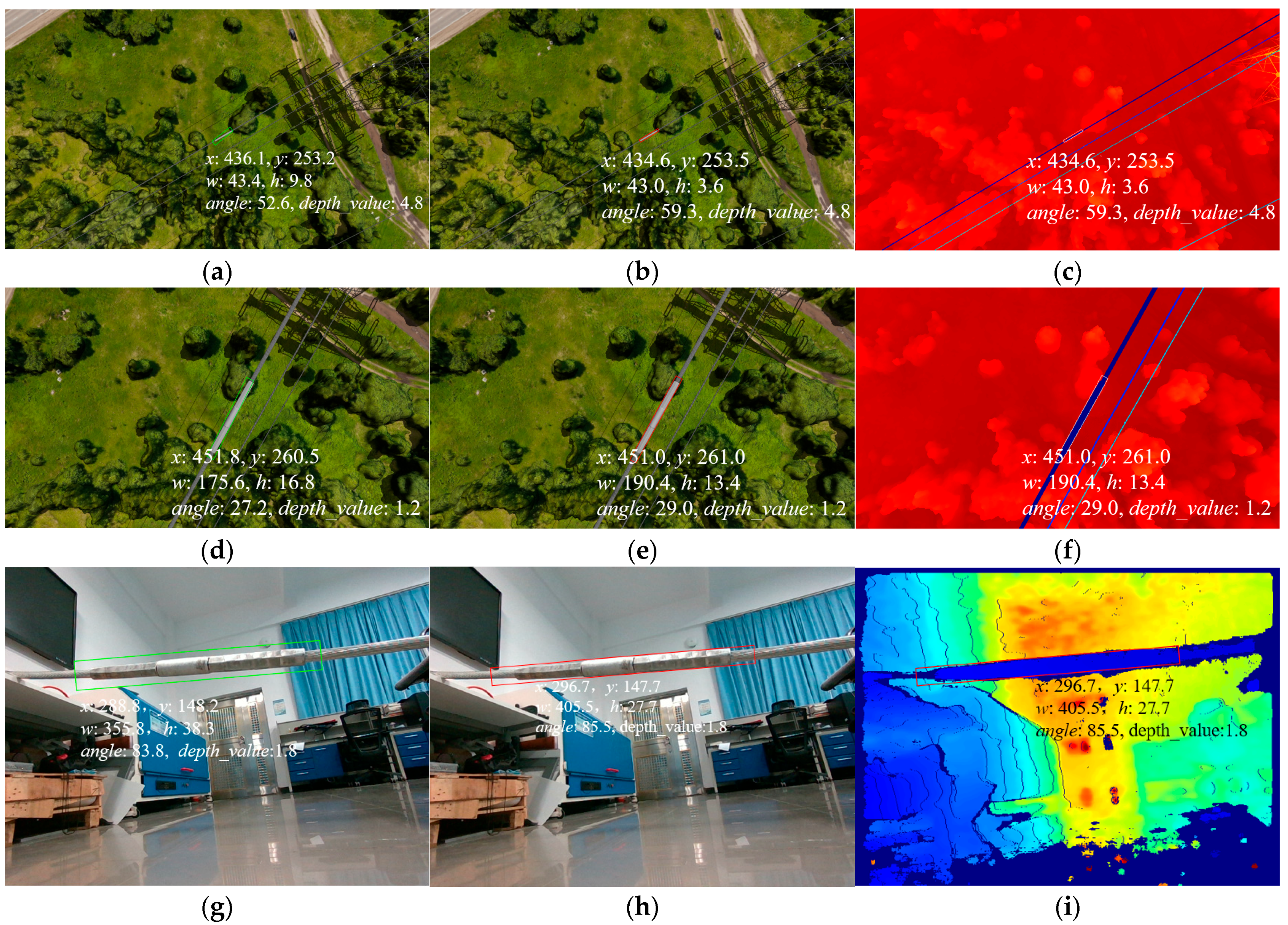
4.1.3. LC Rotational Object Detection Fine Localization Experiment
4.2. UAV-ASS Visual Simulation Experiment Series
4.2.1. UAV-ASS Visual Simulation Platform
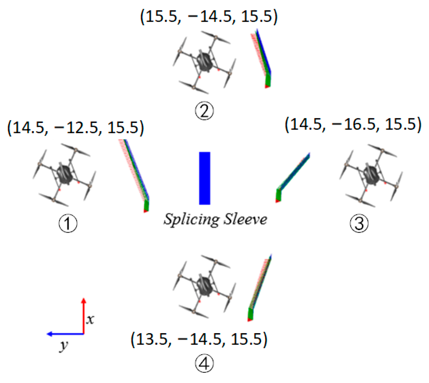
4.2.2. UAV Fixed-Point Rotation Impact on DUAV-SS Experiment
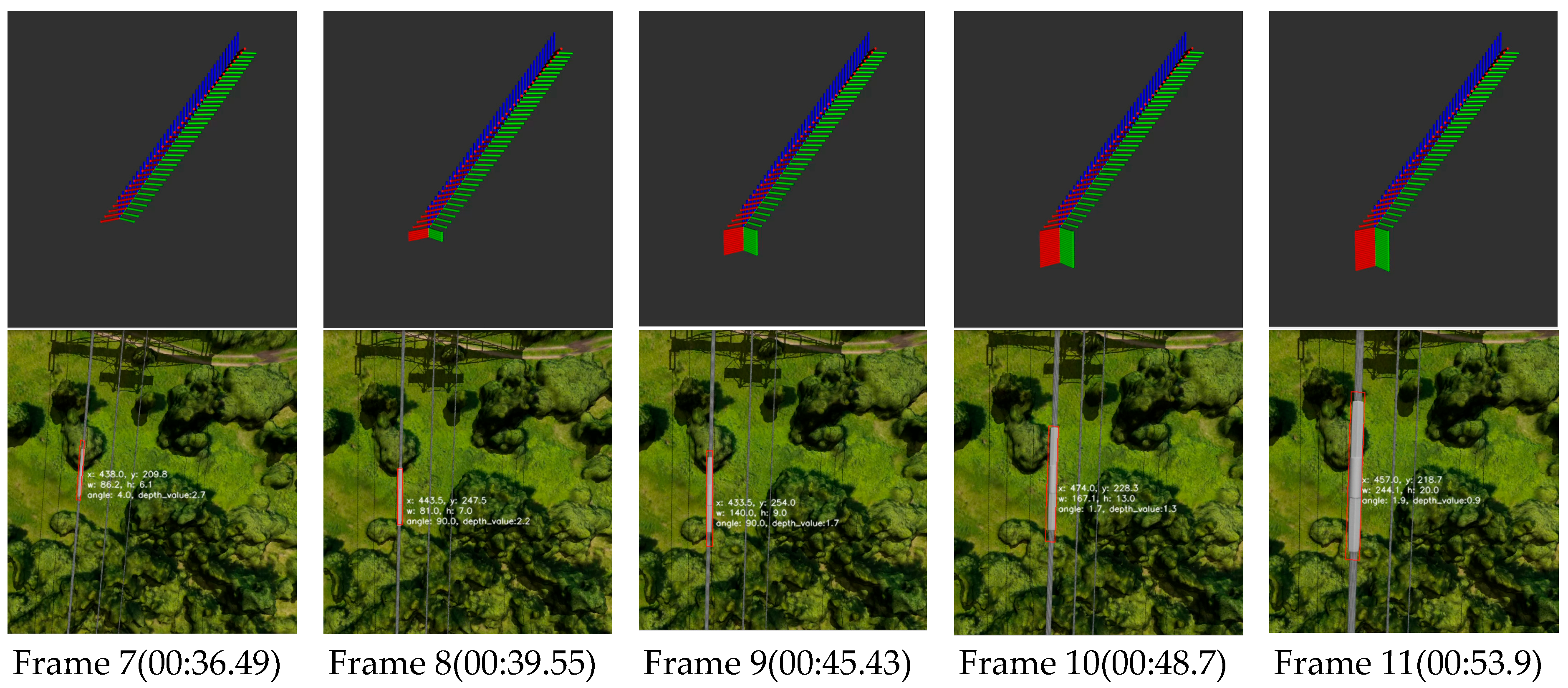
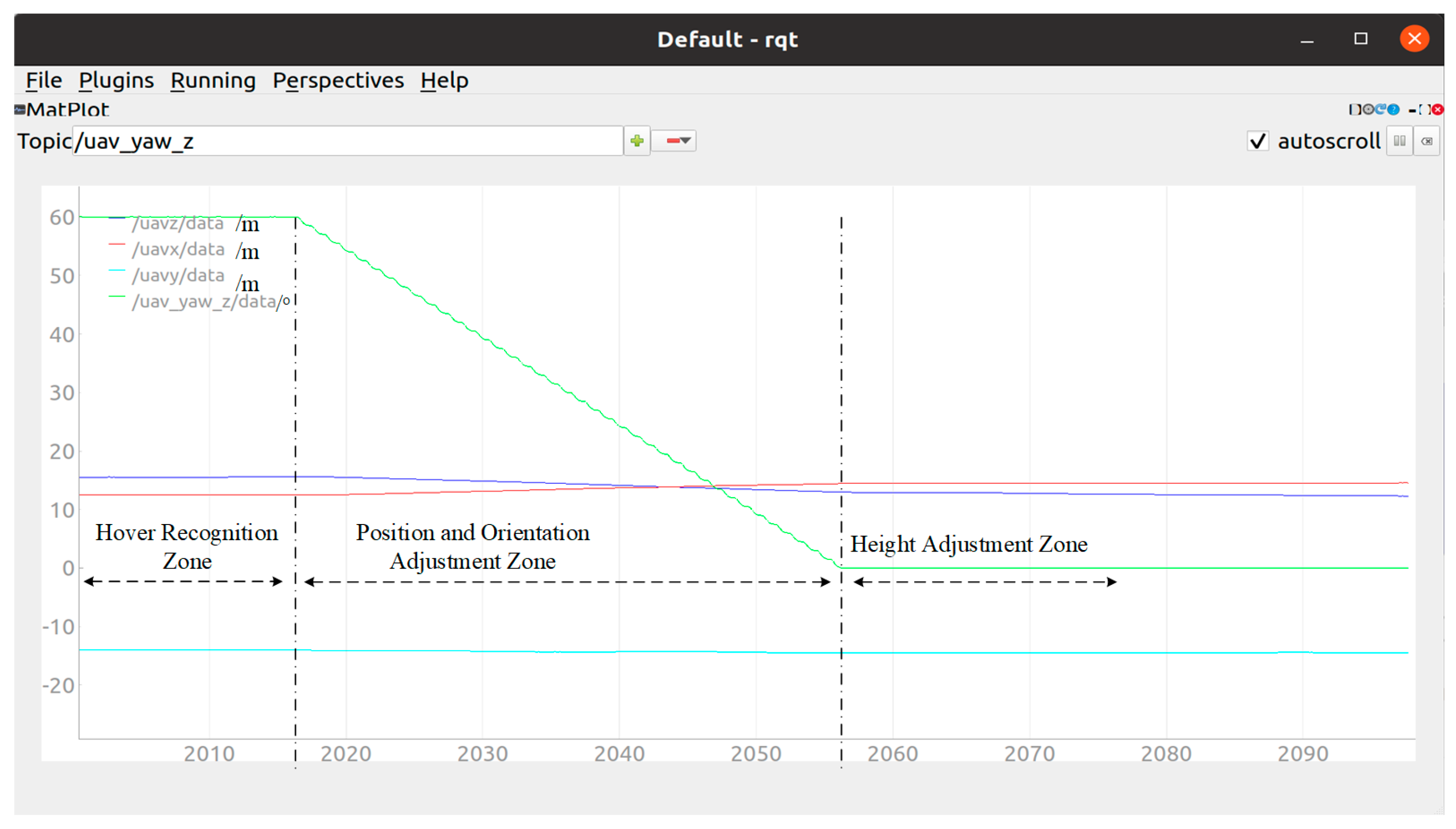
4.2.3. UAV-ASS Waypoint Planning and Docking Experiment
5. Conclusions and Future Works
- (1)
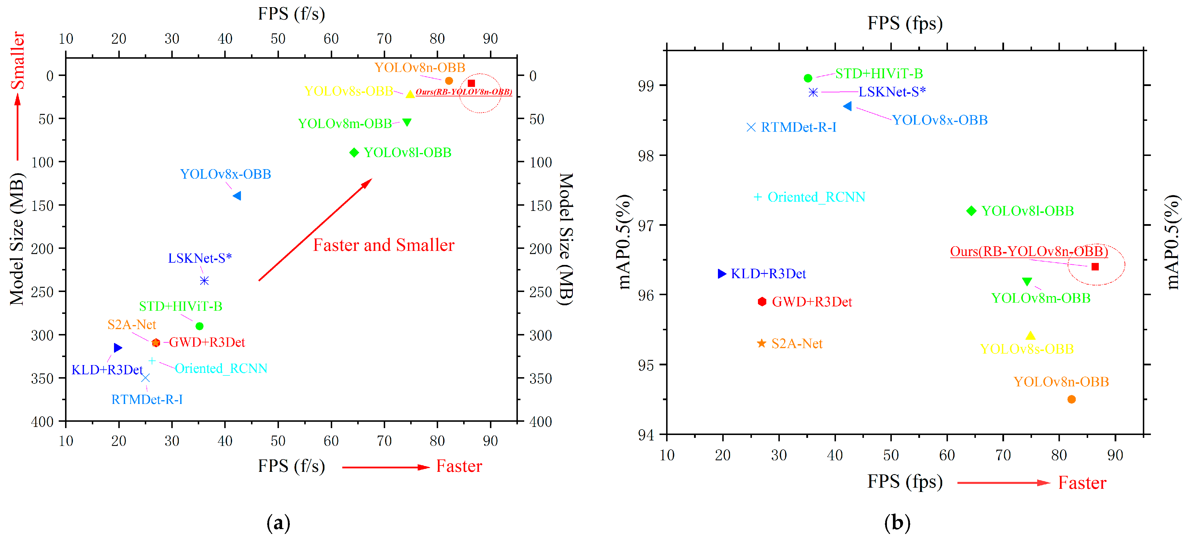
- An algorithm based on the LC-RB-YOLOv8n(OBB) framework was designed specifically for linear target splicing sleeves. This algorithm employs a two-stage localization strategy, achieving rapid and precise localization of splicing sleeves with high reliability. The recognition model within this algorithm attains an average detection accuracy (mAP0.5) of 96.4% and an image inference speed of 86.41 f/s, meeting the real-time and lightweight requirements for high-altitude UAV detection. Additionally, the algorithm integrates depth images of splicing sleeves and performs local clustering analysis of depth values to further enhance the accuracy and reliability of sleeve localization. This algorithm provides a valuable reference for UAV autonomous recognition and docking with linear targets.
- (2)
- Typical virtual scenarios of splicing sleeves containing linear targets were constructed using the 3D modeling software Blender 3.6 to expand the dataset. This approach addresses the high cost and safety risks associated with capturing images of high-altitude transmission line splicing sleeves. It also improves the robustness and generalization ability of the model, providing a valuable reference for constructing deep learning datasets for aerial key targets in the power industry.
- (3)
- Utilizing the open-source PX4 UAV flight control platform, the Robot Operating System (ROS), and the Gazebo physics simulation platform, a UAV-ASS visual simulation platform was developed to quickly validate high-risk algorithms for UAV autonomous recognition and approach of overhead transmission line splicing sleeves. This platform provides an efficient simulation validation tool for high-altitude UAV operations in the power industry, effectively reducing testing costs and safety risks.
Supplementary Materials
Author Contributions
Funding
Data Availability Statement
Acknowledgments
Conflicts of Interest
Abbreviations
| Abbreviation | Full Form/Explanation |
| UAV | Unmanned Aerial Vehicle |
| ASS | Approach Splicing Sleeve |
| SS | Splicing Sleeve |
| OBB | Oriented Bounding Box |
| ROS | Robot Operating System |
| UAV-ASS | UAV approach splicing sleeve |
| mAP | mean Average Precision |
| MRE | Mean Relative Error |
| DR | Digital Radiography |
| GPS | Global Positioning System |
| INS | Inertial Navigation System |
| LiDAR | Light Detection and Ranging |
| IMU | Inertial Measurement Unit |
| UWB | Ultra Wideband |
| GNSS | Global Navigation Satellite System |
| LC | Local Clustering |
| RB | Reparameterization Block |
| RB-YOLOv8(OBB) | A fast rotational object detection model for SS, after reparameterization with the RB module |
| LC-RB-YOLOv8(OBB) | RB-YOLOv8(OBB) model integrated with depth information and local clustering (LC) method |
| RepBlock | Reparameterization Block |
| PAN | Path Aggregation Network |
| FPN | Feature Pyramid Network |
| BN | Batch Normalization |
| Conv | Convolutional Layer |
| Conveq | Equivalent Convolutional Layer |
| Dreal | The real splicing sleeve dataset |
| Dvr | The virtual reality scene splicing sleeve dataset |
| Dau | The augmented splicing sleeve dataset |
| DSS | The splicing sleeve dataset |
| FPS | Frames Per Second |
| MAE | Mean Absolute Error |
| RMSE | Root Mean Squared Error |
| Els | Evaluation Metrics |
| BC_RGB | The detection results of splicing sleeves using the RB-YOLOv8(OBB) model in RGB images |
| BR_Depth | The detection results of splicing sleeves using clustering and minimum area rectangle in local areas (rotation box fitting) |
| BF_RGB | The detection results of splicing sleeves using LC-RB-YOLOv8(OBB) in RGB images |
| BF_Depth | The detection results of splicing sleeves using LC-RB-YOLOv8(OBB) in depth images |
| BC_Depth | The detection results of splicing sleeves using RB-YOLOv8(OBB) in depth images |
| ρC_RGB | The correlation coefficient between the detection results using RB-YOLOv8(OBB) and manually labeled results in RGB images |
| ρF_RGB | The correlation coefficient between the detection results using LC-RB-YOLOv8(OBB) and manually labeled results in RGB images |
| DUAV-SS | UAV’s relative distance to the splicing sleeve |
References
- Liu, Z.; Wu, G.; He, W.; Fan, F.; Ye, X. Key target and defect detection of high-voltage power transmission lines with deep learning. Int. J. Electr. Power Energy Syst. 2022, 142, 108277. [Google Scholar] [CrossRef]
- Wong, S.Y.; Choe, C.W.C.; Goh, H.H.; Low, Y.W.; Cheah, D.Y.S.; Pang, C. Power Transmission Line Fault Detection and Diagnosis Based on Artificial Intelligence Approach and its Development in UAV: A Review. Arab. J. Sci. Eng. 2021, 46, 9305–9331. [Google Scholar] [CrossRef]
- Liu, K.; Li, B.; Qin, L.; Li, Q.; Zhao, F.; Wang, Q.; Xu, Z.; Yu, J. Review of application research of deep learning object detection algorithms in insulator defect detection of overhead transmission lines. High Volt. Eng. 2023, 49, 3584–3595. [Google Scholar] [CrossRef]
- Qin, W.; Yu, G.; Yu, C.; Zhu, K.; Liang, J.; Liu, T. Research on Electromagnetic Interference Protection of X-ray Detecting Device for Tension Clamp of Transmission Line. In Proceedings of the 2022 7th Asia Conference on Power and Electrical Engineering (ACPEE), Hangzhou, China, 15–17 April 2022; pp. 1436–1440. [Google Scholar]
- Liu, Y.; Zhao, P.; Qin, X.; Liu, Y.; Tao, Y.; Jiang, S.; Li, Y. Research on X-ray In-situ Image Processing Technology for Electric Power Strain Clamp. In Proceedings of the Conference on AOPC—Optical Sensing and Imaging Technology, Beijing, China, 20–22 June 2021. [Google Scholar]
- Li, J.; Chen, D.; Li, J.; Zeng, C. Live detection method of transmission line piezoelectric tube defects based on UAV. In Proceedings of the Third International Conference on Artificial Intelligence and Computer Engineering (ICAICE 2022), Wuhan, China, 4–6 November 2022; pp. 41–46. [Google Scholar]
- Luo, D.; Shao, J.; Xu, Y.; Zhang, J. Docking navigation method for UAV autonomous aerial refueling. Sci. China Inf. Sci. 2018, 62, 10203. [Google Scholar] [CrossRef]
- Gong, K.; Liu, B.; Xu, X.; Xu, Y.; He, Y.; Zhang, Z.; Rasol, J. Research of an Unmanned Aerial Vehicle Autonomous Aerial Refueling Docking Method Based on Binocular Vision. Drones 2023, 7, 433. [Google Scholar] [CrossRef]
- Bacelar, T.; Madeiras, J.; Melicio, R.; Cardeira, C.; Oliveira, P. On-board implementation and experimental validation of collaborative transportation of loads with multiple UAVs. Aerosp. Sci. Technol. 2020, 107, 106284. [Google Scholar] [CrossRef]
- Miao, Y.; Tang, Y.; Alzahrani, B.A.; Barnawi, A.; Alafif, T.; Hu, L. Airborne LiDAR Assisted Obstacle Recognition and Intrusion Detection Towards Unmanned Aerial Vehicle: Architecture, Modeling and Evaluation. IEEE Trans. Intell. Transp. Syst. 2020, 22, 4531–4540. [Google Scholar] [CrossRef]
- Huang, J.; He, W.; Yao, Y. Multifiltering Algorithm for Enhancing the Accuracy of Individual Tree Parameter Extraction at Eucalyptus Plantations Using LiDAR Data. Forests 2023, 15, 81. [Google Scholar] [CrossRef]
- Wang, Z.-H.; Chen, W.-J.; Qin, K.-Y. Dynamic Target Tracking and Ingressing of a Small UAV Using Monocular Sensor Based on the Geometric Constraints. Electronics 2021, 10, 1931. [Google Scholar] [CrossRef]
- Meng, X.; Xi, H.; Wei, J.; He, Y.; Han, J.; Song, A. Rotorcraft aerial vehicle’s contact-based landing and vision-based localization research. Robotica 2022, 41, 1127–1144. [Google Scholar] [CrossRef]
- Luo, S.; Liang, Y.; Luo, Z.; Liang, G.; Wang, C.; Wu, X. Vision-Guided Object Recognition and 6D Pose Estimation System Based on Deep Neural Network for Unmanned Aerial Vehicles towards Intelligent Logistics. Appl. Sci. 2022, 13, 115. [Google Scholar] [CrossRef]
- Li, D.; Sun, X.; Elkhouchlaa, H.; Jia, Y.; Yao, Z.; Lin, P.; Li, J.; Lu, H. Fast detection and location of longan fruits using UAV images. Comput. Electron. Agric. 2021, 190, 106465. [Google Scholar] [CrossRef]
- Wang, G.; Qiu, G.; Zhao, W.; Chen, X.; Li, J. A real-time visual compass from two planes for indoor unmanned aerial vehicles (UAVs). Expert Syst. Appl. 2023, 229, 120390. [Google Scholar] [CrossRef]
- Rueda-Ayala, V.P.; Peña, J.M.; Höglind, M.; Bengochea-Guevara, J.M.; Andújar, D. Comparing UAV-Based Technologies and RGB-D Reconstruction Methods for Plant Height and Biomass Monitoring on Grass Ley. Sensors 2019, 19, 535. [Google Scholar] [CrossRef]
- Cao, Z.; Kooistra, L.; Wang, W.; Guo, L.; Valente, J. Real-Time Object Detection Based on UAV Remote Sensing: A Systematic Literature Review. Drones 2023, 7, 620. [Google Scholar] [CrossRef]
- Marelli, D.; Bianco, S.; Ciocca, G. IVL-SYNTHSFM-v2: A synthetic dataset with exact ground truth for the evaluation of 3D reconstruction pipelines. Data Brief 2019, 29, 105041. [Google Scholar] [CrossRef] [PubMed]
- Jia, Z.; Ouyang, Y.; Feng, C.; Fan, S.; Liu, Z.; Sun, C. A Live Detecting System for Strain Clamps of Transmission Lines Based on Dual UAVs’ Cooperation. Drones 2024, 8, 333. [Google Scholar] [CrossRef]
- Ma, Y.; Li, Q.; Chu, L.; Zhou, Y.; Xu, C. Real-Time Detection and Spatial Localization of Insulators for UAV Inspection Based on Binocular Stereo Vision. Remote. Sens. 2021, 13, 230. [Google Scholar] [CrossRef]
- Haque, A.; Elsaharti, A.; Elderini, T.; Elsaharty, M.A.; Neubert, J. UAV Autonomous Localization Using Macro-Features Matching with a CAD Model. Sensors 2020, 20, 743. [Google Scholar] [CrossRef] [PubMed]
- Daramouskas, I.; Meimetis, D.; Patrinopoulou, N.; Lappas, V.; Kostopoulos, V.; Kapoulas, V. Camera-Based Local and Global Target Detection, Tracking, and Localization Techniques for UAVs. Machines 2023, 11, 315. [Google Scholar] [CrossRef]
- Lu, K.; Xu, R.; Li, J.; Lv, Y.; Lin, H.; Liu, Y. A Vision-Based Detection and Spatial Localization Scheme for Forest Fire Inspection from UAV. Forests 2022, 13, 383. [Google Scholar] [CrossRef]
- Arafat, M.Y.; Alam, M.M.; Moh, S. Vision-Based Navigation Techniques for Unmanned Aerial Vehicles: Review and Challenges. Drones 2023, 7, 89. [Google Scholar] [CrossRef]
- Cheng, C.; Li, X.; Xie, L.; Li, L. Autonomous dynamic docking of UAV based on UWB-vision in GPS-denied environment. J. Frankl. Inst. 2022, 359, 2788–2809. [Google Scholar] [CrossRef]
- Li, Z.; Tian, Y.; Yang, G.; Li, E.; Zhang, Y.; Chen, M.; Liang, Z.; Tan, M. Vision-Based Autonomous Landing of a Hybrid Robot on a Powerline. IEEE Trans. Instrum. Meas. 2022, 72, 1–11. [Google Scholar] [CrossRef]
- Chen, C.; Chen, S.; Hu, G.; Chen, B.; Chen, P.; Su, K. An auto-landing strategy based on pan-tilt based visual servoing for unmanned aerial vehicle in GNSS-denied environments. Aerosp. Sci. Technol. 2021, 116, 106891. [Google Scholar] [CrossRef]
- Zhou, Y.; Zhang, D.; Ma, X. Distribution network insulator detection based on improved ant colony algorithm and deep learning for UAV. iScience 2024, 27, 110119. [Google Scholar] [CrossRef] [PubMed]
- Chang, Y.; Cheng, Y.; Manzoor, U.; Murray, J. A review of UAV autonomous navigation in GPS-denied environments. Robot. Auton. Syst. 2023, 170, 104533. [Google Scholar] [CrossRef]
- Feng, S.; Huang, Y.; Zhang, N. An Improved YOLOv8 OBB Model for Ship Detection through Stable Diffusion Data Augmentation. Sensors 2024, 24, 5850. [Google Scholar] [CrossRef]
- Xia, G.-S.; Bai, X.; Ding, J.; Zhu, Z.; Belongie, S.; Luo, J.; Datcu, M.; Pelillo, M.; Zhang, L. DOTA: A Large-scale Dataset for Object Detection in Aerial Images. In Proceedings of the 31st IEEE/CVF Conference on Computer Vision and Pattern Recognition (CVPR), Salt Lake City, UT, USA, 18–23 June 2018; pp. 3974–3983. [Google Scholar]
- Li, R.; Shao, Z.; Zhang, X. Rep2former: A classification model enhanced via reparameterization and higher-order spatial interactions. J. Electron. Imaging 2023, 32, 053002. [Google Scholar] [CrossRef]
- Lloyd, S.P. Least squares quantization in PCM. IEEE Trans. Inf. Theory 1982, 28, 129–137. [Google Scholar] [CrossRef]
- Ren, Z.; Lin, T.; Feng, K.; Zhu, Y.; Liu, Z.; Yan, K. A Systematic Review on Imbalanced Learning Methods in Intelligent Fault Diagnosis. IEEE Trans. Instrum. Meas. 2023, 72, 1–35. [Google Scholar] [CrossRef]
- Meng, Q.; Zheng, W.; Xue, P.; Xin, Z.; Liu, C. Research and application of CNN-based transmission line hazard identification technology. In Proceedings of the Annual Meeting of CSEE Study Committee of HVDC and Power Electronics (HVDC 2023), Nanjing, China, 22–25 October 2023; pp. 296–300. [Google Scholar]
- Liu, J.; Jia, R.; Li, W.; Ma, F.; Wang, X. Image Dehazing Method of Transmission Line for Unmanned Aerial Vehicle Inspection Based on Densely Connection Pyramid Network. Wirel. Commun. Mob. Comput. 2020, 2020, 8857271. [Google Scholar] [CrossRef]
- Dong, C.; Zhang, K.; Xie, Z.; Shi, C. An improved cascade RCNN detection method for key components and defects of transmission lines. IET Gener. Transm. Distrib. 2023, 17, 4277–4292. [Google Scholar] [CrossRef]
- Yu, H.; Tian, Y.; Ye, Q.; Liu, Y. Spatial Transform Decoupling for Oriented Object Detection. arXiv 2024, arXiv:2308.10561. [Google Scholar] [CrossRef]
- Li, Y.; Hou, Q.; Zheng, Z.; Cheng, M.M.; Yang, J.; Li, X. Large Selective Kernel Network for Remote Sensing Object Detection. In Proceedings of the IEEE/CVF International Conference on Computer Vision 2023, Paris, France, 2–3 October 2023; pp. 16748–16759. [Google Scholar]
- Lyu, C.; Zhang, W.; Huang, H.; Zhou, Y.; Wang, Y.; Liu, Y.; Zhang, S.; Chen, K. RTMDet: An Empirical Study of Designing Real-Time Object Detectors. arXiv 2022, arXiv:2212.07784. [Google Scholar]
- Yang, X.; Yang, X.; Yang, J.; Ming, Q.; Wang, W.; Tian, Q.; Yan, J. Learning High-Precision Bounding Box for Rotated Object Detection via Kullback-Leibler Divergence. In Proceedings of the 35th Conference on Neural Information Processing Systems (NeurIPS), Electr Network, Online, 6–14 December 2021. [Google Scholar]
- Xue, Y.; Junchi, Y.; Qi, M.; Wentao, W.; Xiaopeng, Z.; Qi, T. Rethinking Rotated Object Detection with Gaussian Wasserstein Distance Loss. arXiv 2021, arXiv:2101.11952. [Google Scholar]
- Jiaming, H.; Jian, D.; Jie, L.; Gui-Song, X. Align deep features for oriented object detection. IEEE Trans. Geosci. Remote Sens. 2021, 60, 5602511. [Google Scholar]
- Xie, X.; Cheng, G.; Wang, J.; Yao, X.; Han, J. Oriented R-CNN for Object Detection. In Proceedings of the 18th IEEE/CVF International Conference on Computer Vision (ICCV), Electr Network, Online, 11–17 October 2021; pp. 3500–3509. [Google Scholar]
- Jocher, G.; Chaurasia, A.; Oiu, J. YOLO by Ultralytics. Available online: https://github.com/ultralytics/ultralytics (accessed on 4 July 2024).
- Ruiz, F.; Arrue, B.C.; Ollero, A. SOPHIE: Soft and Flexible Aerial Vehicle for Physical Interaction with the Environment. IEEE Robot. Autom. Lett. 2022, 7, 11086–11093. [Google Scholar] [CrossRef]
- Zufferey, R.; Barbero, J.T.; Talegon, D.F.; Nekoo, S.R.; Acosta, J.A.; Ollero, A. How ornithopters can perch autonomously on a branch. Nat. Commun. 2022, 13, 7713. [Google Scholar] [CrossRef]


| Study | Target Type | Depth Sensing Method | Algorithm | Key Contribution |
|---|---|---|---|---|
| Jia et al. [20] | Overhead clamp | Passive stereo vision | YOLOv8n + 3D coordinate detection | Real-time distance measurement between UAV and clamp to ensure safety. |
| Li et al. [21] | Insulator | RGB-D depth detection | RGB-D saliency detection | Combines real-time flight data to locate insulators’ longitude, latitude, and altitude. |
| Elsaharti et al. [22] | Indoor target | Passive stereo vision + CAD model matching | Real-time macro feature vector matching | Matches features captured by UAV to pre-stored CAD models for rapid indoor localization. |
| Daramouskas et al. [23] | General targets | Multi-camera localization | Improved YOLOv4 + multi-camera fusion | Introduces multi-camera-based detection for improved precision and tracking. |
| Li et al. [24] | Fire objects | Passive stereo vision | HSV-Mask filtering + non-zero mean method | Detects fire areas, computes depth, and combines GPS/IMU data for geographical localization. |
| Li et al. [15] | Longan fruits | Active stereo vision(D455) | MobileNet + YOLOv4 | Improves the speed and accuracy of target detection and location for longan picking by UAVs based on vision. |
| This study | Overhead splicing sleeves | Active stereo vision | LC-RB-YOLOv8n(OBB) | Addresses the problem of rapid recognition and precise distance measurement for UAV docking with linear targets. |
| Study | Target Scenario | Sensor Type | Algorithm | Key Contribution |
|---|---|---|---|---|
| Li et al. [26] | Docking with moving platforms | UWB + vision sensors | Integrated estimation and control | Proposed a three-stage hovering, approaching, and landing control method for UAV docking. |
| Yang et al. [27] | Powerline inspection | Stereo vision | Feature extraction + depth measurement | Combined UAV and climbing robots for multi-scale powerline inspection, enabling stable landing. |
| Chen et al. [28] | GNSS-denied environment | Omnidirectional camera + gimbal system | Image-guided landing control | Guided UAV landing on a square platform in GNSS-denied conditions with stage-specific strategies. |
| Zhou et al. [29] | Overhead line inspection | Camera + deep learning | Improved ant colony algorithm + defect detection | Introduced UAV path planning and visual inspection, significantly improving inspection efficiency. |
| This study | Overhead splicing sleeves | Active stereo vision | LC-RB-YOLOv8n(OBB) + virtual simulation | Proposes a deep learning and active stereo vision-based docking method, solving angular measurement challenges. |
| Rotating Target Detection Model | Precision (%) | Recall (%) | mAP0.5 (%) | Spend (ms/img) | FPS (f/s) | Model Size (MB) |
|---|---|---|---|---|---|---|
| Ours | 96.7 | 95.7 | 96.4 | 11.57 | 86.41 | 9.4 |
| YOLOv8n-OBB [46] | 98.8 | 88.2 | 94.5 | 12.17 | 82.17 | 6.6 |
| YOLOv8s-OBB [46] | 95.8 | 87.8 | 95.4 | 13.35 | 74.91 | 23.3 |
| YOLOv8m-OBB [46] | 96.2 | 92.5 | 96.2 | 13.47 | 74.24 | 53.3 |
| YOLOv8l-OBB [46] | 98.4 | 93.9 | 97.2 | 15.54 | 64.35 | 89.5 |
| YOLOv8x-OBB [46] | 98.8 | 94.6 | 98.7 | 23.58 | 42.41 | 139.5 |
| KLD+R3Det t [42] | 95.8 | 93.5 | 96.3 | 50.92 | 19.64 | 315.3 |
| GWD+R3Det [43] | 95.2 | 90.1 | 95.9 | 37.04 | 27.00 | 309.5 |
| S2A-Net [44] | 94.3 | 93 | 95.3 | 37.17 | 26.90 | 309.6 |
| Oriented_RCNN [45] | 98.3 | 92.6 | 97.4 | 38.14 | 26.22 | 330.3 |
| STD+HIViT-B [39] | 99.0 | 98.5 | 99.1 | 28.41 | 35.20 | 290.5 |
| LSKNet-S* [40] | 97.2 | 96.5 | 98.9 | 27.70 | 36.10 | 237.6 |
| RTMDet-R-I [41] | 93.4 | 95.2 | 98.4 | 39.97 | 25.02 | 350.1 |
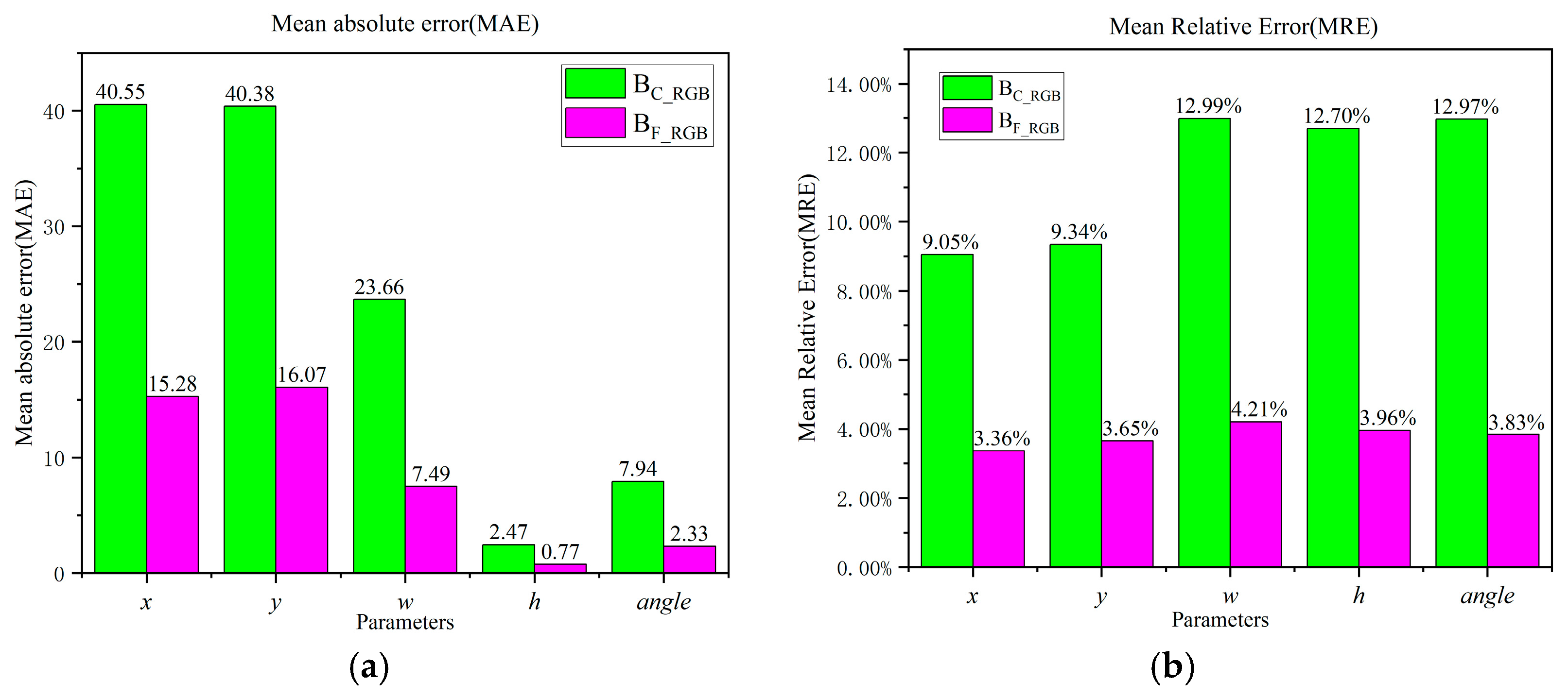
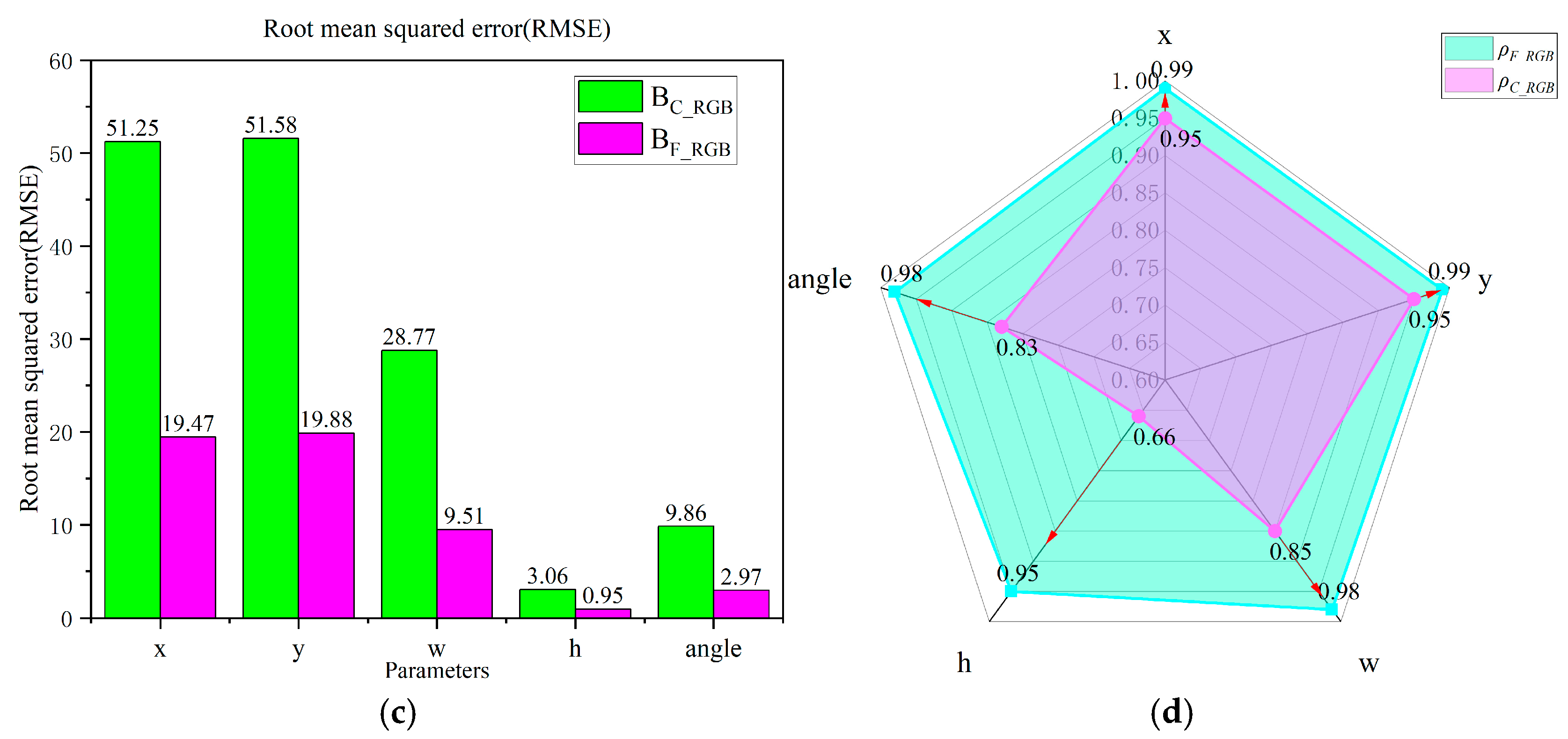
| Model | BC_RGB | BF_RGB | |||||||
|---|---|---|---|---|---|---|---|---|---|
| Els | MAE | MRE | RMSE | ρ | MAE | MRE | RMSE | ρ | |
| Parameters | |||||||||
| x | 40.55 | 9.05% | 51.25 | 0.95 | 15.28 | 3.39% | 19.47 | 0.99 | |
| y | 40.38 | 9.34% | 51.58 | 0.95 | 16.07 | 3.65% | 19.88 | 0.99 | |
| w | 23.66 | 12.99% | 28.77 | 0.85 | 7.49 | 4.21% | 9.51 | 0.98 | |
| h | 2.47 | 12.7% | 3.06 | 0.66 | 0.77 | 3.96% | 0.95 | 0.95 | |
| angle | 7.94 | 12.97% | 9.86 | 0.83 | 2.33 | 3.83% | 2.97 | 0.98 | |
| Location Error | X-Axis Error/m | Y-Axis Error/m | Z-Axis Error/m | Angle Error/° | |
|---|---|---|---|---|---|
| Starting Position | |||||
| ① (14.5 m, −12.5 m, 15.5 m) | −0.05 | +0.06 | −0.07 | 2 | |
| ② (15.5 m, −14.5 m, 15.5 m) | +0.03 | +0.03 | −0.06 | 3 | |
| ③ (14.5 m, −16.5 m, 15.5 m) | −0.05 | +0.06 | +0.04 | −4 | |
| ④ (13.5 m, −14.5 m, 15.5 m) | +0.07 | +0.05 | −0.06 | 2 | |
| MAE | 0.050 | 0.050 | 0.058 | 2.750 | |
Disclaimer/Publisher’s Note: The statements, opinions and data contained in all publications are solely those of the individual author(s) and contributor(s) and not of MDPI and/or the editor(s). MDPI and/or the editor(s) disclaim responsibility for any injury to people or property resulting from any ideas, methods, instructions or products referred to in the content. |
© 2024 by the authors. Licensee MDPI, Basel, Switzerland. This article is an open access article distributed under the terms and conditions of the Creative Commons Attribution (CC BY) license (https://creativecommons.org/licenses/by/4.0/).
Share and Cite
Zhang, G.; Liu, G.; Zhong, F. Research on UAV Autonomous Recognition and Approach Method for Linear Target Splicing Sleeves Based on Deep Learning and Active Stereo Vision. Electronics 2024, 13, 4872. https://doi.org/10.3390/electronics13244872
Zhang G, Liu G, Zhong F. Research on UAV Autonomous Recognition and Approach Method for Linear Target Splicing Sleeves Based on Deep Learning and Active Stereo Vision. Electronics. 2024; 13(24):4872. https://doi.org/10.3390/electronics13244872
Chicago/Turabian StyleZhang, Guocai, Guixiong Liu, and Fei Zhong. 2024. "Research on UAV Autonomous Recognition and Approach Method for Linear Target Splicing Sleeves Based on Deep Learning and Active Stereo Vision" Electronics 13, no. 24: 4872. https://doi.org/10.3390/electronics13244872
APA StyleZhang, G., Liu, G., & Zhong, F. (2024). Research on UAV Autonomous Recognition and Approach Method for Linear Target Splicing Sleeves Based on Deep Learning and Active Stereo Vision. Electronics, 13(24), 4872. https://doi.org/10.3390/electronics13244872