Adaptive Traffic Signal Control Based on Graph Neural Networks and Dynamic Entropy-Constrained Soft Actor–Critic

Abstract

Traffic congestion remains a significant challenge in urban management, with traditional fixed-cycle traffic signal systems struggling to adapt to dynamic traffic conditions. This paper proposes an adaptive traffic signal control method based on a Graph Neural Network (GNN) and a dynamic entropy-constrained Soft Actor–Critic (DESAC) algorithm. The approach first extracts both global and local features of the traffic network using GNN and then utilizes the DESAC algorithm to optimize traffic signal control at both single and multi-intersection levels. Finally, a simulation environment is established on the CityFlow platform to evaluate the proposed method’s performance through experiments involving single and twelve intersection scenarios. Simulation results on the CityFlow platform demonstrate that G-DESAC significantly improves traffic flow, reduces delays and queue lengths, and enhances intersection capacity compared to other algorithms. In single intersection scenarios, G-DESAC achieves a higher reward, reduced total delay time, minimized queue lengths, and improved throughput. In multi-intersection scenarios, G-DESAC maintains high rewards with stable and efficient optimization, outperforming DQN, SAC, Max-Pressure, and DDPG. This research highlights the potential of deep reinforcement learning (DRL) in urban traffic management and positions G-DESAC as a robust solution for practical traffic signal control applications, offering substantial improvements in traffic efficiency and congestion mitigation.

1. Introduction

Traffic congestion not only disrupts mobility but also incurs significant socio-economic costs, including increased fuel consumption, increased air pollution, and decreased productivity. Effectively managing traffic flow to alleviate congestion is a critical challenge for modern transportation systems. Traditional fixed-cycle signal control lacks the flexibility needed to adapt to dynamic traffic conditions, and it fails to optimize traffic flow at a broader, network-wide level. Adjustments made at a single intersection may inadvertently disrupt surrounding areas, highlighting the need for a more integrated approach. As urbanization and vehicle numbers continue to rise, improving traffic signal efficiency has become crucial. Expanding road capacity or optimizing existing infrastructure are common strategies, but road expansion is costly, and it can have limited long-term effects. According to the “Law of Peak-Hour Expressway Congestion”, additional road capacity is often quickly consumed by rising demand, meaning congestion persists. Consequently, enhancing the efficiency of existing traffic signal control systems presents a more effective, sustainable solution. This paper proposes the use of artificial intelligence techniques [1] to design an adaptive traffic signal controller.

Traditional traffic signal systems, based on fixed timing sequences, struggle to respond to real-time fluctuations in traffic flow. Recent advancements in adaptive control, such as genetic algorithms, population intelligence, and neural networks, have attempted to address this issue. However, these methods often rely on models and historical data [2], which can overlook short-term variations and spatial distribution differences. In contrast, model-free [3] reinforcement learning (RL) [4], particularly deep reinforcement learning (DRL), offers significant potential for optimizing traffic signal control. By learning optimal strategies through interaction with the environment, RL avoids reliance on fixed parameters and adapts to real-time changes. RL has already been successfully applied in various domains [5], including traffic signal optimization, driving behavior analysis, and fluctuation prediction. In the context of traffic signal control, the application framework for reinforcement learning is shown in Figure 1. In this framework, the environment consists of the current traffic flow and the phases of the signals. The signal phase in traffic signal control refers to the authority to release a particular traffic flow during a signal cycle. The state represents features, such as vehicle queue lengths or waiting times, and the agent learns a strategy to select actions (e.g., maintaining or switching signal phases) based on these features. The agent’s actions are evaluated through rewards, with the aim of maximizing cumulative rewards over time. This dynamic interaction allows RL to overcome some of the key limitations of traditional model-based approaches.

Recent research in traffic management has expanded our understanding of congestion and its control. In this study, congestion refers to a condition where vehicles experience prolonged queuing times and reduced travel speeds on the road. This clear definition allows for precise identification and measurement of traffic congestion, offering a reliable foundation for effective traffic management and planning. Tsuboi [6], through extensive observations in India, introduced the concept of congestion “gap”, demonstrating that detailed monitoring of traffic patterns and environmental factors can significantly enhance traffic management strategies. Similarly, Yue [7] focused on the progression of congestion control methods, emphasizing the critical role of traffic signal optimization. Advances in sensing, communication, and computation have facilitated more effective mitigation of congestion. Yue [8] further developed techniques to identify and predict the root causes of traffic congestion, employing certain tools, such as causal congestion trees, Markov models, and gradient boosting. These methods were rigorously tested through simulations and validated with real-world data from Taipei, underscoring their practical applicability.

This paper proposes an adaptive traffic signal control method that integrates Graph Neural Networks (GNNs) and the dynamic entropy-constrained Soft Actor–Critic (DESAC) algorithm. By leveraging GNN’s ability to extract graph-based features and DESAC’s capacity for deep reinforcement learning, the method optimizes traffic signal control at both single and multiple intersections in real time, thus enhancing the cooperative control of traffic flow.

The paper is organized as follows: Section 2 reviews existing traffic signal control methods; Section 3 introduces the proposed method; Section 4 describes the experimental setup and parameter settings; and Section 5 presents the experimental results and outlines potential future research directions.

2. Related Research

Numerous studies have been conducted in the field of traffic signal control (TSC) to explore various approaches aimed at improving traffic flow and alleviating congestion. The field’s origins can be traced back to the 1980s with the introduction of the SCATS and SCOOT systems [9]. Early TSC methods were heavily reliant on predefined protocols and statistical flow data [10], but these systems were limited in their ability to adapt to real-time traffic fluctuations.

With the advancement of artificial intelligence (AI), the application of deep reinforcement learning (DRL) in TSC has gained increasing attention. DRL optimizes complex dynamic systems by learning the best control strategies through interactions with the environment, positioning it as a state-of-the-art framework in control systems. Deep learning (DL) methods, which include deep neural networks (DNNs), such as fully connected layer networks (FCLNs) [11], can approximate complex, nonlinear functions [12] by utilizing deep architectures with many hidden layers (e.g., up to 150 layers [13]). This is in contrast to traditional neural networks, which typically consist of fewer layers (e.g., two or three) [14]. DL has had a transformative impact in certain fields, such as image recognition, natural language processing, and autonomous driving [15,16,17]. DRL, as a combination of DL and reinforcement learning (RL), uses neural networks to approximate either a value function or a policy function, effectively handling high-dimensional and continuous state spaces.

Research in DRL-based traffic signal control has seen significant progress. The Deep Q-Network (DQN), introduced by DeepMind [18], was the first DRL method applied to TSC, and it has since become widely adopted. For example, Li et al. [19] developed a DQN-based adaptive traffic signal control model within the SUMO simulation environment, optimizing traffic flow and reducing waiting and travel times. Xie et al. [20] proposed a dynamic information dissemination strategy using double-deep Q-learning (DDQL) to optimize network performance following traffic accidents through real-time data collection and information sharing. Cai et al. [21] integrated dueling networks, double Q-learning, and preferential sampling to enhance training efficiency and model robustness in traffic signal control. Zeinaly et al. [22] developed DRL-driven adaptive signal controllers that quickly respond to accidents, helping to reduce congestion.

Multi-agent deep reinforcement learning (MARL) has also proven effective in TSC. Wang et al. [23] introduced a multi-agent DRL method, SEMA2C, which achieves efficient collaborative control in multi-intersection scenarios through shared experiences and importance sampling. Jung et al. [24] proposed a multi-agent DRL approach that incorporates environmental factors to improve traffic efficiency and reduce greenhouse gas emissions. Chang et al. [25] addressed multi-signal coordination through a communication-enhanced multi-agent DRL method (CVDMARL), which improves performance during peak traffic periods. Additionally, Deng et al. [26] proposed a multi-agent DRL-based ramp control algorithm that optimizes ramp scheduling to improve mainline speed and reduce ramp queue lengths.

Additionally, several studies have focused on enhancing the performance of DRL in traffic signal control (TSC) through data-driven innovations and algorithmic advancements. Xu et al. [27] proposed a data-driven framework for identifying and optimizing key nodes in a traffic network, significantly improving access efficiency and reducing delays. Zhao et al. [28] introduced a heterogeneous Graph Neural Network model that integrates a dual-attention mechanism with DRL, enhancing the scheduling efficiency of intersections. Mao et al. [29] applied the Soft Actor–Critic (SAC) algorithm to TSC for the first time, demonstrating its superior adaptability and performance compared to other methods. Fuad et al. [30] developed an adaptive TSC algorithm based on deep Q-networks, combined with a macro fundamental graph and an exponential rewarding mechanism to significantly improve traffic flow. Zai et al. [31] incorporated an efficient channel attention mechanism, LSTM, and double dominance DQN to enhance cumulative rewards, reduce queue lengths, and lower CO₂ emissions. Zhang et al. [32] proposed an Adaptive Traffic Signal Priority (ATSP) model that integrates single and multiple request modules to optimize the efficiency of both public transport and private vehicles.

To deepen the understanding of traffic congestion, several state-of-the-art studies have analyzed traffic flow dynamics and congestion thresholds. Lee et al. [33]. identified critical congestion points on highways by examining bimodal traffic flow distributions, providing insights into early indicators of congestion. Hollbeck [34] leveraged symmetrized time-lagged correlation matrices to study motorway congestion patterns and durations, uncovering a nonlinear relationship between spectral transitions and congestion persistence. Similarly, Drliciak [35] demonstrated that when road capacity is exceeded, travel speed decreases by 30% for vehicle groups larger than 25, enabling more accurate traffic flow modeling. Laval [36] took a broader perspective by comparing vehicular traffic dynamics to phase transitions in fluids. His network traffic model revealed superlinear scaling of congestion costs with city populations, exceeding predictions by West. These findings carry significant implications for sustainable urban planning and the mitigation of traffic congestion in rapidly growing cities.

In parallel, research has also focused on improving traffic simulators for more efficient modeling. In 1990, Messner and Papageorgiou [37] introduced METANET, a macroscopic traffic simulator capable of maintaining consistent speeds across varying vehicle flows, which is suitable for simulating diverse traffic conditions. In 2005, Barceló and Casas [38] developed AIMSUN, a microscopic simulator known for its excellent performance in large-scale urban simulations. In the same year, Prezioso [39] introduced VISSIM, another microscopic simulator with high efficiency for large-scale urban simulations. In 2018, Lopez et al. [40] presented SUMO, a microscopic simulator that supports urban simulations involving more than 10,000 streets. More recently, in 2019, Zhang et al. [41] developed CityFlow, which enhances simulation efficiency through multi-threading and adapts to traffic networks of various sizes.

In summary, in recent years, the integration of deep reinforcement learning (DRL) into traffic signal control has marked a shift from traditional rule-based approaches to adaptive, intelligent systems. DRL has shown significant potential in optimizing complex dynamic systems, particularly through advancements in multi-agent DRL and data-driven strategies. However, while these methods have achieved some success in traffic signal control (TSC), challenges persist in coordinating traffic across multiple intersections. Traditional DRL approaches struggle to effectively capture the global dynamics of traffic systems, leading to slow convergence, low learning efficiency, and instability in high-dimensional state spaces. Additionally, multi-agent models often rely on local information from individual agents, making it difficult to achieve globally optimized control. Effective coordination among multiple intersections requires a holistic understanding of the entire traffic network, a task beyond the capabilities of single-agent or simplistic multi-agent models.

To address these limitations, this paper introduces an adaptive traffic signal control method based on a combination of Graph Neural Networks (GNNs) and a dynamic entropy-constrained Soft Actor–Critic (DESAC) algorithm. GNNs leverage graph structures to represent intersections and their connectivity, enabling efficient modeling of complex interactions and dynamic behaviors across the traffic network through a message-passing mechanism. The DESAC algorithm enhances decision making by incorporating dynamic entropy constraints, which improve exploration and stabilize policy learning, particularly in high-dimensional state spaces.

The integration of GNNs and DESAC offers dual benefits: it excels in single intersection control while enabling efficient modeling and coordination of multi-intersection traffic systems. This approach significantly improves response speed, adaptability, and traffic signal efficiency. Experimental results from the CityFlow simulation validate its effectiveness, demonstrating substantial improvements in overall traffic flow, reduced vehicle waiting times, enhanced traffic efficiency, and lower carbon emissions. This method leverages intelligent traffic signal optimization to enhance traffic flow and road capacity while significantly improving overall traffic performance. It offers innovative technical support for advancing urban traffic management. These outcomes highlight the method’s practical potential. This paper provides a detailed description of the proposed method’s design and implementation and presents experimental evidence of its superiority in managing complex traffic scenarios.

3. Methodology

3.1. Traffic Signal Control Definition

A traffic network can be represented as a directed graph H = (P, Q), where p ∈ P represents an intersection and $q_{pt}=(p,t)\in Q$ denotes the adjacency and connection between two intersections. The neighborhood of junction p is denoted as ${\mathrm{N}\mathrm{B}}_p=\{t\mid (p,t)\in Q\}$, and the degree of an intersection is the size of its neighborhood. $d(p,t)$ represents the minimum number of sides connecting the two junctions $p$ and $t$. Each intersection has two types of lanes: entrance lanes, where vehicles enter the intersection, and exit lanes, where vehicles leave. An intersection consists of multiple entry and exit lanes. The set of entry lanes at an intersection is denoted as $L_{in}$. Traffic flow is defined as a combination of an entry lane and an exit lane. A phase refers to the combination of traffic flows that are set to green during a signal cycle. For example, as shown in Figure 2, an intersection may have four phases: North–South Straight (NS), North–South Left Turn (NSL), East–West Straight (EW), and East–West Left Turn (EWL).

3.2. The Overall Architecture of the Algorithm

This study proposes an adaptive traffic signal control algorithm based on GNN and the dynamic entropy-constrained Soft Actor–Critic (DESAC) algorithm. The overall framework of the algorithm is shown in Figure 3. The simulation environment and data transfer interconnect the modules, enabling dynamic optimization of traffic signals for both single and multiple intersections. This approach takes into account not only the state of individual intersections but also the broader context of the surrounding intersections. The system consists of several key components.

• Environment Simulation Module (a): The CityFlow platform simulates real-world traffic scenarios using intersection datasets from Hangzhou and Jinan. Traffic state data are obtained, and traffic network graphs are generated primarily through the _get_graph_data method in the CityFlowEnvWithGNN class. In addition to modeling the traffic state at individual intersections, the surrounding intersections are also incorporated into the model through the construction of a traffic network diagram. This enhances the overall traffic signal control strategy, making it more comprehensive and effective. To avoid traffic flow surpassing the critical threshold that leads to congestion, the system may deliberately create vehicle convoys during free-flow conditions, maintaining the flow below this critical point.
• GNN Feature Extraction Module (b): In this module, GNN is used to extract both global and local features of the traffic network from preprocessed data. The GNNFeatureExtractor class implements a simple two-layer Graph Convolutional Network (GCN), where the first layer extracts hidden features from input data using the ReLU activation function and the second layer extracts output features. The graph features are then extracted via the _get_state method in the CityFlowEnvWithGNN class. This feature extraction module captures various aspects, including the following. Node features: traffic-related data for each intersection, such as traffic flow, lane queue length, and vehicle speed. Edge features: information on each road segment, including road length and number of lanes. Spatio-temporal correlations: traffic flow patterns over time, captured through multiple Graph Convolution Layers (GCLs). The final output is a feature vector representing the aggregated information for each intersection, which is used by the decision module to generate signal control strategies. By leveraging graph structure data, the module ensures a more accurate reflection of traffic status. In our study, traffic states are modeled as a graph structure comprising nodes and edges, where each node represents a traffic intersection and edges represent traffic flow between intersections. Using a Graph Neural Network (GNN), we extract high-level features from this graph to capture the spatial and temporal dynamics of the traffic network. These features are integrated with real-time data, such as traffic flow and vehicle speed, within the CityFlowEnvWithGNN module, forming the input states for the reinforcement learning process. This combination allows our model to accurately reflect traffic dynamics, optimizing traffic signal control strategies. Compared to traditional feature extraction methods, GNNs excel in capturing both local and global traffic flow patterns. Traditional methods typically focus on local features, neglecting the broader traffic context. GNNs, however, efficiently handle complex relationships within traffic data, providing a more comprehensive understanding of the system. As a result, GNN-enhanced models are more sensitive to traffic changes and adaptive to varying conditions, significantly improving the effectiveness of traffic signal control.
• Reinforcement Learning Module (c): The DESAC algorithm is employed for training within this module, involving the design and implementation of both the Policy Network and the Q-Network. The Policy Network generates traffic signal control strategies, while the Q-Network evaluates the value of current states and actions, guiding the reinforcement learning process. The module takes into account not only the state of a single intersection but also the conditions at surrounding intersections, enabling more comprehensive traffic signal control. The system adapts the signal control strategy in real time based on varying traffic conditions. For instance, under free-flow conditions, it deliberately forms moderate vehicle convoys to prevent the traffic flow from surpassing critical thresholds and causing congestion.
• Simulation and Evaluation (d): After training, the system is validated and tested through the CityFlow simulation environment, which provides an efficient platform for simulating large-scale urban traffic. This allows for the evaluation of the performance of the traffic control system under real-world conditions. The simulation evaluates not only the optimization of individual intersections but also the coordination of signals across the entire traffic network.

By combining these modules, the proposed algorithm enables dynamic and adaptive traffic signal optimization for both single and multiple intersections.

3.3. Deep Reinforcement Learning Models

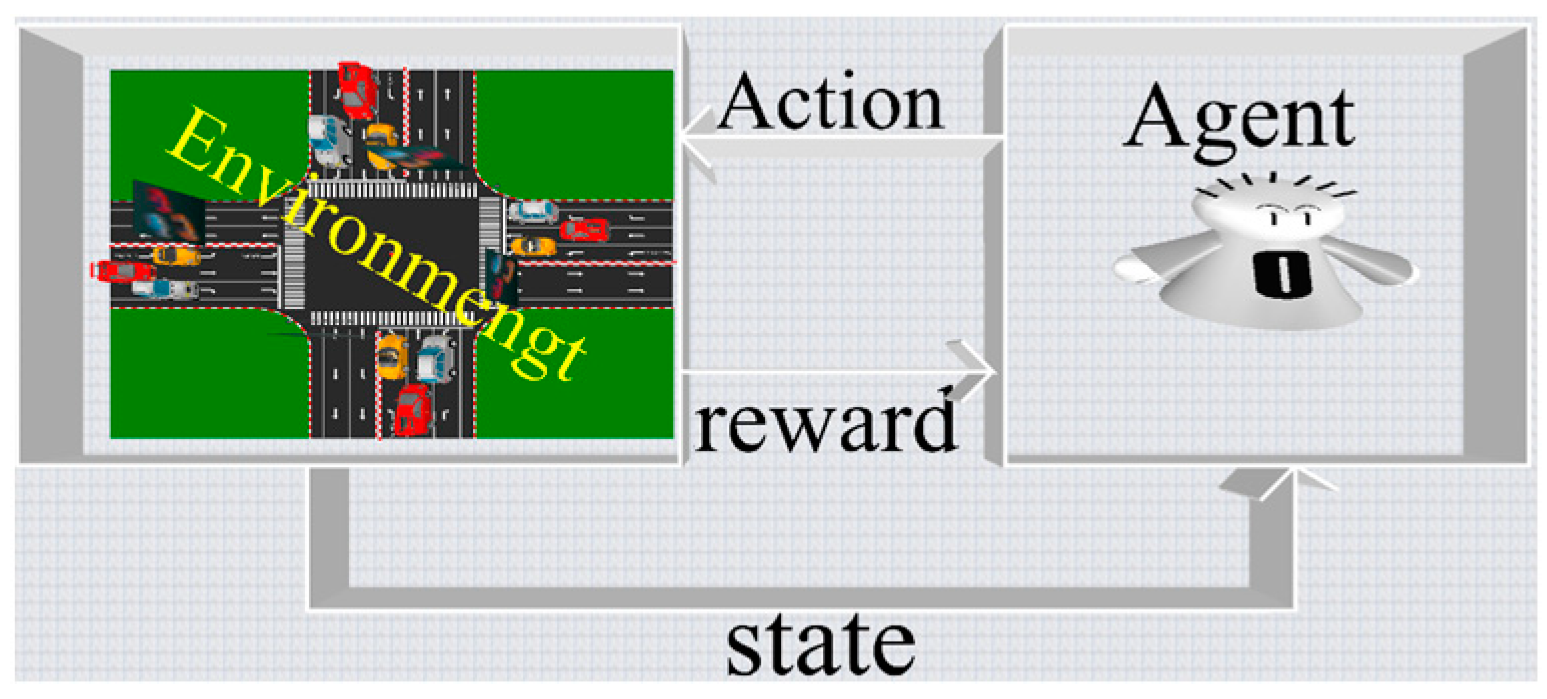
In this study, the intersection signal control problem is formulated as a Markov Decision Process (MDP) [42], where the key components—state space, action space, and reward function—are defined to guide the reinforcement learning process. Reinforcement learning is typically modeled using an MDP, which consists of the following elements:

• A set of states, expressed as $S=\{s_1,s_2,\dots ,s_i\}$;
• A set of actions, expressed as $A=\{a_1,a_2,\dots ,a_n\}$;
• The conversion probability $T\left(s_{t+1}\right|s_t,a_t)$, which indicates the probability that the agent will transition from state $s_t$ to $s_{t+1}$ after taking action $a_t$;
• The reward function $R(s_t,a_t)$, which specifies the reward for taking action $a_t$ in the $s_t$ state. T the goal of reinforcement learning methods is to maximize the cumulative reward, i.e., Equation (1):

  $$R={\sum }_{t=0}^{\infty } {\gamma }^t{r}_{t+1},$$

  (1)

The discount factor $\gamma \in [0,1]$, which reduces the value of future rewards.

The goal of the agent is to determine the optimal strategy to maximize the expected return, which can be determined using the following Equation (2):

$${\pi }^{\ast }=arg \underset{\pi }{max} E[R|\pi ],$$

(2)

The status, actions, and rewards of this article are set as follows.

• State:

In our model, the state at each time step is defined as a combination of the queue length and vehicle speed at each intersection, along with those at neighboring intersections. These two metrics are crucial for assessing traffic congestion and flow. Queue length represents the number of vehicles in each lane and serves as a direct indicator of congestion. Speed reflects the average speed of vehicles in each lane and indicates the smoothness of traffic flow. To obtain this state information, vehicle counts and average speeds are first extracted from the traffic simulation environment. These features are then integrated with the graphical data obtained through the Graph Neural Network (GNN), forming a comprehensive state representation. This representation not only captures the traffic state of individual intersections; it also incorporates the conditions at surrounding intersections, enabling the optimization of the entire traffic network.

Figure 4 provides an example of this state representation. In this figure, each point represents a vehicle in the current lane, with the x-axis showing the vehicle ID, the y-axis indicating its position within the lane (in meters), and the z-axis representing its speed (in meters per second). Different colors are used to denote the travel direction: red for north, blue for south, green for east, and yellow for west. The 3D scatter plot visualizes the distribution of vehicles in the lane and their speeds, showing traffic flow across different directions.

This figure illustrates how our model organizes and processes state data. By tracking vehicle locations and speeds in real time, the system can dynamically adjust traffic signals to improve flow and reduce congestion. The graphical representation also highlights the spatio-temporal relationships between intersections, which is essential for making informed decisions in adaptive traffic signal control. The final state representation example is shown in Figure 4.

• Action:

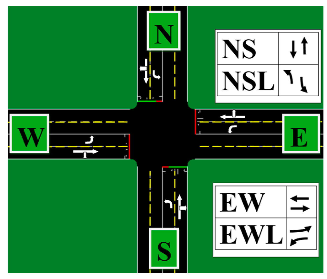
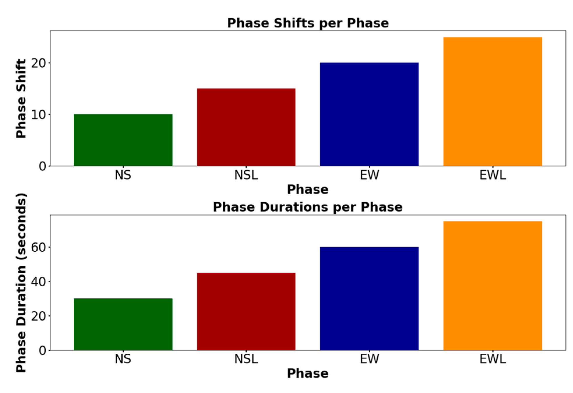
The action space in our model consists of two components: phase shifts and phase durations. Phase Shifts: Represent the change in signal phases, determining which lanes are open for passage at a given time. Phase Durations: Specify how long each phase remains active, controlling the duration of each traffic signal phase. At each time step, the environment updates the state of the traffic light based on a given phase transition and phase duration. An example of the action representation is shown in Figure 5.

• Reward:

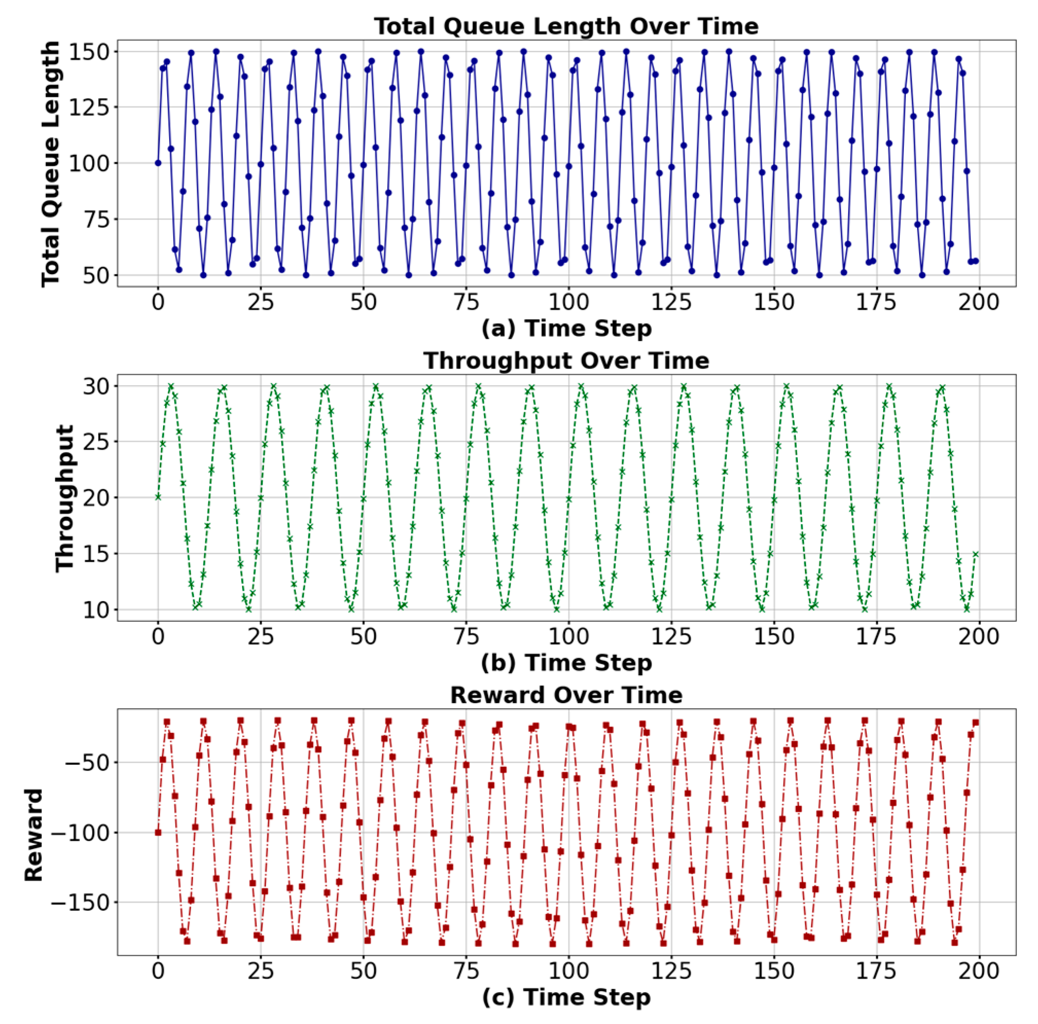
The reward function is designed to balance traffic congestion and traffic smoothness. It consists of two primary components. Negative Queue Length: A penalty that encourages the reduction of vehicles in each lane, aiming to alleviate congestion. An illustration of this penalty is shown in Figure 6a. Throughput: A positive reward that encourages increasing the number of vehicles passing through the intersection, thus improving traffic flow. The throughput reward is shown in Figure 6b. The combined reward is a weighted sum of these two components, with negative rewards for long queues and positive rewards for increased throughput. The overall reward function, combining both aspects, is shown in Figure 6c. By using this reward function, the reinforcement learning agent is incentivized to optimize traffic flow by minimizing congestion while maximizing the throughput of vehicles through the intersection.

Through the above design, this study aims to use GNNs to extract high-dimensional features from complex transportation networks and combine queue length and speed information to form a comprehensive description of traffic status. At the same time, by defining a reasonable action space and reward function, our model can learn an effective traffic signal control strategy to optimize the urban traffic management system.

GNN plays a crucial role in our model. It extracts the complex relationship information between nodes through the convolution operation of the topology and node features of the transportation network. This allows our model to not only account for the local information of individual intersections, but also to capture the global dynamics of the entire transportation network. By combining queue length, velocity, phase conversion, phase duration, and reward functions based on queue length and throughput, our model is able to adaptively optimize signal control strategies in complex urban traffic environments, thereby significantly improving the efficiency of traffic flow and reducing traffic congestion.

For scenarios where the Markov decision process is completely known and its state–action space is limited, we can create a model of the environment in which we interact with the intelligences, called model-based reinforcement learning. However, in real-world TSC, it is challenging to fulfill these conditions, and, therefore, model-free reinforcement learning is more commonly applied in TSC [43]. Model-free reinforcement learning can be further categorized into value-based approaches, policy-based approaches, and combinations of both (AC).

• DESAC algorithm

SAC [44] is an offline policy AC algorithm based on a maximum entropy reinforcement learning framework. Contrary to other RL methods, participants in SAC attempt to maximize entropy while maximizing discounted cumulative rewards. The main idea behind SAC is to combine the off-policy updating from soft Q learning [45] with the AC algorithm. In this way, SAC overcomes the problem of poor sampling efficiency. SAC achieves state-of-the-art performance on RL problems with continuous settings.

Regarding Soft Actor–Critic, SAC learns one policy and two Q-functions at the same time. There are two standard variants of SAC: one uses fixed entropy regularization coefficients, and the other enforces entropy constraints by varying during training. In this paper, we use the DESAC algorithm, which enforces the entropy constraint by varying the entropy regularization coefficients during training, i.e., the DESAC algorithm. The dynamic entropy constraint is a crucial component of our approach designed to balance exploration and exploitation in reinforcement learning. By dynamically adjusting policy randomness, this method enhances the model’s adaptability to different traffic environments. Specifically, in traffic signal control, dynamic entropy constraints enable the model to respond effectively to traffic fluctuations by regulating the probability of signal transitions. For instance, during periods of high traffic flow, the constraint reduces unnecessary signal changes, while in low traffic conditions, it promotes exploration to identify more efficient signal configurations. We implement this mechanism using the DESAC algorithm, which incorporates policy entropy as a guide for exploration. In train_sac, we set a target entropy value (target_entropy) and dynamically adjust the policy’s entropy during training. This dynamic adjustment ensures that the model can adapt its decision-making process to varying traffic conditions, optimizing signal control by reducing congestion during peak periods and enhancing flow during off-peak times. By combining GNN-based feature extraction with DESAC’s dynamic entropy regulation, our method achieves robust and efficient traffic signal control across diverse scenarios.

In the Entropy Regularized Reinforcement Learning (ERRL) setup, the goal is to maximize the weighted sum of the entropy of the reward and the strategy. This setup encourages exploration by increasing the entropy of the strategy so that the strategy is not overly deterministic, leading to better exploration of the state–action space.

• Entropy regularization target;

The goal of entropy regularization can be expressed as optimizing the following objective function:

$$J\left(\pi \right)={\sum }_{t=0}^T {\mathbb{E}}_{(s_t,a_t)\sim {\rho }_{\pi }}\left[r(s_t,a_t)+\alpha \mathcal{H}\left(\pi \right(·\left|s_t\right))\right],$$

(3)

$J\left(\pi \right)$ is the optimization target, ${\rho }_{\pi }$ the distribution of state actions caused by the strategy $\pi$, $r(s_t,a_t)$ is the immediate reward for taking action $a_t$ in state $s_t$, $\mathcal{H}\left(\pi \right(·\left|s_t\right))$ is the entropy of the strategy in state $s_t$, and $\alpha$ is the entropy coefficient, weighing the weight of the immediate reward and the entropy of the strategy.

2.

Definition of entropy;

The goal of entropy regularization can be expressed as optimizing the following objective function:

$$\mathcal{H}\left(\pi \right(·\left|s\right))=-{\sum }_a \pi (a\left|s\right)log \pi \left(a\right|s),$$

(4)

3.

Target Q value calculation;

$$Q_{target}=r+\gamma (1-d)\left(Q(s^{\prime },a^{\prime })-\alpha log \pi \left(a^{\prime }\right|s^{\prime })\right),$$

(5)

$r$ is rewards, $\gamma$ is the discount factor, $d$ is the terminal sign, which indicates whether the termination state has been reached, $Q(s^{\prime },a^{\prime })$ is the Q value of the next state, when $s^{\prime }$ takes action $a^{\prime }$, $\alpha$ is the entropy scale, which controls the randomness of the strategy, and $\mathrm{l}\mathrm{o}\mathrm{g} \pi \left(a^{\prime }\right|s^{\prime })$ is the logarithmic probability of taking action $a^{\prime }$ in state $s^{\prime }$.

4.

Q value updated:

$$L\left(Q\right)={\mathbb{E}}_{(s,a,r,s^{\prime })\sim D}\left[{\displaystyle \frac{1}{2}}{\left(Q(s,a)-Q_{\mathrm{t}\mathrm{a}\mathrm{r}\mathrm{g}\mathrm{e}\mathrm{t}}\right)}^2\right],$$

(6)

$\mathrm{D}$ is the experience replay buffer. $Q_{target}$ is the target Q-value. $Q(s,a)$ is the current Q value. This formula is in the form of the Mean Squared Error (MSE), which represents the loss function of the Q-valued network.

5.

Policy updates:

The goal of the policy update is to minimize the following loss functions:

$$L\left(\pi \right)={\mathbb{E}}_{s\sim D}\left[\alpha log \pi \left(a\right|s)-Q(s,a)\right],$$

(7)

$\mathrm{l}\mathrm{o}\mathrm{g} \pi \left(a\right|s)$ is the logarithmic probability of taking action $a$ in state $s$, and $Q(s,a)$ is the Q value of the action pair in the current state.

6.

Entropy coefficient updated:

The update goal of the entropy coefficient is to minimize the following loss functions:

$$L\left(\alpha \right)=-{\mathbb{E}}_{s\sim D}\left[\alpha \left(log \pi \left(a\right|s)+\mathcal{H}\right)\right],$$

(8)

$\mathcal{H}$ is the target entropy (adjusted for the environment).

7.

The state value function:

In the DESAC algorithm, the state value function $V\left(s\right)$ is indirectly represented by the following relationship:

$$V\left(s\right)=Q(s,a)-\alpha log \pi \left(a\right|s),$$

(9)

This formula is actually embodied in the policy update process. Specifically, the DESAC algorithm uses a soft Q function that combines the value of the action and the logarithmic probability of the strategy, thus being equivalent to the state value function $V\left(s\right)$ to a certain extent.

In the strategy update, the $\alpha \mathrm{l}\mathrm{o}\mathrm{g} \pi \left(a\right|s)$ part of the loss function of Equation (7) can be seen as a manifestation of the state value $V\left(s\right)$, because it adjusts $Q(s,a)$ to take into account both the action value and the entropy of the strategy. Specifically, Equation (7) shows that the state value function $V\left(s\right)$ is expressed indirectly by the action value function $Q(s,a)$ and the entropy of the strategy (i.e., the logarithmic probability of the action). This approach allows the DESAC algorithm to effectively exploit the randomness of the strategy to explore and learn, resulting in better performance. Therefore, although the state value function is not directly defined in the DESAC algorithm, it is indirectly represented by the soft Q function in the policy update.

The state value function $V^{\pi }\left(s\right)$ considering entropy regularization is defined as

$$V^{\pi }\left(s\right)={\mathbb{E}}_{a\sim \pi }\left[Q^{\pi }(s,a)-\alpha log \pi \left(a\right|s)\right],$$

(10)

$V^{\pi }\left(s\right)$ is the value in state $s$, $Q^{\pi }(s,a)$ is the value of the action $a$ taken in state $s$, and $\alpha \mathrm{l}\mathrm{o}\mathrm{g} \pi \left(a\right|s)$ is the entropy term that is used to encourage the randomness of the strategy.

8.

Action value function.

Combined with entropy regularization, the action value function is defined as

$$Q^{\pi }(s,a)=r(s,a)+\gamma {\mathbb{E}}_{s^{\prime }\sim P}\left[\begin{array}{c}{V}^{\pi }\left(s^{\prime }\right)\end{array}\right],$$

(11)

$$Q^{\pi }(s,a)=r(s,a)+\gamma {\mathbb{E}}_{s^{\prime }\sim P}\left[{\mathbb{E}}_{a^{\prime }\sim \pi }\left[Q^{\pi }(s^{\prime },a^{\prime })-\alpha log \pi \left(a^{\prime }\right|s^{\prime })\right]\right],$$

(12)

$r(s,a)$ is the immediate reward, $\gamma$ is the discount factor, and $s^{\prime }$ is the next state.

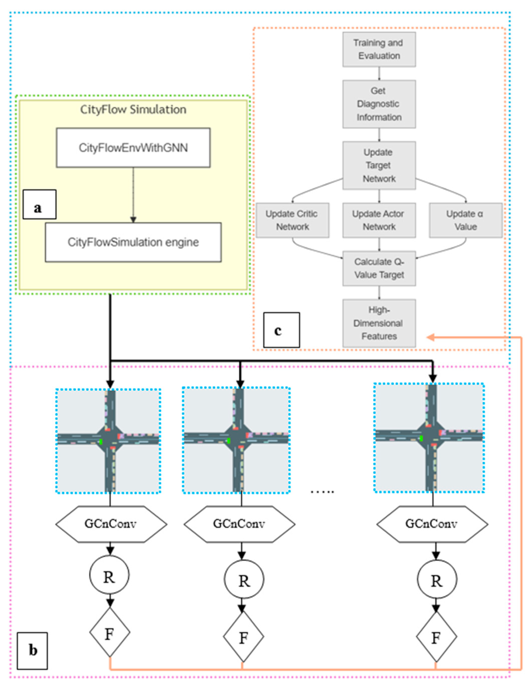
The DESAC algorithm pseudocode is shown in Algorithm 1. The G-DESAC model diagram is shown in Figure 7.

Algorithm 1: DESAC
Input:		Policy network ${\pi }_{\theta }$, two Q networks $Q_{\varphi 1}$, $Q_{\varphi 2}$, target Q networks $targe{t}_{-}{Q}_{\varphi 1}$, $targe{t}_{-}{Q}_{\varphi 2}$, Replay buffer D, entropy coefficient α
Set hyperparameters: discount factor γ, target update coefficient τ, target entropy H;
Initialize α optimizer (for entropy-constrained SAC);
repeat
	Sample an action a from the environment using ${\pi }_{\theta }$ and store ($s,a,r,s^{\prime },d$) in D;
	Sample a batch ($s,a,r,s^{\prime },d$) from D;
	Q-Target Calculation: Sample next action $a^{\prime }\sim {\pi }_{\theta }(a^{\prime }|s^{\prime })$ and log probability $\log {\pi }_{\theta }\left(a^{\prime }|s^{\prime }\right)$;
	Compute
	$Q_{\mathrm{t}\mathrm{a}\mathrm{r}\mathrm{g}\mathrm{e}\mathrm{t}}=r+\gamma (1-d)\left(min(Q_{\varphi 1}(s^{\prime },a^{\prime }),Q_{\varphi 2}(s^{\prime },a^{\prime }))-\alpha \mathrm{l}\mathrm{o}\mathrm{g} {\pi }_{\theta }(a^{\prime }|s^{\prime })\right)$;
	Q-Value Update: Compute current Q-values $Q_{\varphi 1}(s,a)$ and $Q_{\varphi 2}(s,a)$;
	Compute Q loss:
	$L(Q_{\varphi })={\displaystyle \frac{1}{2\left|B\right|}}{\displaystyle \sum _{(s,a,r,s^{\prime },d)\in B}} ((Q_{\varphi }(s,a)-Q_{\mathrm{t}\mathrm{a}\mathrm{r}\mathrm{g}\mathrm{e}\mathrm{t}}{)}^2)$
	Update Q networks $Q_{\varphi 1}$ and $Q_{\varphi 2}$ using gradient descent;
	Policy Update: For each state s in batch, sample action $a\sim {\pi }_{\theta }(a|s)$;
	Compute policy loss:
	$L({\pi }_{\theta })={\displaystyle \frac{1}{\left|B\right|}}{\displaystyle \sum _{s\in B}} \left(\alpha \mathrm{l}\mathrm{o}\mathrm{g} {\pi }_{\theta }(a|s)-min(Q_{\varphi 1}(s,a),Q_{\varphi 2}(s,a))\right)$
	Update policy network ${\pi }_{\theta }$ using gradient ascent;
	Entropy Coefficient Update (for entropy-constrained SAC): Compute entropy loss:
	$L(\alpha )=-{\displaystyle \frac{1}{\left|B\right|}}{\displaystyle \sum _{s\in B}} \alpha \left(\mathrm{l}\mathrm{o}\mathrm{g}{\pi }_{\theta }(a|s)+H\right)$
	Update entropy coefficient α;
	Soft Update of Target Q Networks: Update target Q networks:
	${\varphi }_{\mathrm{t}\mathrm{a}\mathrm{r}\mathrm{g}\mathrm{e}\mathrm{t},i}\leftarrow \tau {\varphi }_i+(1-\tau ){\varphi }_{\mathrm{t}\mathrm{a}\mathrm{r}\mathrm{g}\mathrm{e}\mathrm{t},i} \mathrm{f}\mathrm{o}\mathrm{r} i=1,2$
until;
Return $q\_loss,policy\_loss,alpha\_loss$ (for debugging and monitoring);

3.4. Deep Neural Networks

In the proposed algorithm, three main deep neural network models are involved: GNN-Feature-Extractor, Policy-Network, and Q-Network. They are used for feature extraction, policy generation, and value evaluation, respectively.

1.

GNN-Feature-Extractor;

Input Layer: The connection relationship A between the receiving node feature X and the edge.

The first layer of the graph convolutional layer: the input dimension input-dim is converted to the hidden layer dimension hidden-dim:

$$H^{\left(1\right)}=ReLU\left({AXW}^{\left(0\right)}\right),$$

(13)

where $A$ is the adjacency matrix, $X$ is the input feature matrix, and ${\mathrm{W}}^{\left(0\right)}$ is the weight matrix of the first layer, and the activation function $ReLU$ applies nonlinear activation.

The second layer of the graph convolutional layer converts the hidden layer dimension hidden-dim to the output layer dimension:

$$H^{\left(2\right)}={AH}^{\left(1\right)}{W}^{\left(1\right)},$$

(14)

where $W^{\left(1\right)}$ is the weight matrix of the second layer.

Output Layer: The output graph feature represents $H^{\left(2\right)}$.

GNN-Feature-Extractor is used to extract features from the graph data of the transportation network, capturing the relationship between nodes and edges through graph convolution operations. These characteristics are used as input to subsequent networks (policy networks and Q-networks).

2.

Policy-Network:

Input Layer: Receives the environmental state feature $S$.

The first fully connected layer contains 128 neurons, and the activation function is $\mathrm{R}\mathrm{e}\mathrm{L}\mathrm{U}$.

$$H^{\left(1\right)}=ReLU({SW}^{\left(0\right)}+b^{\left(0\right)}),$$

(15)

where $b^{\left(0\right)}$ is the bias vector of the first fully connected layer.

The second fully connected layer contains 128 neurons and has an activation function of $ReLU$.

$$H^{\left(2\right)}=ReLU(H^{\left(1\right)}{W}^{\left(1\right)}+b^{\left(1\right)}),$$

(16)

where $b^{\left(1\right)}$ is the bias vector of the second fully connected layer.

Output layer: The output is the size of the action space, which represents the probability distribution of each action $\pi$. This layer uses the $Softmax$ function to normalize the output so that the sum of the probabilities of all actions is 1.

$$\pi =Softmax(H^{\left(2\right)}{W}^{\left(2\right)}+b^{\left(2\right)}),$$

(17)

where $Softmax$ is a normalization function that converts multiple values of the output into a probability distribution, and $b^{\left(2\right)}$ is the bias vector of the output layer.

Policy-Network is used to generate action policies. Given the environmental state feature $S$, the network outputs a probability distribution of each possible action $\pi$, and the policy network samples action $\mathrm{a}$ based on this distribution.

3.

Q-Network.

Input layer: Receives the environment state $S$ and the action feature $a$.

The first fully connected layer contains 128 neurons with an activation function of $ReLU$.

$$H^{\left(1\right)}=ReLU({SW}^{\left(0\right)}+b^{\left(0\right)}),$$

(18)

The second fully connected layer contains 128 neurons, and the activation function is $ReLU$.

$$H^{\left(2\right)}=ReLU(H^{\left(1\right)}{W}^{\left(1\right)}+b^{\left(1\right)}),$$

(19)

Output Layer: The output is a single Q value $Q(S,a)$, which represents the value of the state–action pair.

$$Q(S,a)=H^{\left(2\right)}{W}^{\left(2\right)}+b^{\left(2\right)},$$

(20)

Q-Network is used to evaluate the value of state–action pairs. Given the environment state $S$ and the action $a$, the network outputs the corresponding Q value $Q(S,a)$, which is used to estimate the return of taking that action in that state. Together, these deep neural network models form the core components of the algorithm, handling tasks like feature extraction, policy generation, and value evaluation, respectively. The specific process is as follows.

Feature Extraction: Use GNN-Feature-Extractor to extract features of nodes and edges from the graph data of the transportation network. These features capture the relationships between nodes (junctions) and edges (roads) in a transportation network. The formula is as follows:

$$H=\text{GNN-Feature-Extractor}(X,A),$$

(21)

where $H$ is the result of feature extraction, which represents the features of nodes and edges extracted from the transportation network, $X$ represents the node information in the transportation network, and $A$ represents the edge information in the transportation network.

Policy generation: The extracted feature $H$ is passed to Policy-Network as input. The policy network processes the input features and outputs the probability distribution $\pi$ of each possible action. According to the probability distribution, the strategy network samples and selects the optimal action $a$. The formula is as follows:

$$\pi =\text{Policy-Network}\left(H\right),$$

(22)

$$a\sim \pi ,$$

(23)

where $\pi$ represents the output of the policy network and the probability distribution of possible actions and $a$ represents the actions sampled according to the probability distribution $\pi$.

Valuation: The current state and selected actions are passed as input to Q-Network. The Q-network processes the input and outputs the corresponding Q value. The Q value is used to estimate the expected return for taking that action in the current state. The formula is as follows:

$$Q\left(S,a\right)=\text{Q-Network}(S,a),$$

(24)

where $Q(S,a)$ denotes the Q value, the expected return for performing action $a$ in state $S$.

Algorithm training: During the training process, the algorithm continuously uses the above network for feature extraction, policy generation, and value evaluation. Through the deep reinforcement learning method DESAC, the policy network and the Q-network are optimized so that the policy network can choose the actions that can maximize the cumulative return.

4. Experiments and Results

This study presents a simulation experiment to evaluate our proposed method for adaptive traffic signal control, comparing it with currently popular traffic signal control techniques. We begin by describing the selection of the simulation platform and the datasets used in the experiment. This section also provides details about the datasets and their relevance. Next, we outline the comparison methodology, the use of WSL2, the deep learning framework, and the associated libraries. We also explain the setting of model hyperparameters and the performance evaluation metrics. Finally, we report on the experimental results, providing a detailed analysis and drawing conclusions.

For our experiments, we used a newly designed open-source traffic simulator, which is over 20 times faster than SUMO and supports interactive rendering for real-time monitoring. This simulator is capable of handling large-scale traffic signal control, as discussed in [41]. Traffic data are fed into the simulator, where the vehicle travels towards the destination according to the settings of the environment. The simulator then provides states to the signal control system, which performs traffic signal operations based on the input data.

4.1. Datasets

We used real-world traffic flow data for our experiments, which include both two-way dynamic flow and turning flow. The traffic data were sourced from the cities of Hangzhou and Jinan [46,47,48], with road networks imported from OpenStreetMap, as shown in Figure 8.

Table 1. Statistics of the real-world traffic dataset.

Dataset	Intersections	Total Intersections	Total Roads	Arrival Rate (Vehicles/300 s)
				Mean	Std	Max	Min
$D_{Hangzhou}$	1	5	8	185.92	18.65	210	152
$D_{JiNan}$	16	26	62	524.58	98.53	672	256

provides detailed statistics for these datasets. The detailed descriptions on how we preprocessed these datasets are as follows.

$D_{Hangzhou}$: There are 16 intersections in Gudang sub-district, where traffic data come from roadside surveillance cameras. Each record in the dataset includes the time, the camera ID, and vehicle information. By analyzing these records with camera locations, the trajectories of vehicles passing through the intersections can be recorded. We experimented by selecting the number of vehicles at an intersection with the largest Referred result [10] as the traffic flow.

$D_{JiNan}$: Similarly to $D_{Hangzhou}$, these traffic data are collected by roadside cameras near 12 intersections in Dongfeng Sub-district, Jinan, China.

Our focus in this study is on optimizing traffic signal control. Upon analyzing the real-world traffic data, we found that the distribution of vehicle arrival times closely follows the Weibull distribution, as illustrated in Figure 9a,b. This observation not only confirms the statistical properties of the data but also serves as a crucial foundation for designing signal control strategies. The shape and scale parameters of the Weibull distribution allow us to simulate arrival patterns under different traffic conditions and thus fine-tune signal control.

4.2. Comparative Methods and Evaluation Indicators

4.2.1. Comparative Methods

In this study, we compare our proposed method with several widely used traffic signal control algorithms. To ensure a fair comparison, all algorithms are executed under identical environment settings, hyperparameters, and training conditions. A unified evaluation metric is used across all methods, and the results are averaged over multiple experiments to ensure reliability and consistency.

1.

DQN (Deep Q-Network)

DQN is an algorithm that integrates deep learning with Q-learning. It uses a deep neural network to approximate the Q-function. In the context of traffic signal control, DQN learns optimal signal control strategies based on real-time traffic data, such as vehicle count and wait times. DQN stabilizes the learning process through continuous interaction with the environment, experience replay, and target networks.

2.

DDPG (Deep Deterministic Policy Gradient)

DDPG is a reinforcement learning algorithm designed for continuous action spaces, combining ideas from policy gradient methods and Q-learning. For traffic signal control, DDPG fine-tunes signal durations to optimize traffic flow. The algorithm uses an actor-critic framework, along with experience replay and target networks, to improve learning efficiency and stability.

3.

Max-Pressure Control

Max-Pressure Control is a rule-based approach to traffic signal control that aims to maximize the outflow rate at intersections. This method calculates the pressure at each phase—defined as the difference between the number of vehicles in the inlet and exit lanes—and uses this value to determine when to switch signals. While simple and easy to implement, Max-Pressure Control may not adapt well to dynamic traffic conditions.

4.

SAC (Soft Actor–Critic)

SAC is a deep reinforcement learning algorithm that incorporates stochastic strategies and entropy regularization. It uses two networks, a policy network and a value network, while considering the entropy of the policy to promote exploration. SAC performs well in continuous action spaces, making it particularly suited to traffic signal control tasks that require a balance between exploration and exploitation.

The model is trained iteratively using the CityFlow simulation environment, which is developed for Unix-based systems. For this study, we ran WSL2 on Windows 11 and created a virtual environment (myenv) on Ubuntu 22.04.5 LTS to debug and execute the code. The reinforcement learning environment is provided by the Gym library, and the deep learning framework uses PyTorch and TensorFlow. The experiment runs on Python 3.10. The hyperparameters for each method are summarized in

Table 2. Hyperparameters.

Hyperparameter	Single Intersection	Multiple Intersections
Number of iterations	650	1000
Number of training steps per round steps	6500	5000
Batch size	512	256
Sampler max path length	1000	1000
Pool max size R	100,000	100,000
Discount Factor γ	0.99	0.99
Tau	0.005	0.005
Reward scale	1	0.1
Policy Learning Rate	1 × 10−6	1 × 10−6
Q Learning Rate	1 × 10−6	1 × 10−6
Alpha Learning Rate	1 × 10−6	1 × 10−6
Target update interval	1	1

.

A sensitivity analysis was conducted on key hyperparameters, including the learning rate and Tau, to evaluate the model’s performance robustness. The results of this analysis are illustrated in Figure 10a,b.

4.2.2. Evaluation Metrics

In this study, three key metrics are used to evaluate the effectiveness of the traffic signal optimization methods: delay time, queue length, and throughput.

Delay time measures the amount of time vehicles spend waiting at an intersection, which impacts both driving experience and fuel consumption.

Queue length reflects the degree of traffic congestion at an intersection and is crucial for optimizing signal control.

Throughput indicates the number of vehicles that can pass through an intersection in a given time period, serving as a critical indicator of the effectiveness of traffic signal optimization strategies.

4.3. Experimental Results and Discussion

This subsection presents the results of the traffic flow simulations and provides a comprehensive quantitative comparison with other methods. Figure 11 and Figure 12 display the total reward and performance metrics—total delay time, total queue length, and throughput—for all methods over the course of the simulation.

• Total Reward:

We set the total reward to a combination of negative queue length and throughput, with the throughput weighted at 10. This reward structure is designed to optimize overall system performance by encouraging the algorithms to balance congestion reduction with processing efficiency. The simulation results are shown in Figure 11a and Figure 12a.

Figure 11a shows the total reward evolution of five algorithms across different training rounds in a single-intersection scenario. G-DESAC demonstrates clear superiority, with a steady increase in reward after initial fluctuations, particularly after 600 rounds, where its performance surpasses all other algorithms. This reflects G-DESAC’s strong learning ability and optimization effectiveness. In contrast, DQN shows good early performance but experiences significant fluctuations and a downward trend later in the training. SAC (purple line) remains relatively stable around a reward value of 1000, without much improvement. Max-Pressure Control exhibits the largest reward fluctuations, indicating instability and weaker overall performance. DDPG shows little variation, suggesting that it may be stuck in a local optimum and unable to explore adequately or further optimize the strategy. In summary, G-DESAC not only outperforms the other algorithms in the later stages but also shows better stability and consistent improvement, demonstrating the best traffic signal control performance in the single-intersection scenario.

Figure 12a shows the total reward trends for the five algorithms in a multi-intersection scenario. G-DESAC and SAC both perform well, maintaining high reward levels and smooth training progress. However, G-DESAC slightly outperforms SAC, showing a higher and less fluctuating reward trajectory, indicating more stable and efficient optimization of the traffic signal control strategy. In contrast, Max-Pressure and DQN show increasing rewards but with larger fluctuations, resulting in less stability. DDPG, similarly to the single-intersection case, fails to learn effectively and shows a flat reward curve.

Overall, G-DESAC outperforms all other methods both in single intersection and multi-intersection scenarios. It combines the advantages of SAC with improved stability and more consistent optimization, making it the most effective approach for traffic signal control in both simple and complex environments.

• Total delay time and total queue length and throughput:

As shown in Figure 11b–d, the G-DESAC model consistently outperforms other algorithms in terms of total delay time, queue length, and throughput in single intersection traffic control. Total delay time: G-DESAC significantly reduces vehicle waiting times, achieving the best control effect in this metric. Queue length: The algorithm maintains the lowest queue length, successfully preventing traffic congestion. Throughput: G-DESAC improves the throughput rate at the intersection, optimizing the flow of traffic. Although the total latency and queue length of G-DESAC were slightly higher than SAC after 600 rounds of training, they were again lower than SAC around 650 rounds. In addition, G-DESAC demonstrates high stability, with minimal fluctuations during training, maintaining consistent performance as training progresses. In contrast, algorithms like Max-Pressure, DQN, DDPG, and SAC exhibit relatively poor performance, particularly in delay time and throughput control. These results suggest that G-DESAC has significant potential for real-world traffic signal control applications.

In Figure 12b–d, the G-DESAC model also excels in multi-intersection scenarios, outperforming other algorithms in terms of total delay time, total queue length, and throughput at twelve intersections. Total delay time: G-DESAC maintains a delay time of around 200 with minimal fluctuations, demonstrating its stability and efficiency in optimizing traffic signal control. Queue length: The algorithm keeps the queue length low, effectively reducing vehicle waiting times. Throughput: G-DESAC maintains a throughput of around 150 with small fluctuations, ensuring high vehicle throughput efficiency. In contrast, DDPG exhibits extreme performance issues in terms of delay and queue length. Its flat reward curve suggests the algorithm may have become stuck in local optima with insufficient exploration during training, leading to poor optimization. Additionally, DDPG shows low throughput, making it less practical for real-world applications. DQN and Max-Pressure algorithms also show higher fluctuations and instability, while SAC, despite achieving the highest throughput, struggles with higher delay times and queue lengths, which could potentially cause traffic congestion.

Overall, G-DESAC excels in stability, efficiency, and overall performance, making it the ideal choice for practical traffic signal control in both single-intersection and multi-intersection scenarios.

In order to quantitatively show the advantages of the proposed method over alternative methods,

Table 3. Average indicators of each algorithm at a single intersection.

	Delay	Queue Length	Throughput
DESAC_GNN	14.563077	32.344615	18.033846
DDPG	5.721538	21.950769	16.278462
DQN	122.452308	131.164615	8.806154
MAX Pressure	173.363077	179.598462	6.310769
SAC	18.926154	34.226154	15.310769

and

Table 4. Average indexes of each algorithm at the 12 intersections.

	Delay	Queue Length	Throughput
DESAC_GNN	239.148	428.966	193.546
DDPG	99.000	216.000	117.000
DQN	453.526	580.822	128.016
MAX Pressure	406.220	530.369	124.888
SAC	289.120	510.486	224.877

summarize the average metrics for each algorithm. In addition, the relative percentage differences in performance indicators between the deep reinforcement learning method and other methods in this paper are shown in

Table 5. Relative percentage difference of single intersection (based on DESAC_GNN).

	DDPG	DQN	MAX Pressure	SAC
Delay	−60.71	740.84	1090.43	29.96
Queue length	−32.13	305.52	455.27	5.82
Throughput	−9.73	−51.17	−65.01	−15.1

and

Table 6. Relative percentage difference of 12 intersections (based on DESAC_GNN).

	DDPG	DQN	MAX Pressure	SAC
Delay	−58.6	89.64	69.86	20.9
Queue length	−49.65	35.4	23.64	19.0
Throughput	−39.55	−33.86	−35.47	16.19

. A negative value indicates that the alternative method is lower than G-DESAC on the “throughput” metric, while a positive value indicates that the alternative method is performing poorly (higher latency and queue length) for the “delay” and “queue length” metrics. At the same time, the calculation results of the relative percentage difference (based on G-DESAC) are displayed in the form of a graph to facilitate visual comparison, as shown in Figure 13 of the relative percentage difference of the single intersection and Figure 14 of the relative percentage difference of the twelfth intersection.

G-DESAC does exceptionally well in both single and twelve intersection scenarios, according to the average index data in Table 3 and Table 4. With a throughput of 18.033846 and a low delay time and queue length of 14.563077 and 32.344615, respectively, G-DESAC surpasses other algorithms in the single intersection case. SAC comes in second. In particular, DDPG has lower latency and queue lengths because it fails to further optimize the strategy during training due to local optimization and inadequate exploration, and its throughput is only 16.278462, which is marginally worse than G-DESAC. In terms of latency and throughput, DQN and MAX Pressure perform noticeably worse than DQN. In particular, MAX Pressure’s latency can reach 173.363077, while DQN’s throughput is only 8.806154.

In the case of the 12th intersection, the G-DESAC performs equally well. The latency is 239.148, the queue length is 428.966, and the throughput is 193.546. Although the throughput is lower than that of SAC, its comprehensive performance far exceeds that of DDPG, DQN, MAX Pressure, and SAC algorithms. In particular, DQN has a latency of 453.526 s, and MAX Pressure has a queue length of 597.842. In the same way, DDPG has the same reason for lower latency and queue length.

Based on the relative percentage differences in Table 5 and Table 6, G-DESAC significantly outperforms the alternative algorithm on several key performance indicators. In the single intersection scenario, the delay and queuing length of DDPG are lower than those of G-DESAC, because DDPG falls into local optimization and insufficient exploration in the training process and fails to further optimize the strategy, and its throughput is 9.73% lower. DQN has a 740.84% higher latency, a 305.52% increase in queue length, and a 51.17% decrease in throughput. MAX Pressure and SAC are also significantly inferior to G-DESAC in latency and queue length, especially MAX Pressure’s latency, which increased by 1090.43%, and throughput decreased by 65.01%.

In the 12 intersection scenario, the relative advantage of G-DESAC is still obvious, and DQN, MAX Pressure, and SAC are also significantly inferior to G-DESAC in terms of latency. DDPG still fell into local optimization and insufficient exploration during the training process, it failed to further optimize the strategy, and its throughput decreased by 39.55%. DQN’s queue length increased by 35.4% and throughput decreased by 33.86%. MAX Pressure increased the queue length by 23.64% and the throughput decreased by 35.47%. SAC increased the queue length by 19.0% and throughput by 16.19%.

In summary, the DDPG algorithm, while achieving low delay and queue lengths, converges too early to a local optimum. As a result, its strategy fails to sufficiently explore better solutions, leading to near-constant values for reward, total delay, queue length, and throughput, which indicates inefficient learning during training. On the other hand, while SAC achieves the highest throughput in multi-intersection scenarios, it suffers from high delay and queue length, which can lead to traffic congestion. In contrast, the G-DESAC model excels in both single intersection and complex multi-intersection scenarios. It effectively reduces delay and queue length while maintaining high throughput, making it more suitable for challenging traffic signal control situations.

The G-DESAC model’s superior performance in multi-intersection scenarios is largely attributed to the unique capabilities of Graph Neural Networks (GNNs) in handling spatial distributional characteristics. GNNs can capture and learn the dependencies and interactions between multiple intersections, which is critical for traffic signal optimization. By representing a road network as a graph, where nodes correspond to intersections and edges represent road connections, GNNs use a message-passing mechanism to share and update information across the network [49]. This enables each intersection to consider both its own state and the traffic conditions of neighboring intersections, facilitating the formulation of a more optimal traffic signal control strategy.

In practical applications, although G-DESAC demonstrates strong performance in simulation environments, real-world deployment requires careful consideration of computational resource demands. The model’s computational complexity arises primarily from the message-passing process in the GNN and the updating of the reinforcement learning strategy. While current computing infrastructure, particularly GPU-equipped servers, can support real-time applications of the G-DESAC model, real-world deployments must also account for data transfer latency and model inference time. Preliminary evaluations suggest that using edge computing devices or cloud platforms can mitigate these delays and enable real-time traffic signal control. Further testing is needed to assess the scalability and adaptability of the model in diverse transportation environments.

5. Conclusions

This paper proposes a novel deep reinforcement learning method for adaptive traffic signal control called G-DESAC (Graph Neural Network and Dynamic Entropy-Constrained Soft Actor–Critic). The method is validated within the CityFlow simulation environment and is capable of capturing both global and local features of the road network. This enables the model to provide more comprehensive traffic information for decision making and dynamically adjust the signal control strategy based on real-time traffic conditions with high adaptability. Experimental results demonstrate that G-DESAC performs exceptionally well in both single intersection and more complex twelve intersection scenarios, maintaining stable performance across various traffic conditions. The model effectively reduces delays and queue length while maintaining high throughput.

However, the approach has some limitations. The training and execution of the algorithms demand significant computational resources, which may pose challenges for real-time deployment. Additionally, the system’s complexity, involving the coordination of multiple modules, increases the difficulty of debugging and maintenance. Furthermore, the method relies on high-quality, accurate traffic data, and any missing or erroneous data could negatively impact the model’s performance.

Looking ahead, we aim to optimize the model to reduce computational resource consumption and enhance operational efficiency. We will explore data augmentation techniques to improve the model’s adaptability to a wider range of traffic scenarios and consider incorporating multi-task learning approaches to enhance its generalization and robustness. Future work will include testing the model in diverse urban environments to assess its adaptability and robustness across different geographic and socioeconomic contexts. Incorporating real-time traffic incident data is another key direction, as this could significantly improve the responsiveness and effectiveness of traffic signal control, leading to more efficient and safer urban traffic management.

Additionally, we will investigate solutions for low-data or resource-constrained environments, focusing on techniques for handling sparse or noisy traffic data and optimizing algorithms for devices with limited computational capacity. The broader societal impact of adaptive traffic signal control systems is also an important consideration. Our approach could contribute to key transportation goals, such as reducing emissions and enhancing public safety, thereby offering significant benefits for urban sustainability and the overall quality of life for city residents.

References

1. Mnih, V.; Kavukcuoglu, K.; Silver, D.; Rusu, A.A.; Veness, J.; Bellemare, M.G.; Graves, A.; Riedmiller, M.; Fidjeland, A.K.; Ostrovski, G. Human-level control through deep reinforcement learning. Nature 2015, 518, 529–533. [Google Scholar] [CrossRef] [PubMed]
2. Zhou, M.; Qu, X.; Li, X. A recurrent neural network based microscopic car following model to predict traffic oscillation. Transp. Res. Part C Emerg. Technol. 2017, 84, 245–264. [Google Scholar] [CrossRef]
3. Van der Pol, E.; Oliehoek, F.A. Coordinated deep reinforcement learners for traffic light control. In Proceedings of the Learning, Inference and Control of Multi-Agent Systems (at NIPS 2016), Barcelona, Spain, 9 December 2016; pp. 21–38. [Google Scholar]
4. El-Tantawy, S.; Abdulhai, B. An agent-based learning towards decentralized and coordinated traffic signal control. In Proceedings of the 13th International IEEE Conference on Intelligent Transportation Systems, Funchal, Portugal, 19–20 September 2010; pp. 665–670. [Google Scholar]
5. Zhou, M.; Yu, Y.; Qu, X. Development of an efficient driving strategy for connected and automated vehicles at signalized intersections: A reinforcement learning approach. IEEE Trans. Intell. Transp. Syst. 2019, 21, 433–443. [Google Scholar] [CrossRef]
6. Tsuboi, T.; Mizutani, T. Traffic Congestion “Gap” Analysis in India. In Proceedings of the 7th International Conference on Vehicle Technology and Intelligent Transport Systems, Online Streaming, 28–30 April 2021. [Google Scholar]
7. Yue, W.; Li, C.; Mao, G.; Cheng, N.; Zhou, D. Evolution of road traffic congestion control: A survey from perspective of sensing, communication, and computation. China Commun. 2021, 18, 151–177. [Google Scholar] [CrossRef]
8. Yue, W.; Li, C.; Chen, Y.; Duan, P.; Mao, G. What Is the Root Cause of Congestion in Urban Traffic Networks: Road Infrastructure or Signal Control? IEEE Trans. Intell. Transp. Syst. 2021, 3, 8662–8679. [Google Scholar] [CrossRef]
9. Luk, J. Two traffic-responsive area traffic control methods: SCAT and SCOOT. Traffic Eng. Control 1984, 25, 14. [Google Scholar]
10. Cools, S.-B.; Gershenson, C.; D’Hooghe, B. Self-organizing traffic lights: A realistic simulation. In Self-Organization: Applied Multi-Agent Systems; Springer: Berlin/Heidelberg, Germany, 2013; pp. 45–55. [Google Scholar] [CrossRef]
11. LeCun, Y.; Bengio, Y.; Hinton, G. Deep learning. Nature 2015, 521, 436–444. [Google Scholar] [CrossRef]
12. Haydari, A.; Yılmaz, Y. Deep reinforcement learning for intelligent transportation systems: A survey. IEEE Trans. Intell. Transp. Syst. 2020, 23, 11–32. [Google Scholar] [CrossRef]
13. Schmidhuber, J. Deep learning in neural networks: An overview. Neural Netw. 2015, 61, 85–117. [Google Scholar] [CrossRef]
14. Zurada, J. Introduction to Artificial Neural Systems; West Publishing Co.: Eagan, MN, USA, 1992. [Google Scholar]
15. He, K.; Zhang, X.; Ren, S.; Sun, J. Deep residual learning for image recognition. In Proceedings of the IEEE Conference on Computer Vision and Pattern Recognition, Las Vegas, NV, USA, 27–30 June 2016; pp. 770–778. [Google Scholar]
16. Kenton, J.D.M.-W.C.; Toutanova, L.K. Bert: Pre-training of deep bidirectional transformers for language understanding. In Proceedings of the naacL-HLT, Minneapolis, MN, USA, 2–7 June 2019; p. 2. [Google Scholar]
17. Yadav, P.; Mishra, A.; Kim, S. A comprehensive survey on multi-agent reinforcement learning for connected and automated vehicles. Sensors 2023, 23, 4710. [Google Scholar] [CrossRef]
18. Mnih, V. Playing atari with deep reinforcement learning. arXiv 2013, arXiv:1312.5602. [Google Scholar]
19. Li, D.; Wu, J.; Xu, M.; Wang, Z.; Hu, K. Adaptive traffic signal control model on intersections based on deep reinforcement learning. J. Adv. Transp. 2020, 2020, 6505893. [Google Scholar] [CrossRef]
20. Xie, J.; Yang, Z.; Lai, X.; Liu, Y.; Yang, X.B.; Teng, T.-H.; Tham, C.-K. Deep reinforcement learning for dynamic incident-responsive traffic information dissemination. Transp. Res. Part E Logist. Transp. Rev. 2022, 166, 102871. [Google Scholar] [CrossRef]
21. Cai, C.; Wei, M. Adaptive urban traffic signal control based on enhanced deep reinforcement learning. Sci. Rep. 2024, 14, 14116. [Google Scholar] [CrossRef]
22. Zeinaly, Z.; Sojoodi, M.; Bolouki, S. A resilient intelligent traffic signal control scheme for accident scenario at intersections via deep reinforcement learning. Sustainability 2023, 15, 1329. [Google Scholar] [CrossRef]
23. Wang, Z.; Yang, K.; Li, L.; Lu, Y.; Tao, Y. Traffic signal priority control based on shared experience multi-agent deep reinforcement learning. IET Intell. Transp. Syst. 2023, 17, 1363–1379. [Google Scholar] [CrossRef]
24. Jung, J.; Kim, I.; Yoon, J. EcoMRL: Deep reinforcement learning-based traffic signal control for urban air quality. Int. J. Sustain. Transp. 2024, 1–10. [Google Scholar] [CrossRef]
25. Chang, A.; Ji, Y.; Wang, C.; Bie, Y. CVDMARL: A Communication-Enhanced Value Decomposition Multi-Agent Reinforcement Learning Traffic Signal Control Method. Sustainability 2024, 16, 2160. [Google Scholar] [CrossRef]
26. Deng, F.; Jin, J.; Shen, Y.; Du, Y. A dynamic self-improving ramp metering algorithm based on multi-agent deep reinforcement learning. Transp. Lett. 2024, 16, 649–657. [Google Scholar] [CrossRef]
27. Xu, M.; Wu, J.; Huang, L.; Zhou, R.; Wang, T.; Hu, D. Network-wide traffic signal control based on the discovery of critical nodes and deep reinforcement learning. J. Intell. Transp. Syst. 2020, 24, 1–10. [Google Scholar] [CrossRef]
28. Zhao, Z.; Wang, K.; Wang, Y.; Liang, X. Enhancing traffic signal control with composite deep intelligence. Expert Syst. Appl. 2024, 244, 123020. [Google Scholar] [CrossRef]
29. Mao, F.; Li, Z.; Li, L. A comparison of deep reinforcement learning models for isolated traffic signal control. IEEE Intell. Transp. Syst. Mag. 2022, 15, 160–180. [Google Scholar] [CrossRef]
30. Fuad, M.R.T.; Fernandez, E.O.; Mukhlish, F.; Putri, A.; Sutarto, H.Y.; Hidayat, Y.A.; Joelianto, E. Adaptive deep q-network algorithm with exponential reward mechanism for traffic control in urban intersection networks. Sustainability 2022, 14, 14590. [Google Scholar] [CrossRef]
31. Zai, W.; Yang, D. Improved deep reinforcement learning for intelligent traffic signal control using ECA_LSTM network. Sustainability 2023, 15, 13668. [Google Scholar] [CrossRef]
32. Zhang, X.; He, Z.; Zhu, Y.; You, L. DRL-based adaptive signal control for bus priority service under connected vehicle environment. Transp. B Transp. Dyn. 2023, 11, 1455–1477. [Google Scholar] [CrossRef]
33. Lee, E.H.; Lee, E. Congestion boundary approach for phase transitions in traffic flow. Transp. B Transp. Dyn. 2024, 12, 2379377. [Google Scholar] [CrossRef]
34. Hollbeck, G.B.; Wang, S.; Schreckenberg, M.; Guhr, T.; Dawson, K.A.; Indekeu, J.O.; Stanley, H.E.; Tsallis, C. Congestions and spectral transitions in time-lagged correlations of motorway traffic. Phys. A Stat. Mech. Appl. 2024, 649, 129952. [Google Scholar] [CrossRef]
35. Drliciak, M.; Cingel, M.; Celko, J.; Panikova, Z. Research on Vehicle Congestion Group Identification for Evaluation of Traffic Flow Parameters. Sustainability 2024, 16, 1861. [Google Scholar] [CrossRef]
36. Laval, J.A. Traffic Flow as a Simple Fluid: Toward a Scaling Theory of Urban Congestion. Transp. Res. Rec. 2024, 2678, 376–386. [Google Scholar] [CrossRef]
37. Messmer, A.; Papageorgiou, M. METANET: A macroscopic simulation program for motorway networks. Traffic Eng. Control 1990, 31, 466–470. [Google Scholar]
38. Barceló, J.; Casas, J. Dynamic network simulation with AIMSUN. In Simulation Approaches in Transportation Analysis: Recent Advances and Challenges; Springer: Berlin/Heidelberg, Germany, 2005; pp. 57–98. [Google Scholar]
39. Manual, G. Virginia Department of Transportation. 1983. Available online: http://166.67.201.35/projects/resources/noisewalls/Highway_Traffic_Noise_Guidance_Manual_V9_acc021822.pdf (accessed on 2 December 2024).
40. Lopez, P.A.; Behrisch, M.; Bieker-Walz, L.; Erdmann, J.; Flötteröd, Y.-P.; Hilbrich, R.; Lücken, L.; Rummel, J.; Wagner, P.; Wießner, E. Microscopic traffic simulation using sumo. In Proceedings of the 2018 21st International Conference on Intelligent Transportation Systems (ITSC), Maui, HI, USA, 4–7 November 2018; pp. 2575–2582. [Google Scholar]
41. Zhang, H.; Feng, S.; Liu, C.; Ding, Y.; Zhu, Y.; Zhou, Z.; Zhang, W.; Yu, Y.; Jin, H.; Li, Z. Cityflow: A multi-agent reinforcement learning environment for large scale city traffic scenario. In Proceedings of the World Wide Web Conference, San Francisco, CA, USA, 13–17 May 2019; pp. 3620–3624. [Google Scholar]
42. Bellman, R. A Markovian decision process. J. Math. Mech. 1957, 6, 679–684. [Google Scholar] [CrossRef]
43. Zhao, H.; Dong, C.; Cao, J.; Chen, Q. A survey on deep reinforcement learning approaches for traffic signal control. Eng. Appl. Artif. Intell. 2024, 133, 108100. [Google Scholar] [CrossRef]
44. Haarnoja, T.; Zhou, A.; Abbeel, P.; Levine, S. Soft actor-critic: Off-policy maximum entropy deep reinforcement learning with a stochastic actor. In Proceedings of the International Conference on Machine Learning, Stockholm, Sweden, 15 July 2018; pp. 1861–1870. [Google Scholar]
45. Haarnoja, T.; Tang, H.; Abbeel, P.; Levine, S. Reinforcement learning with deep energy-based policies. In Proceedings of the International Conference on Machine Learning, Sydney, Australia, 6–11 August 2017; pp. 1352–1361. [Google Scholar]
46. Wei, H.; Zheng, G.; Gayah, V.; Li, Z. A survey on traffic signal control methods. arXiv 2019, arXiv:1904.08117. [Google Scholar]
47. Wei, H.; Xu, N.; Zhang, H.; Zheng, G.; Zang, X.; Chen, C.; Zhang, W.; Zhu, Y.; Xu, K.; Li, Z. Colight: Learning network-level cooperation for traffic signal control. In Proceedings of the 28th ACM International Conference on Information and Knowledge Management, Beijing China, 3–7 November 2019. [Google Scholar]
48. Zheng, G.; Xiong, Y.; Zang, X.; Feng, J.; Wei, H.; Zhang, H.; Li, Y.; Xu, K.; Li, Z. Learning phase competition for traffic signal control. In Proceedings of the 28th ACM International Conference on Information and Knowledge Management, Beijing, China, 3–7 November 2019; pp. 1963–1972. [Google Scholar]
49. Wu, Z.; Pan, S.; Chen, F.; Long, G.; Zhang, C.; Yu, P.S. A Comprehensive Survey on Graph Neural Networks. IEEE Trans. Neural Netw. Learn. Syst. 2021, 32, 4–24. [Google Scholar] [CrossRef] [PubMed]
Figure 1. Basic framework of reinforcement learning.
Electronics 13 04794 g001
Figure 2. Transportation network diagram.
Electronics 13 04794 g002
Figure 3. Algorithm framework diagram. (a) Environment Simulation Module, (b) GNN Feature Extraction Module, (c) Reinforcement Learning Module.
Electronics 13 04794 g003
Figure 4. State diagram.
Electronics 13 04794 g004
Figure 5. Action diagram.
Electronics 13 04794 g005
Figure 6. Reward diagram.
Electronics 13 04794 g006
Figure 7. DESAC-GNN model diagram. The red circle indicates the current location of the inserted experience, indicating where the next experience will be stored.
Electronics 13 04794 g007
Figure 8. Real-world intersection diagram. The colored lines are the enclosed areas, and the green dots are the marked intersections.
Electronics 13 04794 g008
Figure 9. The trend of the number of vehicles in the simulation step.
Electronics 13 04794 g009
Figure 10. Hyperparametric sensitivity analysis.
Electronics 13 04794 g010
Figure 11. Single intersection.
Electronics 13 04794 g011aElectronics 13 04794 g011b
Figure 12. Twelve intersections.
Electronics 13 04794 g012aElectronics 13 04794 g012b
Figure 13. Relative percentage difference analysis at a single intersection: (a) delay, (b) queue length, and (c) throughput.
Electronics 13 04794 g013
Figure 14. Relative percentage difference analysis across 12 intersections: (a) delay, (b) queue length, and (c) throughput.
Electronics 13 04794 g014