Abstract
In complex marine environments, autonomous underwater vehicles (AUVs) rely on robust navigation and positioning. Traditional algorithms face challenges from sensor outliers and non-Gaussian noise, leading to significant prediction errors and filter divergence. Outliers in sensor observations also impact positioning accuracy. The original unscented Kalman filter (UKF) based on the minimum mean square error (MMSE) criterion suffers from performance degradation under these conditions. This paper enhances the minimum error entropy unscented Kalman filter algorithm using variational Bayesian (VB) methods and mixed entropy functions. By implementing minimum error entropy (MEE) and mixed kernel functions in the UKF, the algorithm’s robustness under complex underwater conditions is improved. The VB method adaptively fits the measurement noise covariance, enhancing adaptability to marine environments. Simulations and sea trials validate the proposed algorithm’s performance, showing significant improvements in navigation accuracy and root mean square error (RMSE). In environments with complex noise, our algorithm improves the overall navigation accuracy by at least 10% over other existing algorithms. This demonstrates the high accuracy and robustness of the algorithm.
1. Introduction
As a highly autonomous and controllable underwater exploration tool, AUVs are widely used in military applications, hydrographic surveys, marine environmental monitoring, and mining exploration. Ensuring the proper functioning of the navigation system is a prerequisite for the normal operation of AUVs and is a critical task. Accurate underwater positioning and navigation are fundamental for AUVs to complete complex tasks, as they are crucial for effective data collection and the safe execution of missions.
In the absence of buildings and water barriers, most outdoor robots and aerial robots can use a global positioning system (GPS) for positioning and navigation. However, in underwater environments, GPS signals rapidly attenuate with an increase in AUV working depth, making GPS unusable. Additionally, the complex and variable marine environment poses challenges for the accurate underwater positioning and navigation of AUVs.
Currently, there are many methods specifically applied to underwater navigation in the industry. These methods can generally be categorized into two groups based on the source of navigation information: internal navigation and external navigation [1]. External navigation mainly includes acoustic navigation and geophysical navigation. Most acoustic transponders, such as short baseline (SBL), ultra-short baseline (USBL), long baseline (LBL), and various sonar devices can only operate AUVs within the limited areas constrained by the acoustic equipment. These devices are difficult to deploy and maintain on the seabed, greatly limiting their use. Geophysical navigation relies on prior environmental knowledge to map positions, but due to the absence of pre-existing marine environment maps and the significant expenses involved, this method is challenging to apply widely. Internal navigation techniques primarily encompass simultaneous localization and mapping (SLAM) as well as inertial or dead reckoning. These approaches provide a more adaptable solution but also come with their own set of challenges and limitations [2,3]. The SLAM algorithm is booming in the field of navigation and positioning in unknown environments [4]. Based on the SLAM method, AUVs can simultaneously construct environmental maps and localize themselves within these maps. Sonar is typically used for underwater SLAM, but the high expense of sonar sensors makes them unaffordable for many kinds of low-cost AUVs. Additionally, image processing techniques are required for sparse seabed feature detection [5]. Another method of internal navigation is dead reckoning (DR), which estimates the distance traveled by an underwater vehicle and locates it through inertial sensors [2,6]. Unlike the above techniques, DR technology eliminates the need for extra sensor installations and external reference information, offering the benefits of low cost and ease of implementation [7]. In recent years, advancements in low-cost microelectromechanical system (MEMS) inertial sensors have led to a growing adoption of attitude and heading reference system (AHRS) units and MEMS inertial measurement units (IMUs) in underwater vehicle navigation and positioning [8]. Given the operational principles of inertial navigation systems, accelerometers in DR navigation systems are prone to drift issues, and DR sensors usually suffer from measurement errors that lead to an unbounded increase in cumulative error over time [9,10]. Therefore, inertial navigation devices are often used with Doppler velocity logs (DVLs) during underwater maneuvers. The DVL’s real-time velocity function is used to obtain the current velocity of the AUV and to correct the cumulative time error of the inertial navigation device.
When an AUV is navigated using a DR system, the navigation system needs to introduce various state estimation techniques to estimate the position of the AUV, such as graph optimization, particle filtering, and Kalman filtering, due to the rapidly changing sea surface environment. Among them, Kalman filtering (KF) is an optimal Bayesian estimator for linear systems with Gaussian uncertainty that has been successfully applied to a variety of disciplines such as navigation, guidance, sensor fusion, sensor networks, neural network training, and tracking and control systems [11,12,13,14]. However, the filtering of nonlinear models is required in most cases during practical engineering applications.
In order to deal with various nonlinear estimation problems in engineering applications, many improved state estimation techniques based on Kalman filtering have been proposed in the industry. These include the extended Kalman filter (EKF), unscented Kalman filter, and so on.
The EKF extends the KF and remains the most widely used state estimation technique for AUV localization. The EKF approximates nonlinear systems with a first-order Taylor series, but this approach ignores higher-order terms, leading to significant errors in highly nonlinear scenarios. Conversely, the UKF employs unscented transform (UT) methods to better approximate higher-order terms in the Taylor series. By sampling a set of sigma points to estimate the nonlinear function without the need to compute the Jacobi matrix, the UKF can provide more accurate state estimation with better accuracy than the EKF [15,16,17].
In addition, during the underwater mission of AUVs, the measured values may also be outliers [18]. For example, due to the characteristics of the sensor, the DVL is susceptible to interference from the external environment, including marine organisms, seafloor silt, trenches, etc., which makes it easy for DVL outliers and invalid values to occur. Therefore, the traditional Kalman-like filter will be degraded [19], and proposing an algorithm with both adaptivity and strong robustness is the key to improving the navigation accuracy of AUVs.
Most of the above algorithms are developed based on the MMSE criterion and face performance degradation in the presence of complex noise, since MMSE is usually not optimal for temporal non-Gaussian noise state estimation [20]. Therefore, it is necessary to investigate improved robust filtering algorithms in non-Gaussian noise environments based on different criteria.
In recent years, many cost functions have been proposed based on the information theoretic learning (ITL) criterion, such as the maximum correntropy criterion (MCC), the generalized maximum correntropy criterion (GMCC), etc. The MCC and its related criteria are widely used in the improvement of the Kalman-like filter, and the typical examples include MCC-KF [21], MCC-EKF [22], MCC-UKF [23], etc. The MCC criterion is a good choice for dealing with non-Gaussian noise with heavy tails, and the above algorithms have been successfully applied to the Kalman-like filter to improve the robustness of the algorithms when dealing with impulsive noise. However, since correlation entropy is a local similarity metric that is insensitive to large errors, these MCC-based filters are less affected by large outliers compared to MMSE-based filters [24,25].
Although MCC-KF works well with medium bandwidth noise, it performs relatively poorly with small bandwidth noise and degrades to a conventional KF when applied to large bandwidth noise. Therefore, the bandwidth should be neither too small nor too large for MCC-KF. As a result, the performance of the algorithm based on the MCC criterion may be somewhat affected when dealing with more complex non-Gaussian noises, such as those with multimodal distributions.
The MEE criterion [26,27] is also an extremely important learning criterion in ITL. Currently, the MEE criterion has been successfully applied to the fields of robust regression, classification, system identification, and adaptive filtering [28,29,30]. Furthermore, numerous experimental results show that despite its high computational complexity, the MEE-KF outperforms the MCC-KF in most cases, especially in the face of small bandwidth noise. Minimum error entropy Kalman filtering (MEE-KF) and minimum error entropy extended Kalman filtering (MEE-EKF) algorithms for non-Gaussian noise have been proposed in the literature [20]. In order to improve the stability of MEE-KF, a numerically stabilized form of MEE-KF was proposed [31]. Furthermore, minimum error entropy unscented Kalman filter (MEE-UKF) and minimum error entropy volumetric Kalman filter (MEE-CKF) algorithms have been proposed [32,33] for nonlinear power system state estimation and nonlinear target tracking, among others.
It is worth noting that the isolation or simple replacement of observations during underwater experiments utilizing AUVs may affect the navigation accuracy of underwater vehicles to some extent. In addition, it is highly likely that the performance of algorithms will be severely degraded due to the inaccurate estimation of measurement noise. Therefore, how to design a robust navigation system for underwater vehicles is the key to improving the navigation accuracy of AUVs underwater. And the performance of the Kalman filters of the above MEE criterion are all easily affected by the time-varying non-Gaussian measurement noise.
To solve this problem, we choose to use MEE-UKF to overcome the effect of non-Gaussian noise and adaptively adjust the time-varying measurement noise with the help of the VB method to prevent the algorithm performance from weakening due to the irrational setting of the measurement noise covariance matrix. However, when using the VB method for tuning, several iterations are needed to converge the prediction results, so the mixed minimum error entropy (MMEE) method is chosen to improve the flexibility and convergence speed of the filter [34]. The main contributions of this paper are as follows: (1) This paper introduces a novel nonlinear underwater navigation model for AUVs that mitigates the impact of state jump variations, ensuring the algorithm does not erroneously filter these variations as non-Gaussian noise caused by external influences; (2) Integrating the VB method into the algorithm allows for the adaptive estimation of the covariance matrix of non-Gaussian noise, effectively mitigating the impact of outliers and enhancing the algorithm’s robustness; (3) The concept of hybrid error entropy is added to the MEE-UKF after incorporating the VB method, which further improves the convergence performance, accelerates the convergence speed, and makes the operation of the filter more efficient and flexible; (4) The influence of the selection of parameters such as the bandwidth parameter, mixing factor, and threshold on the algorithm is verified through simulation, and the effectiveness of the proposed algorithm in this paper is verified by simulation and actual experimental data.
The rest of this paper is organized as follows: Section 2 describes the AUV navigation structure and navigation model; Section 3 provides a detailed description of the algorithm; Section 4 describes the AUV platform used and verifies the effectiveness of the algorithm through simulation and oceanographic experiments; Section 5 gives the conclusion.
2. Underwater Navigation Model
This section provides an in-depth description of the experimental AUV platform and the design of its navigation model. Figure 1 showcases our independently developed underwater vehicle experimental platform. The midsection navigation compartment of the vehicle is equipped with various sensor modules, including an inertial navigation systems (INS), GPS, depth gauge, and Doppler velocity log (DVL), which collectively provide positioning information for the AUV both underwater and on the surface. This study focuses on the two-dimensional underwater positioning and navigation of the AUV.
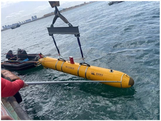
Figure 1.
Underwater experimental platform.
During underwater navigation, GPS is disabled. INS provides important attitude information and acceleration data, which are critical for the accurate underwater positioning of the AUV. DVL provides velocity data in the forward, right, and downward directions in the submersible’s coordinate system, which aids in effective navigation and positioning through data fusion filtering methods.
As illustrated in Figure 2, the navigation coordinate system employed in this study is the standard north–east–down (NED) system. Additionally, the AUV’s structural framework includes a secondary coordinate system described by XGY, representing the forward, rightward, and downward directions during AUV operations. This system is used for resolving local velocities and converting parameters between the geodetic and vehicle coordinate systems.
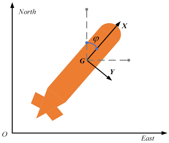
Figure 2.
AUV navigation coordinate system.
Following this, the paper constructs the system state vector and the observation vector within a framework for discrete-time state-space modeling. In this system, state vector is a nine-dimensional variable that describes the current state of the DR system. The state value at time can be described as
where , represents the position of the AUV in the NED coordinate system, and denotes the AUV’s heading in the geodetic coordinate system. , are the velocities of the AUV in the vehicle coordinate system. represents the angular velocity of the AUV, while are the accelerations in the and directions within the vehicle coordinate system. And is the angular acceleration. Since this system operates in discrete time, with being the navigation data sampling interval, the AUV state transition model is defined as follows:
where represents the process noise at time , denotes the state transition operator, and is the state value at time . The process noise is assumed to follow a zero-mean Gaussian distribution, , where is the process noise covariance matrix, expressed as
Furthermore, can be expressed in the following form:
The state value at time can be described as follows:
where is the AUV heading angle, are the forward and rightward velocities, is the measurement of angular velocity, and are the forward, rightward, and angular acceleration, respectively. The relationship between the measured values and state values is given by the following equation:
where represents the observation matrix, is a identity matrix, and denotes the measurement noise at time . Its covariance can be expressed as follows:
In practical underwater navigation, represents non-Gaussian noise, and is a time-varying measurement noise covariance matrix. Therefore, cannot be treated as a fixed value and must be processed using specific methods.
3. The Variational Bayesian Method and Mixed-Entropy-Based MEE-UKF Algorithm
Traditional underwater integrated navigation algorithms can be significantly impacted by sensor outliers and non-Gaussian noise, leading to large prediction errors and even filter divergence. Additionally, outliers in sensor observation data can severely affect the positioning accuracy of underwater vehicles. The original UKF based on the MMSE criterion may experience performance degradation when faced with these issues. In contrast, the MEE-UKF enhances the robustness of the AUV navigation algorithm under complex, non-Gaussian underwater disturbances by constructing and minimizing the error entropy function. However, due to inaccuracies in measuring the noise covariance matrix, the MEE-UKF can still result in significant prediction errors.
This paper presents a variational Bayesian method and mixed-entropy-based minimum error entropy unscented Kalman filter algorithm (VB-MMEE-UKF). This algorithm effectively addresses outliers and non-Gaussian noise while exhibiting robust performance and increased processing speed. These improvements significantly enhance the navigation accuracy of AUVs in complex and dynamic marine environments. The detailed aspects of the algorithm will be discussed in this section.
3.1. Minimum Error Entropy Criterion
The error between two random variables and is defined as . According to Renyi’s entropy [35], the error information can be expressed by the following equation:
In this equation, represents the order of Renyi’s entropy, and denotes the information potential, which can be expressed as
where denotes the probability density operator, which can be estimated in practical applications using the Parzen window [36] method:
where represents the number of error samples, which in this model can be considered as the total number of observations and state variables , denotes the error samples, and is the Gaussian kernel function, with being the user-defined kernel width. The Gaussian kernel function can be expressed as follows:
Based on the above equation, the estimation of the second-order information potential, denoted as , can be obtained.
Considering the negative logarithm function’s monotonically decreasing nature, reducing the error entropy in the second-order state implies maximizing the information potential . This means that by iteratively reducing the error entropy, one can effectively optimize the processing of noisy signals.
3.2. VB-MMEE-UKF Algorithmic Framework
3.2.1. Condition Prediction
To start, we need to construct a dynamic model based on Equations (2) and (6) mentioned above, assuming the dimensions of the state vector and measurement vector are represented by and , respectively. Both the MEE-UKF and the traditional UKF filters require the same process to perform the prior estimation of the state values. The estimation process is as follows:
Next, a UT is required to obtain the set of sigma points. Equation (14) illustrates the process of generating sigma points in the UKF algorithm. To acquire the prior state estimation from the sigma points, a weighted sampling process must be conducted, as shown in Equation (15):
where and represent the prior estimates of the state and covariance, respectively, denotes the covariance matrix, and and are the weights of the mean and covariance for the i-th sigma point, respectively. The weights can be calculated using the following equations:
Here, is a scaling parameter, defined as . The value of determines the distribution of the sampling points, while is a tuning parameter ensuring that the matrix remains positive semi-definite. The weight coefficient can be used to incorporate higher-order moments in the equations.
3.2.2. Measurement Updates
Substituting the obtained sigma points into the observation equation enables the calculation of the observation estimate , as well as the predicted system mean and the covariance .
Here, denotes the covariance matrix of the measurement errors.
However, in practical applications, the use of a constant measurement noise covariance can limit the filter’s efficiency in handling dynamic measurements. To mitigate the impact of inaccurate preset measurement noise matrices on navigation accuracy, this paper introduces an adaptive measurement error covariance matrix based on VB, which enhances the overall filtering performance of the algorithm and broadens its applicability. The joint posterior distribution of the AUV navigation system state and measurement noise covariance can be approximately represented using the VB principle:
In this context, represents the unknown approximated densities of the system state, and represents the measurement noise covariance. The VB method approximates these densities by reducing the Kullback–Leibler (KL) divergence between the observed distribution and the true distribution. The KL divergence can be described as follows:
To minimize the KL divergence, we define . The corresponding probability density distribution can be expressed as follows:
Here, and are non-zero scaling constants. The posterior probability distribution can be approximated as the product of a Gaussian distribution and an inverse Wishart (IW) distribution , as expressed in Equation (21):
The Gaussian distribution and the inverse Wishart (IW) distribution can be represented as follows:
In this equation, represents the degrees of freedom parameter, and represents the scale matrix of the IW distribution. Here, denotes the dimensionality of the state, and represents the matrix’s trace. Therefore, the mean of the IW distribution can be approximately considered as the measurement noise covariance
To synchronously generate the IW distribution during the time update step, the dynamic model can be defined as
Here, is the forgetting factor, where , and . and represent the prior values of the degrees of freedom parameter and the scale matrix, respectively. Their posterior values can be obtained using the following equations:
By employing the aforementioned approach, the VB method can be used to iteratively obtain the approximate in real time. Substituting this value into Equation (17) yields a more precise adaptive prediction mean .
3.2.3. Status Update
To apply the MEE criterion to the UKF, an augmented regression model must be formulated. Initially, the nonlinear measurement equation is linearized using a statistical linearization approach, yielding the following equation:
Here, denotes an identity matrix, and represents the augmented noise vector composed of state and measurement errors, which can be expressed as follows:
Based on Equation (28), we can perform a Cholesky decomposition to obtain the following result:
And can be decomposed as follows:
and can be obtained via Cholesky decomposition of the prior state covariance and the statistical linearization error with covariance [37]. Subsequently, by multiplying both sides of Equation (27) by , a normalized regression equation is derived, as shown below:
where and can be expressed by the following equation:
From this, assuming , we are informed
Substituting the above equation into Equation (13), we obtain the cost function as follows:
This study proposes a mixed error entropy with two Gaussian functions as the kernel to boost learning performance. Specifically, the minimum mixed error entropy can be defined as
Here, represents the mixing coefficient for the Gaussian kernel functions. It is noteworthy that the mixed error entropy can be generalized to cases involving more than two Gaussian functions. This study specifically focuses on the combination of two Gaussian kernel functions, under the assumption that .
Subsequently, the gradient of the cost function is calculated as follows:
The state can then be directly solved using the equation :
However, as indicated in [31], within the MEE-KF algorithm, the matrix being singular can cause numerical instability in the matrix . Therefore, the solution process for in Equation (40) can be estimated using the least squares (LS) method:
where . Substituting Equation (43) into Equation (42) yields
Subsequently, the state vector for the AUV can be further solved using the fixed-point iteration method:
where represents the result of the -th fixed-point iteration, and denotes the Kalman gain solved under the minimum error entropy criterion, which can be determined using the following equation:
Through fixed-point iteration, the stabilized is ultimately obtained, enabling the computation of the mean square error matrix:
Subsequently, the algorithm’s navigation-positioning functionality can be achieved through iteration. The VB-MMEE-UKF algorithm is summarized in Algorithm 1.
| Algorithm 1 VB-MMEE-UKF | |
| 1: | ; |
| 2: | by Equation (15); |
| 3: | by Equations (25) and (26); |
| 4: | = 1, 2, …, N |
| 5: | by Equation (24); |
| 6: | by Equation (17); |
| 7: | ; |
| 8: | by Equation (30); |
| 9: | by Equations (32) and (33); |
| 10: | = 1, 2, …, G |
| 11: | by Equation (34); |
| 12: | by Equations (38) and (39); |
| 13: | ; |
| 14: | by Equations (46)–(49) |
| 15: | by Equation (51); |
| 16: | by Equation (50) through fixed-point iteration; |
| 17: | |
| 18: | |
| 19: | end if |
| 20: | end for |
| 21: | by Equation (52); |
| 22: | end for |
| 23: | Repeat steps 2~22 until the navigation task is complete. |
4. Experimental Results and Simulation Analysis
The performance of the VB-MMEE-UKF was evaluated through simulations and compared with several established algorithms: the unscented Kalman filter (UKF), the iterative maximum mixed correlation unscented Kalman filter (IMMCUKF), the minimum error entropy unscented Kalman filter (MEE-UKF), and the variational Bayes minimum error entropy unscented Kalman filter (VB-MEE-UKF). Each of these algorithms was applied to the AUV navigation model which was introduced in Section 2.
4.1. Simulation Setup and Data Analysis
In order to assess the performance of the algorithm in a simulated environment, we utilized the previously proposed AUV dynamic model to generate synthetic data. Multiple simulation experiments were conducted to comprehensively assess each algorithm’s performance. The performance of each algorithm is quantified by the root mean square error (RMSE) of the endpoints and average root mean square error (ARMSE), which are calculated as follows:
where represents the AUV position calculated using different algorithms in the geodetic coordinate system, while represents the true AUV position in the geodetic coordinate system. denotes the total length of the dataset, and indicates the number of Monte Carlo runs. The following sections will present the parameter settings used in the simulation experiments for the algorithms.
The initial covariance matrix for process noise , the initial covariance matrix for measurement noise , and the initial state covariance matrix are provided by Equation (56):
The parameters of UKF in Equation (16) are as follows:
The bandwidth of a single Gaussian kernel is set to . The bandwidths of the two kernels and their mixing weights for the mixed Gaussian kernel are set as follows:
The initial parameters of the VB method are set as follows:
The termination criterion for the fixed-point iteration is set to .
In all simulation scenarios, the AUV operates for 1000 steps, with each step corresponding to one second of motion in a 2D flat area. The AUV starts from the initial position , with an initial heading of 0°, maintaining a constant forward velocity of 1 m/s.
The effectiveness of the algorithm was validated using simulation cases with two different trajectories based on the aforementioned equations. Simulation Case 1, illustrated in Figure 3a, generated a hexagonal trajectory using the AUV dynamic model. Angle accelerations of were applied at intervals of 150–160 s, 310–320 s, 470–480 s, 630–640 s, 790–800 s, and 950–960 s, and angle accelerations of −0.6°/s2 were applied at intervals of 160–170 s, 320–330 s, 480–490 s, 640–650 s, 800–810 s, and 960–970 s to achieve multiple turns during the AUV’s operation. The complete trajectory formation took 1000 s, covering 1000 m at a default forward speed of 1 m/s.
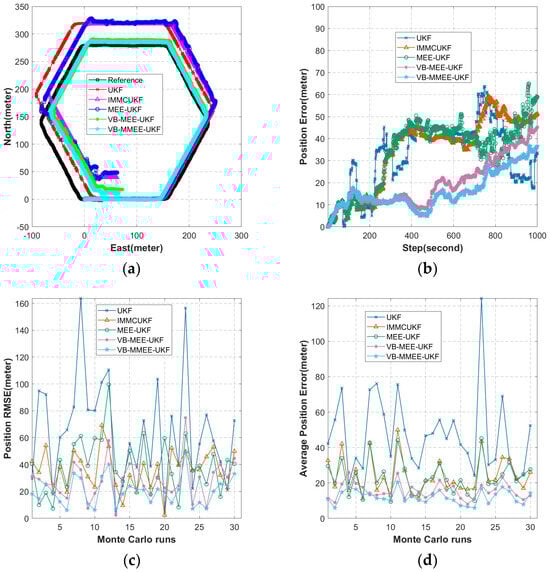
Figure 3.
Experimental data for Simulation Case 1: (a) experimental trajectory diagram; (b) algorithmic pushover error map; (c) endpoint RMSE of 30 Monte Carlo simulations; (d) ARMSE of 30 Monte Carlo simulations.
Simulation Case 2, illustrated in Figure 4a, generated a quadrilateral trajectory using the aforementioned AUV dynamic model. Angular accelerations of were applied at intervals of 240–250 s, 490–500 s, and 740–750 s, while angular accelerations of −0.9°/s2 were applied at intervals of 250–260 s, 500–510 s, and 750–760 s to achieve multiple turns during the AUV’s operation. The complete trajectory formation took 1000 s, covering 1000 m at a default forward speed of 1 m/s.
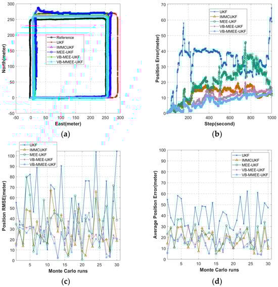
Figure 4.
Experimental data for Simulation Case 2: (a) experimental trajectory diagram; (b) algorithmic pushover error map; (c) endpoint RMSE of 30 Monte Carlo simulations; (d) ARMSE of 30 Monte Carlo simulations.
Unlike Cases 1 and 2, Case 3, illustrated in Figure 5a, assigned a constant angular velocity of 0.36°/s throughout the AUV’s motion. This resulted in a circular trajectory over the entire duration. The complete trajectory formation took 1000 s, covering 1000 m at a default forward speed of 1 m/s.
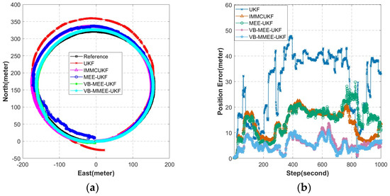
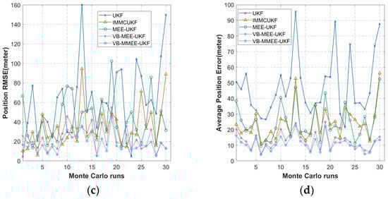
Figure 5.
Experimental data for Simulation Case 3: (a) experimental trajectory diagram; (b) algorithmic pushover error map; (c) endpoint RMSE of 30 Monte Carlo simulations; (d) ARMSE of 30 Monte Carlo simulations.
Additionally, during the simulation process, the DVL measurements were subjected to a multi-Gaussian noise model to simulate the relatively harsh measurement noise environment found in marine conditions. Consequently, the trajectory estimations of all algorithms were subject to some degree of interference.
The simulation program was executed using MATLAB R2022b on a computer with an R9-7945HX processor, RTX 4060 GPU, and 16.0 GB of RAM.
The resulting statistical data are summarized in Table 1.

Table 1.
Simulation result statistics of the algorithm.
Table 1 highlights the improvements achieved by our proposed algorithm across 30 Monte Carlo simulations. In Case 1, the endpoint-position accuracy RMSE improved by 55.49% relative to the UKF, 21.33% relative to the IMMCUKF, 44.41% relative to the MEE-UKF, and 12.93% relative to the VB-MEE-UKF. Moreover, overall navigation accuracy saw enhancements of 68.41% relative to the UKF, 37.52% relative to the IMMCUKF, 44.31% relative to the MEE-UKF, and 3.46% relative to the VB-MEE-UKF.
In Case 2, our algorithm improved endpoint-position RMSE by 55.77% relative to the UKF, 18.85% relative to the IMMCUKF, 33.41% relative to the MEE-UKF, and 10.91% relative to the VB-MEE-UKF. Navigation accuracy also saw improvements of 61.41% relative to the UKF, 17.19% relative to the IMMCUKF, 27.40% relative to the MEE-UKF, and 6.46% relative to the VB-MEE-UKF.
For Case 3, the endpoint-position RMSE was improved by 70.47% relative to the UKF, 47.12% relative to the IMMCUKF, 56.93% relative to the MEE-UKF, and 23.58% relative to the VB-MEE-UKF. Overall navigation accuracy improved by 76.82% relative to the UKF, 54.13% relative to the IMMCUKF, 55.36% relative to the MEE-UKF, and 14.72% relative to the VB-MEE-UKF.
Drawing upon the statistical outcomes derived from the simulation experiments, we can conclude that our proposed algorithm is suitable for practical engineering applications and demonstrates significant effectiveness in suppressing non-Gaussian noise, exhibiting superior robustness compared to other existing algorithms. Additionally, Table 1 records the maximum computation time per step for each algorithm during the operation. While our proposed algorithm necessitates extended processing time, it still meets the frequency requirements for practical engineering applications.
4.2. Analysis of Data Obtained from Maritime Field Trials
We utilized sea trial data collected from the PX-260 underwater vehicle to compare the performance of the proposed algorithm with other existing algorithms.
The PX-260 AUV developed by the Qingdao Underwater Vehicle Laboratory in Shandong, China, is equipped with a range of navigation sensors, including GPS, INS, depth sensors, and DVLs, which collect real-time navigational information during underwater missions. The PX-260’s built-in industrial control computer communicates in real time with the various navigation sensors via serial or network ports and uses algorithms to determine the AUV’s current position for autonomous positioning and navigation. The PX-260 operating status is shown in Figure 6. The metrics of the navigation sensors used in this are shown in Table 2.
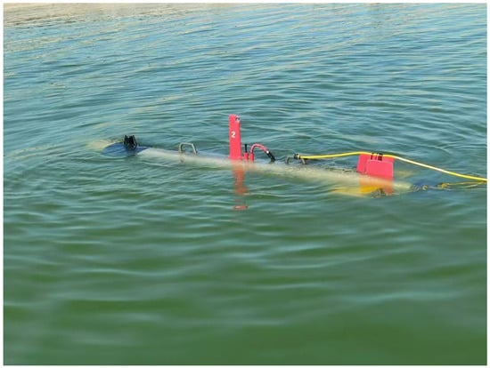
Figure 6.
PX-260 AUV work process.
Table 2.
PX-260 AUV sensor performance.
By artificially introducing a commonly used multi-Gaussian model framework into the sensor data, we simulate the relatively harsh measurement noise environment found in marine conditions. Repeating the experiments under these conditions allows for a clearer demonstration of the algorithm’s effectiveness.
During the sea trials, the AUV traveled over the water at approximately 2 knots, thus acquiring GPS data as a standard value for the outputs and obtaining the measurements required by the algorithm through sensors such as the INS and the DVL to perform the waypoint derivation. The performance results of the algorithm are presented below:
The statistical results of the sea trial data are shown in Table 3. As shown in Figure 7, sea trial data 1, our proposed algorithm improves the root mean square error of the endpoint position by 44.31% compared to UKF, 19.51% compared to IMMCUKF, 33.07% compared to MEE-UKF, and 9.92% compared to VB-MEE-UKF. In addition, the overall navigation accuracy is improved by 46.53% compared to UKF, 25.23% compared to IMMCUKF, 34.86% compared to MEE-UKF, and 12.19% compared to VB-MEE-UKF. From these statistical results, we conclude that the proposed algorithm is very suitable for practical engineering applications, can effectively suppress non-Gaussian noise, and has stronger robustness compared with existing algorithms.
Table 3.
Validation of different algorithms on sea trial data.
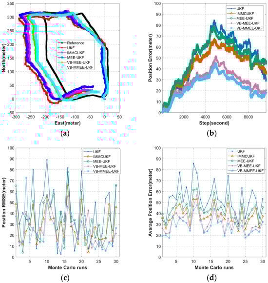
Figure 7.
Experimental data from Sea Trial Data 1: (a) experimental trajectory diagram; (b) algorithmic pushover error map; (c) endpoint RMSE of 30 Monte Carlo simulations; (d) ARMSE of 30 Monte Carlo simulations.
In sea trial data 2 in Figure 8, unknown disturbances clearly impacted the performance of various algorithms. However, our proposed algorithm effectively mitigated this degradation. The endpoint-position RMSE of our algorithm showed a 50.17% improvement compared to the UKF, 21.07% compared to the IMMCUKF, 37.01% compared to the MEE-UKF, and 12.77% compared to the VB-MEE-UKF. Furthermore, the overall navigation accuracy improved by 41.10% compared to the UKF, 13.19% compared to the IMMCUKF, 27.05% compared to the MEE-UKF, and 12.71% compared to the VB-MEE-UKF. Based on these statistical results, we conclude that our algorithm outperforms existing methods for underwater vehicle navigation in the presence of disturbances.
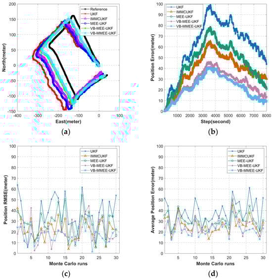
Figure 8.
Experimental data from Sea Trial Data 2: (a) experimental trajectory diagram; (b) algorithmic pushover error map; (c) endpoint RMSE of 30 Monte Carlo simulations; (d) ARMSE of 30 Monte Carlo simulations.
5. Conclusions
In this paper, a VB-MMEE-UKF algorithm for underwater vehicle navigation and localization is proposed. By integrating the VB method of adaptive optimization of measurement covariance and the hybrid minimum error entropy technique, the accuracy of the AUV navigation system is enhanced and the robustness to outliers is improved. The performance of the method is verified by simulation and sea trial data and compared to the conventional UKF, IMMCUKF, MEE-UKF, and VB-MEE-UKF algorithms. The experimental results show that compared to the existing algorithms, the overall navigation accuracy of this paper’s algorithm is improved by at least 10%, which proves the effectiveness and robustness of the proposed method. Although the algorithm can meet the real-time navigation requirements at certain frequencies, it has a longer computation time compared with the traditional methods. Future research will focus on increasing the computational speed of the algorithm to further improve its performance. In addition, the kernel function form of the minimum error entropy will be further explored to enable various MEE-based methods to deal with more complex environments, thus improving underwater navigation and localization performance.
Author Contributions
Conceptualization, B.J. and X.S.; methodology, B.J.; software, B.J.; validation, B.J., P.C. and S.W.; formal analysis, B.J.; investigation, B.J.; resources, B.H.; data curation, B.J. and S.S.; writing—original draft preparation, B.J.; writing—review and editing, B.J.; supervision, B.H.; project administration, B.H. All authors have read and agreed to the published version of the manuscript.
Funding
This research received no external funding.
Data Availability Statement
The data presented in this study are available upon request from the corresponding author. The data are not publicly available because they are part of ongoing research and development.
Acknowledgments
The authors would like to thank Bo He, Xiaona Sun, and Peimiao Chen for their technical support and the editors and reviewers for their useful comments.
Conflicts of Interest
The authors declare no conflicts of interest.
References
- Song, S.; Liu, J.; Guo, J.; Wang, J.; Xie, Y.; Cui, J.H. Neural-network-based AUV navigation for fast-changing environments. IEEE Internet Things J. 2020, 7, 9773–9783. [Google Scholar] [CrossRef]
- Paull, L.; Saeedi, S.; Seto, M.; Li, H. Sensor-driven online coverage planning for autonomous underwater vehicles. IEEE/ASME Trans. Mechatron. 2012, 18, 1827–1838. [Google Scholar] [CrossRef]
- Leonard, J.J.; Bahr, A. Autonomous underwater vehicle navigation. In Springer Handbook of Ocean Engineering; Springer: Berlin/Heidelberg, Germany, 2016; pp. 341–358. [Google Scholar]
- Han, J.; Ma, C.; Zou, D.; Jiao, S.; Chen, C.; Wang, J. Distributed Multi-Robot SLAM Algorithm with Lightweight Communication and Optimization. Electronics 2024, 13, 4129. [Google Scholar] [CrossRef]
- Zhang, X.; He, B.; Gao, S.; Mu, P.; Xu, J.; Zhai, N. Multiple model AUV navigation methodology with adaptivity and robustness. Ocean Eng. 2022, 254, 111258. [Google Scholar] [CrossRef]
- Paull, L.; Saeedi, S.; Seto, M.; Li, H. AUV navigation and localization: A review. IEEE J. Ocean. Eng. 2013, 39, 131–149. [Google Scholar] [CrossRef]
- Huang, Y.; Zhang, Y.; Xu, B.; Wu, Z.; Chambers, J.A. A new adaptive extended Kalman filter for cooperative localization. IEEE Trans. Aerosp. Electron. Syst. 2017, 54, 353–368. [Google Scholar] [CrossRef]
- Sabet, M.T.; Daniali, H.M.; Fathi, A.; Alizadeh, E. A low-cost dead reckoning navigation system for an AUV using a robust AHRS: Design and experimental analysis. IEEE J. Ocean. Eng. 2017, 43, 927–939. [Google Scholar] [CrossRef]
- Huang, Y.; Zhang, Y. A new process uncertainty robust Student’s t-based Kalman filter for SINS/GPS integration. IEEE Access 2017, 5, 14391–14404. [Google Scholar] [CrossRef]
- Li, X.; Zhang, J. Innovation Adaptive UKF Train Location Method Based on Kinematic Constraints. Electronics 2024, 13, 3958. [Google Scholar] [CrossRef]
- Uhlmann, J.K. Algorithms for multiple-target tracking. Am. Sci. 1992, 80, 128–141. [Google Scholar]
- Lu, J.; Zhang, T.; Hu, F.; Hao, Q. Preprocessing design in pyroelectric infrared sensor-based human-tracking system: On sensor selection and calibration. IEEE Trans. Syst. Man Cybern. Syst. 2016, 47, 263–275. [Google Scholar] [CrossRef]
- Chen, S.Y. Kalman filter for robot vision: A survey. IEEE Trans. Ind. Electron. 2011, 59, 4409–4420. [Google Scholar] [CrossRef]
- Yang, X.; Zhang, W.A.; Yu, L. A bank of decentralized extended information filters for target tracking in event-triggered WSNs. IEEE Trans. Syst. Man Cybern. Syst. 2019, 50, 3281–3289. [Google Scholar] [CrossRef]
- Bucci, A.; Franchi, M.; Ridolfi, A.; Secciani, N.; Allotta, B. Evaluation of UKF-based fusion strategies for autonomous underwater vehicles multisensor navigation. IEEE J. Ocean. Eng. 2022, 48, 1–26. [Google Scholar] [CrossRef]
- Cantelobre, T.; Chahbazian, C.; Croux, A.; Bonnabel, S. A real-time unscented Kalman filter on manifolds for challenging AUV navigation. In Proceedings of the 2020 IEEE/RSJ International Conference on Intelligent Robots and Systems (IROS), Las Vegas, NV, USA, 25 October 2020; pp. 2309–2316. [Google Scholar]
- Choi, M.; Seo, M.; Kim, H.S.; Seo, T. UKF-based sensor fusion method for position estimation of a 2-DOF rope driven robot. IEEE Access 2021, 9, 12301–12308. [Google Scholar] [CrossRef]
- Filipovic, V.; Nedic, N.; Stojanovic, V. Robuste Identifikation von pneumatischen Servo-Aktuatoren in der realen Situationen. Forsch. Ingenieurwes. 2011, 75, 183–196. [Google Scholar] [CrossRef]
- Xie, Y.; Li, Y.; Gu, Y.; Cao, J.; Chen, B. Fixed-point minimum error entropy with fiducial points. IEEE Trans. Signal Process. 2020, 68, 3824–3833. [Google Scholar] [CrossRef]
- Chen, B.; Dang, L.; Gu, Y.; Zheng, N.; Príncipe, J.C. Minimum error entropy Kalman filter. IEEE Trans. Syst. Man Cybern. 2019, 51, 5819–5829. [Google Scholar] [CrossRef]
- Wang, G.; Xue, R.; Wang, J. A distributed maximum correntropy Kalman filter. Signal Process. 2019, 160, 247–251. [Google Scholar] [CrossRef]
- Liu, X.; Ren, Z.; Lyu, H.; Jiang, Z.; Ren, P.; Chen, B. Linear and nonlinear regression-based maximum correntropy extended Kalman filtering. IEEE Trans. Syst. Man Cybern. Syst. 2019, 51, 3093–3102. [Google Scholar] [CrossRef]
- Li, P.; Sun, X.; Chen, Z.; Zhang, X.; Yan, T.; He, B. A Robust and Adaptive AUV Integrated Navigation Algorithm Based on a Maximum Correntropy Criterion. Electronics 2024, 13, 2426. [Google Scholar] [CrossRef]
- Liu, W.; Pokharel, P.P.; Principe, J.C. Correntropy: Properties and applications in non-Gaussian signal processing. IEEE Trans. Signal Process. 2007, 55, 5286–5298. [Google Scholar] [CrossRef]
- Chen, B.; Príncipe, J.C. Maximum correntropy estimation is a smoothed MAP estimation. IEEE Signal Process. Lett. 2012, 19, 491–494. [Google Scholar] [CrossRef]
- Erdogmus, D.; Principe, J.C. An error-entropy minimization algorithm for supervised training of nonlinear adaptive systems. IEEE Trans. Signal Process. 2002, 50, 1780–1786. [Google Scholar] [CrossRef]
- Zhang, Y.; Chen, B.; Liu, X.; Yuan, Z.; Principe, J.C. Convergence of a fixed-point minimum error entropy algorithm. Entropy 2015, 17, 5549–5560. [Google Scholar] [CrossRef]
- Erdogmus, D.; Principe, J.C. Generalized information potential criterion for adaptive system training. IEEE Trans. Neural Netw. 2002, 13, 1035–1044. [Google Scholar] [CrossRef] [PubMed]
- Silva, L.M.; Felgueiras, C.S.; Alexandre, L.A.; de Sá, J.M. Error entropy in classification problems: A univariate data analysis. Neural Comput. 2006, 18, 2036–2061. [Google Scholar] [CrossRef]
- Santamaría, I.; Erdogmus, D.; Principe, J.C. Entropy minimization for supervised digital communications channel equalization. IEEE Trans. Signal Process. 2002, 50, 1184–1192. [Google Scholar] [CrossRef]
- Wang, G.; Chen, B.; Yang, X.; Peng, B.; Feng, Z. Numerically stable minimum error entropy Kalman filter. Signal Process. 2021, 181, 107914. [Google Scholar] [CrossRef]
- Dang, L.; Chen, B.; Wang, S.; Ma, W.; Ren, P. Robust power system state estimation with minimum error entropy unscented Kalman filter. IEEE Trans. Instrum. Meas. 2020, 69, 8797–8808. [Google Scholar] [CrossRef]
- Li, M.; Jing, Z.; Leung, H. Robust minimum error entropy based cubature information filter with non-Gaussian measurement noise. IEEE Signal Process. Lett. 2021, 28, 349–353. [Google Scholar] [CrossRef]
- He, J.; Wang, G.; Peng, B.; Sun, Q.; Feng, Z.; Zhang, K. Mixture quantized error entropy for recursive least squares adaptive filtering. J. Frankl. Inst. 2022, 359, 1362–1381. [Google Scholar] [CrossRef]
- Sahoo, P.; Wilkins, C.; Yeager, J. Threshold selection using Renyi’s entropy. Pattern Recognit. 1997, 30, 71–84. [Google Scholar] [CrossRef]
- Kwak, N.; Choi, C.-H. Input feature selection by mutual information based on Parzen window. IEEE Trans. Pattern Anal. Mach. Intell. 2002, 24, 1667–1671. [Google Scholar] [CrossRef]
- Zhao, J.; Mili, L. A robust generalized-maximum likelihood unscented Kalman filter for power system dynamic state estimation. IEEE J. Sel. Top. Signal Process. 2018, 12, 578–592. [Google Scholar] [CrossRef]
Disclaimer/Publisher’s Note: The statements, opinions and data contained in all publications are solely those of the individual author(s) and contributor(s) and not of MDPI and/or the editor(s). MDPI and/or the editor(s) disclaim responsibility for any injury to people or property resulting from any ideas, methods, instructions or products referred to in the content. |
© 2024 by the authors. Licensee MDPI, Basel, Switzerland. This article is an open access article distributed under the terms and conditions of the Creative Commons Attribution (CC BY) license (https://creativecommons.org/licenses/by/4.0/).