Combination of a Rabbit Optimization Algorithm and a Deep-Learning-Based Convolutional Neural Network–Long Short-Term Memory–Attention Model for Arc Sag Prediction of Transmission Lines

Abstract

Arc droop presents significant challenges in power system management due to its inherent complexity and dynamic nature. To address these challenges in predicting arc sag for transmission lines, this paper proposes an innovative time–series prediction model, AROA-CNN-LSTM-Attention(AROA-CLA). The model aims to enhance arc sag prediction by integrating a convolutional neural network (CNN), a long short-term memory network (LSTM), and an attention mechanism, while also utilizing, for the first time, the adaptive rabbit optimization algorithm (AROA) for CLA parameter tuning. This combination improves both the prediction performance and the generalization capability of the model. By effectively leveraging historical data and exhibiting superior time–series processing capabilities, the AROA-CLA model demonstrates excellent prediction accuracy and stability across different time scales. Experimental results show that, compared to traditional and other modern optimization models, AROA-CLA achieves significant improvements in RMSE, MAE, MedAE, and R² metrics, particularly in reducing errors, accelerating convergence, and enhancing robustness. These findings confirm the effectiveness and applicability of the AROA-CLA model in arc droop prediction, offering novel approaches for transmission line monitoring and intelligent power system management.

1. Introduction

Amid the continuous growth of global power demand and the increasing complexity of grid loads, ensuring stable operation and precise monitoring of transmission lines has become a pivotal task in power system management [1]. Arc sag, a crucial parameter for transmission lines, significantly influences the safety and operational efficiency of power grids and is integral to system fault prediction and prevention [2]. However, arc sag is impacted by various factors such as ambient temperature, load fluctuations, wind speed, humidity, and line aging, all of which contribute to its significant nonlinear and non-smooth characteristics. These complexities pose challenges for traditional linear prediction models, making them less effective in addressing such dynamic changes. Consequently, developing intelligent algorithms that can precisely capture the intricate timing characteristics and deliver high-precision predictions has become a crucial research direction for enhancing the intelligence of power systems.

In recent years, the development and innovative application of technology have led to the proposal of various advanced methods for arc sag monitoring of transmission lines. For instance, Wang D et al. [3] proposed a method for monitoring arc sag in iced transmission lines using stereo vision technology, which enables accurate 3D reconstruction and monitoring of overhead transmission lines. This technique is crucial for maintaining grid security under freezing conditions. Similarly, Song J et al. [4] introduced a method for arc sag measurement based on unmanned aerial vehicle (UAV) aerial photography and deep learning techniques. The study proposed an automatic isolation bar segmentation algorithm, CM–Mask–RCNN, which integrates a CAB attention mechanism and MHSA self-attention mechanism to automatically extract isolation bars and compute their center coordinates. By combining conventional algorithms, such as beam method leveling, spatial pre-convergence, and spatial curve fitting, this method provides cost-effective arc droop measurements. Wydra M et al. [5] proposed a vision-based system utilizing LoRa communication for monitoring slack and temperature in overhead transmission lines. This method captures images from cameras mounted on poles and processes them to obtain slack and temperature data, thus preventing disconnections during installation or maintenance. Long X et al. [6] applied Bayesian optimization (BO) and XGBoost models to predict the jump height of transmission lines after de-icing. By performing numerical studies under various structural, icing, and wind conditions, the BO-XGBoost model outperforms other machine learning models, offering a reliable, efficient, and interpretable tool for designing safer transmission line systems in freezing conditions. Finally, Wang J et al. [7] proposed Boosted DETR, an end-to-end sensing framework for UAV inspection of transmission lines. This framework uses a detection transformer (DETR) model and an enhanced multi-scale Retinex algorithm to optimize object detection, improving the recognition accuracy of small critical components, such as insulators and anti-vibration hammers, in complex environments. The framework aims to enhance the efficiency and accuracy of transmission line inspections while adapting to changing environmental conditions.

Deep learning techniques, particularly long short-term memory networks (LSTMs) [8], have demonstrated robust modeling capabilities for time–series prediction tasks. For instance, Jun Liu et al. [9] introduced an innovative LSTM model known as Global Context-Aware Attention LSTM (GCA-LSTM) for human action recognition based on skeletal sequences. Additionally, Fazle Karim et al. [10] developed a hybrid model that combines fully convolutional neural networks (FCNs) and long short-term memory networks (LSTMs) for time–series classification tasks, known as LSTM-FCN and ALSTM-FCN. Furthermore, Weicong Kong et al. [11] proposed an LSTM-based recurrent neural network for short-term residential load forecasting, addressing the prediction challenges for individual residential users.

LSTM has been extensively employed in various domains such as finance, weather forecasting, and speech recognition, due to its unique structure that captures both long-term and short-term data dependencies. For instance, Haojun Pan et al. [12] developed an innovative hybrid model that integrates a long short-term memory (LSTM) network with a generalized autoregressive conditional heteroskedasticity (GARCH) model to predict stock index futures prices. Similarly, Jun Luo et al. [13] combined an ARIMA model, the Whale Optimization Algorithm (WOA), and LSTM to enhance air pollution management by accurately forecasting air pollutant concentrations. Additionally, Ruben Zazo et al. [14] utilized LSTM-based recurrent neural networks (RNNs) for automatic language identification, which is particularly effective in scenarios involving very short utterances, such as those under three seconds. These applications highlight the adaptability of LSTM in handling various challenges, including those in power systems. Nevertheless, the single LSTM model often struggles with capturing complex feature interactions and nonlinear variations in multidimensional data. In contexts such as arc droop prediction in transmission lines, where multiple factors influence the outcomes, a more sophisticated modeling approach is essential to address the shortcomings of conventional models in processing high-dimensional dynamic features.

Parameters in power systems often exhibit significant aggregation effects and irregular fluctuations, where subtle variations can profoundly influence prediction outcomes and system operational decisions. In response to these challenges, several advanced composite models incorporating convolutional neural networks (CNNs) and attention mechanisms have been developed. For instance, Kun Xia et al. [15] introduced a deep learning model that combines long short-term memory (LSTM) and CNNs for human activity recognition (HAR). Similarly, Toon Bogaerts et al. [16] designed a graph CNN-LSTM neural network for predicting both short and long-term traffic flows based on trajectory data from urban road networks. Furthermore, Ranjan Kumar Behera et al. [17] developed a novel hybrid model that merges CNNs and LSTM networks for sentiment analysis tasks in social media. These methods have demonstrated considerable potential in extracting local features and global dependencies. However, optimizing these models to better suit the complex, multidimensional time–series data needs in power systems remains a pressing research challenge [18].

This paper introduces an innovative composite prediction model that integrates a convolutional neural network (CNN), an attention mechanism, and the adaptive rabbit optimization algorithm (AROA). This model targets high-precision predictions of critical parameters such as arc sag in transmission lines. Initially, the CNN extracts local features from input data and identifies short-term fluctuation patterns within the time–series. Subsequently, long-term dependencies are captured by an CNN–LSTM–Attention network to develop a comprehensive feature representation. To enhance model performance further, the AROA, which simulates the foraging and avoidance behaviors of rabbits, is employed to intelligently search and optimize hyperparameters. This algorithm dynamically balances global exploration and local exploitation in the search space, effectively preventing convergence to locally optimal solutions and thus boosting the model’s prediction accuracy and generalization capability. Meanwhile, the attention mechanism focuses the model’s awareness on crucial moments within the time–series, facilitating a deeper understanding and processing of complex temporal data. Additionally, this paper outlines the following key contributions.

(1)

Optimization of the ROA algorithm: Building on improvements to the traditional ROA algorithm, the AROA algorithm incorporates dynamic energy coefficients and a differential variance strategy. These enhancements effectively improve the algorithm’s global exploration and local exploitation capabilities, significantly increasing the model’s convergence speed and optimization efficiency.

(2)

Proposing a novel prediction model: This paper presents the integration of the adaptive rabbit optimization algorithm (AROA) into the CNN–LSTM–Attention model for the first time, creating the AROA–CNN–LSTM–Attention (AROA-CLA) model. The AROA algorithm enhances prediction accuracy and stability by optimizing model parameters.

(3)

Innovative introduction of a multi-correlated target variable forecasting model: This model combines data from multivariate time–series, allowing it to more effectively capture the joint variations of the target variable and its correlated factors, thereby enhancing the adaptability of arc droop forecasting in complex environments.

2. Materials and Methods

2.1. Adaptive Rabbit Optimization Algorithm

The rabbits optimization algorithm (ROA) is a novel meta-heuristic algorithm inspired by the foraging and hiding behaviors of rabbits. The algorithm simulates rabbits’ survival strategies in nature, such as detour foraging and random hiding, to locate the global optimal solution within a complex search space. ROA employs the foraging behavior of rabbits for global exploration and their hiding behavior for local exploitation, achieving a smooth transition between the two through the gradual decay of an energy factor. This design makes ROA well-balanced and adaptable, enabling it to achieve superior solutions across various optimization problems. Building on this background, ROA solves optimization problems through six core steps: population initialization, energy factor control, detour foraging, random hiding, position updating, and termination.

2.1.1. Population Initialization

In ROA, a set of individual rabbits is initially generated, where the position of each rabbit represents a candidate solution. These locations are randomly assigned within the search space to ensure a diverse initial population, thereby enhancing the potential for global exploration. First, nnn individual rabbits are generated, each with a position randomly distributed within the search space bounds [lower_bound,upper_bound]. The global best solution and fitness values are then initialized to support subsequent solution updates and comparisons [19].

2.1.2. Calculation of Energy Factor A

Energy factor A controls the search behavior of the algorithm at each iteration, simulating the rabbit’s energy consumption during foraging and hiding. As the number of iterations increases, the energy factor gradually decreases, guiding the algorithm’s transition from global exploration to local exploitation. The energy factor is calculated as follows:

$$\mathrm{A}\left(\mathrm{t}\right)=4\left(1-{\displaystyle \frac{\mathrm{t}}{\mathrm{T}}}\right)\ln \left({\displaystyle \frac{1}{\mathrm{r}}}\right)$$

(1)

$t$ is the current number of iterations. $T$ is the maximum number of iterations. $r$ is a random number used to introduce uncertainty. When A > 1, the algorithm enters global exploration (foraging in a roundabout way); when A ≤ 1, the algorithm enters local exploitation (random hiding).

2.1.3. Detour Foraging–Global Exploration

When energy factor A > 1, the algorithm simulates the detour foraging behavior of rabbits, where they forage in areas distant from their nest to avoid local minima traps. This strategy enhances the algorithm’s global search capability.

$${\mathrm{v}}_{\mathrm{i}}\left(\mathrm{t}+1\right)={\mathrm{x}}_{\mathrm{j}}\left(\mathrm{t}\right)+\mathrm{R}·\left({\mathrm{x}}_{\mathrm{i}}\left(\mathrm{t}\right)-{\mathrm{x}}_{\mathrm{j}}\left(\mathrm{t}\right)\right)+\mathrm{round}\left(0.5·\left(0.05+{\mathrm{r}}_1\right)\right)·{\mathrm{n}}_1$$

(2)

${\mathrm{x}}_{\mathrm{i}}\left(\mathrm{t}\right)$ and ${\mathrm{x}}_{\mathrm{j}}\left(\mathrm{t}\right)$ are run operators that control the direction of the rabbit’s movement and the step size. $R$ is a run operator that controls the direction of the rabbit’s movement and the step size. $r_1$ is a random number that is used to increase the randomness of the exploration. ${\mathrm{n}}_1\sim \mathrm{N}\left(0,1\right)$ is a perturbation term of the standard normal distribution that prevents from falling into the local extremes. The detour foraging strategy allows the rabbit to explore over a large area and helps to discover potential global optimal solutions in the search space.

2.1.4. Random Hiding–Local Development

When energy factor A ≤ 1, the algorithm simulates the rabbit’s random hiding behavior. In this phase, the rabbit randomly selects one of multiple hiding locations, enabling a more refined search within the local area:

$${\mathrm{b}}_{\mathrm{i},\mathrm{j}}\left(\mathrm{t}\right)={\mathrm{x}}_{\mathrm{i}}\left(\mathrm{t}\right)+\mathrm{H}·\mathrm{g}·{\mathrm{x}}_{\mathrm{i}}\left(\mathrm{t}\right)$$

(3)

In this algorithm, ${\mathrm{b}}_{\mathrm{i},\mathrm{j}}\left(\mathrm{t}\right)$ represents the hiding position of rabbit i in dimension j. The hiding parameter, $\mathrm{H}={\displaystyle \frac{\mathrm{T}-\mathrm{t}+1}{\mathrm{T}}}·{\mathrm{r}}_4$ decreases with each iteration, ensuring that the algorithm focuses on local search in the later stages. The mapping vector g specifies the dimensions in which the hiding position is updated.

2.1.5. Location Updates

Each rabbit is assigned a candidate position after performing either detour foraging or random hiding. If the fitness of the candidate position is better than that of the current solution, the rabbit’s position is updated to the candidate position; otherwise, it remains in its original location.

$${\mathrm{x}}_{\mathrm{i}}\left(\mathrm{t}+1\right)=\left\{\begin{array}{ll}{\mathrm{v}}_{\mathrm{i}}\left(\mathrm{t}+1\right)\hfill & \mathrm{iff}\left({\mathrm{v}}_{\mathrm{i}}\left(\mathrm{t}+1\right)\right)<\mathrm{f}\left({\mathrm{x}}_{\mathrm{i}}\left(\mathrm{t}\right)\right)\hfill \\ {\mathrm{x}}_{\mathrm{i}}\left(\mathrm{t}\right)\hfill & \mathrm{otherwise}\hfill \end{array}\right.$$

(4)

Here, $f$ represents the fitness function, used to evaluate the quality of each solution.

2.1.6. Termination Conditions

At the end of each iteration, the algorithm checks whether the maximum number of iterations T has been reached. If the maximum number has been reached, the algorithm stops and outputs the current global best solution; otherwise, it proceeds to the next iteration.

2.1.7. Calculation of Adaptive Energy Factor A

The rabbit optimization algorithm has been improved to become the adaptive rabbit optimization algorithm. The specific parts of the improvement are detailed in the following.

In the original algorithm, energy factor A gradually decays to balance exploration and exploitation. To enhance adaptability, the energy factor can be dynamically adjusted based on population diversity: when diversity decreases, the algorithm increases exploration to avoid premature convergence. The formula for the dynamic energy factor is as follows:

$$\mathrm{A}\left(\mathrm{t}\right)=4\left(1-{\displaystyle \frac{\mathrm{t}}{\mathrm{T}}}\right)\ln \left({\displaystyle \frac{1}{\mathrm{r}}}\right)·\left(1+\mathrm{diversity}\right)$$

(5)

Here, $t$ represents the current iteration number, and $T$ is the maximum number of iterations. The variable $r$ is a random number introduced to add randomness, while “diversity” denotes population diversity, measuring the degree of variation within the current population. Lower diversity results in a higher energy factor, enhancing global exploration.

2.1.8. Adaptive Detour for Food—Global Exploration

Improvement: In the detour foraging phase, the step length R can be dynamically adjusted according to the iteration process and population diversity. Initially, a larger step length is used to cover a wider search space, while in the later stages, the step length is gradually reduced to allow for fine-grained local exploitation. Dynamic step size adjustment is applied to the step size factor R(t), based on population diversity, with the global best position added as an additional reference to guide individuals closer to the current optimal solution.

$$R\left(t\right)=\left(e-e^{{\left(\frac{t-1}{T}\right)}^2}\right)·\sin \left(2\pi r_2\right)·\left(1+\mathrm{diversity}\right)$$

(6)

The constant $e$ controls the dynamics of the step size, while $r_2$ is a random number that adds variability to the step size. “Diversity” denotes population diversity, initially setting a larger step size to enhance global exploration and gradually decreasing it in later stages to improve the precision of local exploitation.

Each rabbit references not only the position of a randomly selected rabbit but also the current global best position, ${\mathrm{x}}_{\mathrm{best}}$, during detour foraging. This collaborative mechanism allows rabbits to gather in regions near the global optimal solution, thereby enhancing the algorithm’s convergence.

$${\mathrm{v}}_{\mathrm{i}}\left(\mathrm{t}+1\right)={\mathrm{x}}_{\mathrm{j}}\left(\mathrm{t}\right)+\mathrm{R}\left(\mathrm{t}\right)·\left({\mathrm{x}}_{\mathrm{i}}\left(\mathrm{t}\right)-{\mathrm{x}}_{\mathrm{j}}\left(\mathrm{t}\right)\right)+\mathrm{\alpha }·\left({\mathrm{x}}_{\mathrm{best}}-{\mathrm{x}}_{\mathrm{i}}\left(\mathrm{t}\right)\right)$$

(7)

In this context, ${\mathrm{x}}_{\mathrm{i}}\left(\mathrm{t}\right)$ and ${\mathrm{x}}_{\mathrm{j}}\left(\mathrm{t}\right)$ represent the positions of rabbit i and a randomly selected rabbit j at the current iteration. The dynamic step factor $R\left(t\right)$ controls the exploration direction, while ${\mathrm{x}}_{\mathrm{best}}$ denotes the global optimal position. The weight parameter α adjusts the extent to which rabbits move closer to the global optimal position.

2.1.9. Random Hiding–Localized Development

Improvement: During the generation of candidate hiding positions, a differential variation strategy is introduced. This strategy randomly selects two positions from the population and uses their differences to increase solution diversity, helping to avoid local optima. Differential variation creates new candidate solutions by calculating the difference between two randomly selected rabbits.

$${\mathrm{v}}_{\mathrm{i}}\left(\mathrm{t}+1\right)={\mathrm{x}}_{\mathrm{i}}\left(\mathrm{t}\right)+\mathrm{F}·\left({\mathrm{x}}_{\mathrm{r}}1\left(\mathrm{t}\right)-{\mathrm{x}}_{\mathrm{r}}2\left(\mathrm{t}\right)\right)$$

(8)

Here, ${\mathrm{x}}_{\mathrm{r}}1\left(\mathrm{t}\right)$ and ${\mathrm{x}}_{\mathrm{r}}2\left(\mathrm{t}\right)$ represent two randomly selected positions of different rabbits. The differential scaling factor $F$ controls the magnitude of the difference between these positions, thereby adjusting the update step of the solution.

2.1.10. Updating Locations

Improvement: A memory pool mechanism, M, is introduced to store the best position found in each round. When updating positions, the algorithm references the historical optimal solutions in the memory pool, helping individuals escape from local optima.

$${\mathrm{v}}_{\mathrm{i}}\left(\mathrm{t}+1\right)={\mathrm{x}}_{\mathrm{mem}}+\mathrm{R}\left(\mathrm{t}\right)·\left({\mathrm{x}}_{\mathrm{i}}\left(\mathrm{t}\right)-{\mathrm{x}}_{\mathrm{mem}}\right)+\mathrm{\beta }·\mathrm{diversity}$$

(9)

Here, ${\mathrm{x}}_{\mathrm{mem}}$ represents the historically optimal position selected from the memory pool. The dynamic step factor $R\left(t\right)$ controls the step size of the update, while $\beta$ is a weight parameter that regulates the influence of memory, typically set to a constant less than 1. “Diversity” denotes population diversity, which further increases the randomness of exploration.

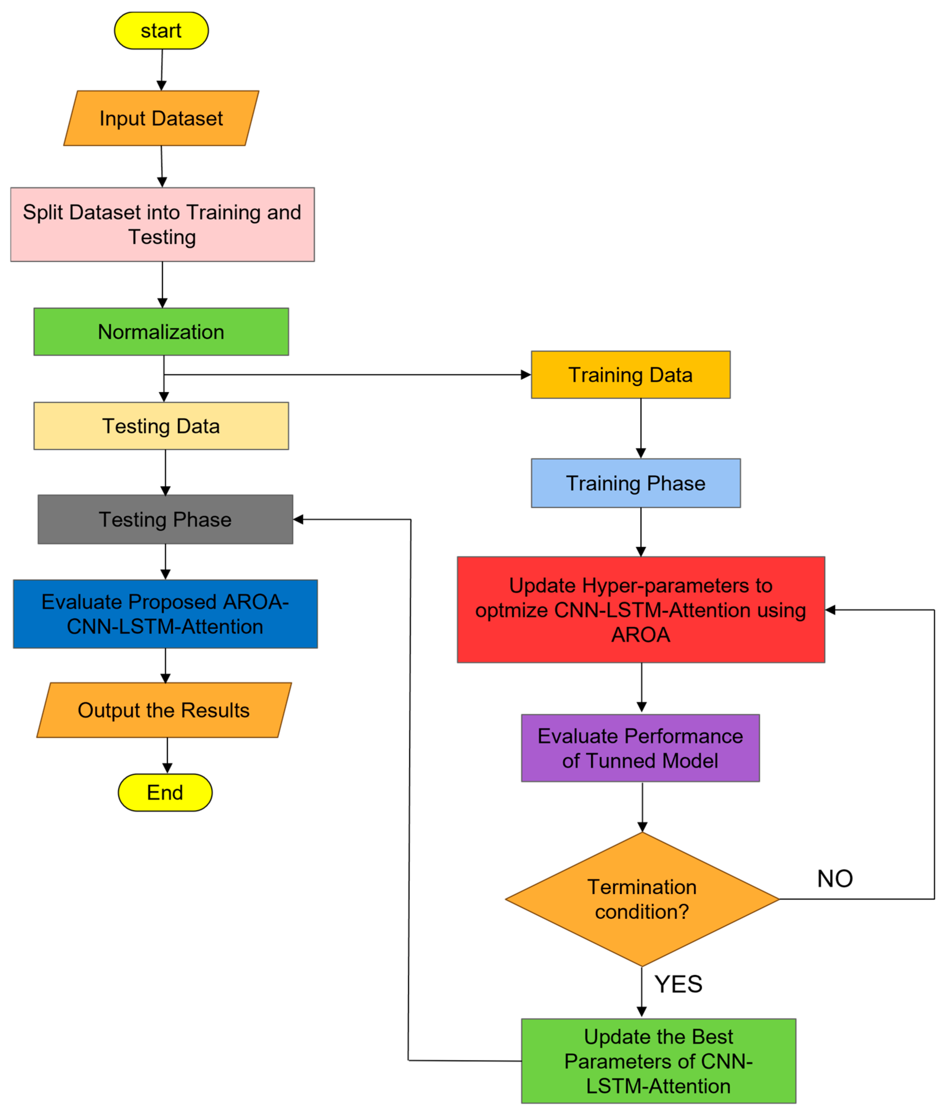
This flowchart illustrates a hybrid process that combines the adaptive rabbit optimization algorithm (AROA) with deep learning model training. On the left, the AROA begins by initializing the population and variables, balancing global exploration with local exploitation through the calculation of the dynamic energy coefficient A. When A > 1, the algorithm performs detour foraging, using adaptive step size and a global best reference mechanism to conduct an extensive search of the solution space. When A ≤ 1, it employs the differential variance strategy (DVS) to enhance local search. The algorithm then generates multiple candidate hiding locations, calculates fitness values, updates locations, and uses a memory pool mechanism to reference historical optimal solutions. This loop continues until the maximum number of iterations is reached, ultimately outputting the optimal solution.

On the right, the flowchart depicts the training process of the deep learning model. The dataset is first divided into training and test sets, after which the model is constructed and trained. The trained model then predicts the test data, and its accuracy and error are evaluated. By incorporating the AROA optimization step, hyperparameter selection and initial model conditions are optimized, enhancing the efficiency of the training process and improving the accuracy of the deep learning model’s predictions, as shown in Figure 1.

2.2. Sparrow Search Algorithm

The Sparrow Search Algorithm (SSA) is a swarm-intelligence-based optimization technique inspired by the foraging behavior of sparrows. SSA models the cooperative foraging and vigilance behaviors observed in sparrow groups, dividing individuals into two roles: foragers and sentinels. Foragers primarily search for the most optimal resource (representing the optimal solution), while sentinels remain vigilant to help the group avoid local optima (representing suboptimal traps). During each iteration of the algorithm, individuals continuously adjust their positions to improve the group’s overall solution. Due to its simplicity, efficiency, and adaptability, SSA is widely applied in complex function optimization, engineering design, and data mining.

2.3. Northern Goshawk Optimization

The Northern Goshawk Optimization (NGO) algorithm is an emerging swarm intelligence-based optimization technique inspired by the hunting behavior of the northern goshawk. By simulating the goshawk’s strategies—such as circling, diving, and precisely locking onto prey—NGO effectively searches for and tracks optimal solutions. Individuals in the algorithm gradually converge toward the global optimum through collaborative exploration and exploitation. With robust global search and local refinement capabilities, NGO is well-suited to solving complex nonlinear optimization problems and is widely applied in fields such as engineering optimization, pattern recognition, and machine learning. Its flexibility and efficiency make it highly effective in performance optimization.

2.4. Artificial Neural Network

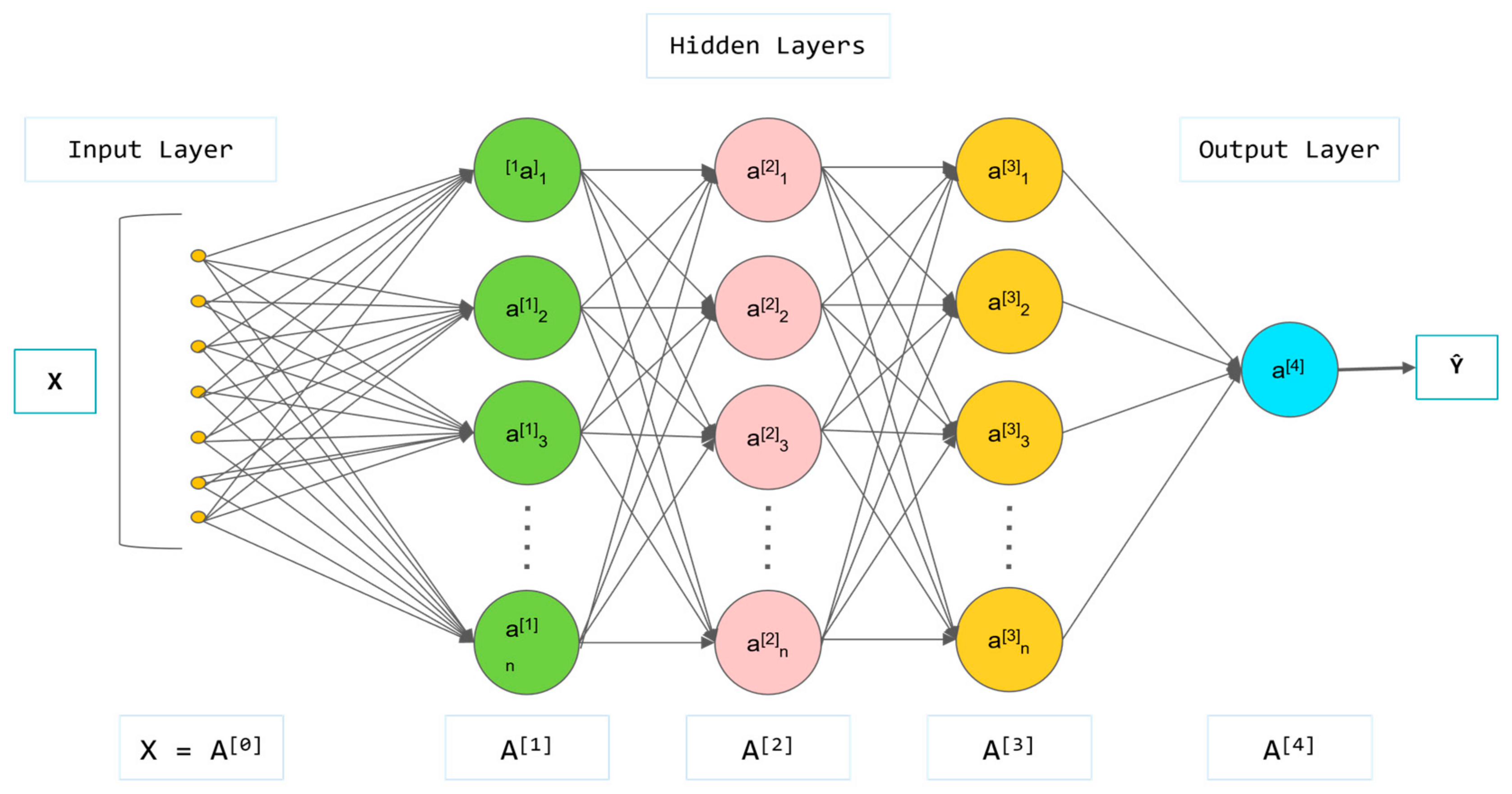
An artificial neural network (ANN) is a computational model inspired by the brain’s structure and functions, designed to process information by emulating biological neuron operations [20]. ANNs comprise multiple layers of neurons; each receives inputs, processes them, and transmits the results to subsequent layers. Neurons within these layers are interconnected via weights that regulate the input signal strength. During training, the network modifies these weights to reduce the discrepancy between the predicted and actual outputs, thereby enhancing the network’s task performance.

The fundamental working principle of an artificial neural network (ANN) is based on the interaction among neurons in each layer [21]. Initially, the input layer receives external data and forwards them to the hidden layer. Here, neurons process the data through weighted summation and activation functions to extract essential features. Subsequently, the output layer produces the network’s predicted values based on the hidden layer’s processed results. Activation functions impart nonlinear properties to the ANN, allowing it to manage complex patterns and relationships [22].

ANNs usually consist of three main components.

Input Layer: The input layer receives data from external sources, with each neuron (input node) representing a single-dimensional feature of the data. For instance, in a dataset with multiple features, each feature corresponds to one node in the input layer.

Hidden Layer: The hidden layer, situated between the input and output layers, can consist of multiple layers. Each neuron in these hidden layers connects to all the neurons in both the preceding and subsequent layers, forming a densely connected structure. Neurons in the hidden layer amalgamate information from the previous layer through weights and bias values and undergo nonlinear transformation via an activation function.

Output Layer: The output layer outputs the final computation results, with the number of nodes depending on the type of task, as illustrated in Figure 2.

2.5. LSTM Neural Network

LSTM (long short-term memory) is a specialized type of recurrent neural network (RNN) proposed by Hochreiter and Schmidhuber in 1997 to address the issue of vanishing gradients commonly encountered by standard RNNs when processing long sequential data [23]. The LSTM network possesses memory capabilities that enable it to retain long-term dependencies in sequence data, meaning that it is extensively utilized in fields such as time–series prediction, natural language processing (NLP), and speech recognition [24].

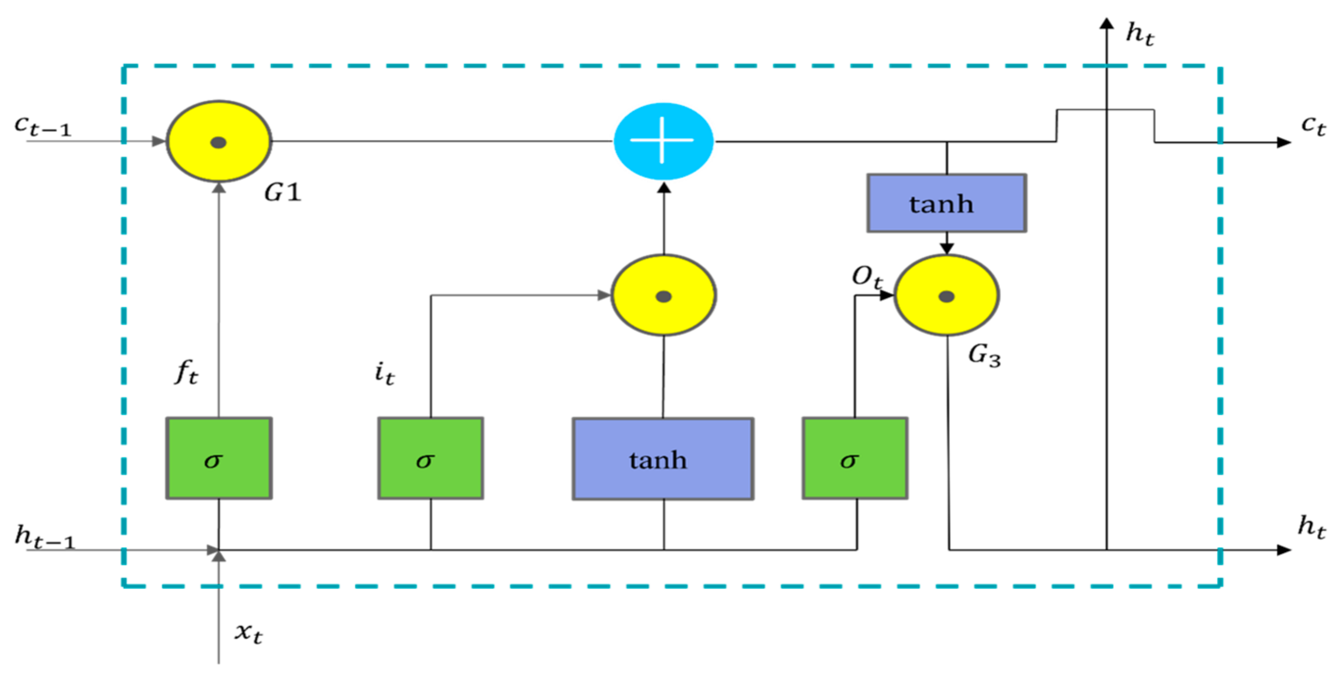
LSTM network unit: The fundamental unit of an LSTM network is the memory cell, which is regulated by several gating mechanisms that control information flow. These primarily include three core gates: the input gate, the forgetting gate, and the output gate. Through these mechanisms, the LSTM can selectively retain or discard historical information, thereby mitigating the issue of vanishing gradients.

Forgetting gate: The forgetting gate determines whether to retain the memory from the previous moment. It is governed by a sigmoid function that outputs a value between 0 and 1, where 1 signifies complete retention and 0 signifies complete discard.

$${\mathrm{f}}_{\mathrm{t}}=\mathrm{\sigma }\left({\mathrm{W}}_{\mathrm{f}}·\left[{\mathrm{h}}_{\mathrm{t}-1},{\mathrm{x}}_{\mathrm{t}}\right]+{\mathrm{b}}_{\mathrm{f}}\right)$$

(10)

where $f_t$ is the output of the forgetting gate, $h_{t-1}$ is the hidden state at the previous moment, $x_t$ is the input at the current moment, $W_f$ and $b_f$ are the weight and bias, and $\sigma$ is the Sigmoid function.

Input gate: The input gate determines whether to save new information at the current moment to the memory cell. It consists of two components: one part, using a sigmoid activation, decides which information to update; the other part, typically employing a tanh activation, generates candidate memories.

$${\mathrm{i}}_{\mathrm{t}}=\mathrm{\sigma }\left({\mathrm{W}}_{\mathrm{i}}·\left[{\mathrm{h}}_{\mathrm{t}-1},{\mathrm{x}}_{\mathrm{t}}\right]+{\mathrm{b}}_{\mathrm{i}}\right)$$

(11)

$${\tilde{\mathrm{C}}}_{\mathrm{t}}=\tan \mathrm{h}\left({\mathrm{W}}_{\mathrm{C}}·\left[{\mathrm{h}}_{\mathrm{t}-1},{\mathrm{x}}_{\mathrm{t}}\right]+{\mathrm{b}}_{\mathrm{C}}\right)$$

(12)

where $i_t$ is the output of the input gate, ${\tilde{C}}_t$ is the candidate memory value, LSTM will combine the forgetting gate and the input gate to update the memory state.

Memory state update: The memory state is updated via a forgetting gate, which determines the extent to which the previous moment’s memory should be retained, and an input gate, which assesses the impact of new information at the current moment.

$${\mathrm{C}}_{\mathrm{t}}={\mathrm{f}}_{\mathrm{t}}\ast {\mathrm{C}}_{\mathrm{t}-1}+{\mathrm{i}}_{\mathrm{t}}\ast \widetilde{{\mathrm{C}}_{\mathrm{t}}}$$

(13)

where $C_t$ is the memory state at the current moment and $C_{t-1}$ is the memory state at the previous moment.

Output gate: The output gate determines the value of the hidden state at the current moment by integrating information from the memorized state. It then outputs the hidden state through the sigmoid and tanh functions.

$${\mathrm{o}}_{\mathrm{t}}=\mathrm{\sigma }\left({\mathrm{W}}_{\mathrm{o}}·\left[{\mathrm{h}}_{\mathrm{t}-1},{\mathrm{x}}_{\mathrm{t}}\right]+{\mathrm{b}}_{\mathrm{o}}\right)$$

(14)

$${\mathrm{h}}_{\mathrm{t}}={\mathrm{o}}_{\mathrm{t}}\ast \tan \mathrm{h}\left({\mathrm{C}}_{\mathrm{t}}\right)$$

(15)

where $o_t$ is the output of the output gate and $h_t$ is the hidden state at the current moment, which is the output of the LSTM, as shown in Figure 3.

2.6. Attention Mechanism

The attention mechanism operates by focusing on the correlation between a query and a key, calculating their relationship to determine the most appropriate value. This process assigns attention weights to the value, generating the final output results [25]. The mechanism’s role within the model is primarily manifested in two areas: feature weighting and performance enhancement. The attention layer can identify and assign varying weights to input features, thereby intensifying the model’s focus on critical features, which in turn enhances prediction accuracy and robustness [26]. During the integration process, the input data are first processed through fully connected multilayers and dropout layers, and then the resultant output serves as the input to the attention layer. This layer performs a weighted summation of inputs, produces weighted features, and ultimately yields prediction results through a linear layer. Specifically, the attention mechanism improves feature selection by autonomously identifying the most crucial features for the task, enhances the model’s ability to generalize, captures long-distance dependencies in time–series or other ordered data, and, by analyzing the attention weights, allows researchers to discern which input features the model prioritizes during decision making, thus improving the model’s interpretability [27].

Calculated intermediate representation ($u_{it}$):

$${\mathrm{u}}_{\mathrm{it}}=\tan \mathrm{h}\left({\mathrm{Wx}}_{\mathrm{t}}+\mathrm{b}\right)$$

(16)

Calculating attention scores ($a_{it}$):

$${\mathrm{a}}_{\mathrm{it}}={\mathrm{u}}_{\mathrm{it}}·\mathrm{u}$$

(17)

Normalized attention score:

$${\mathrm{a}}_{\mathrm{it}}={\displaystyle \frac{\exp \left({\mathrm{a}}_{\mathrm{it}}\right)}{{{\displaystyle \sum }}_{\mathrm{k}}\exp \left({\mathrm{a}}_{\mathrm{ik}}\right)}}$$

(18)

The attention scores are normalized by the Softmax function so that they sum to the 1. weighted sum.

$$\mathrm{Output}={{\displaystyle \sum }}_{\mathrm{t}}{\mathrm{a}}_{\mathrm{it}}{\mathrm{x}}_{\mathrm{t}}$$

(19)

Attention output is obtained by weighted summation of input features using attention weights, “*” represents the weighted product operation between matrices or vectors as shown in Figure 4.

2.7. CNN

CNNs are a class of architectures prevalent in various feed-forward neural networks, primarily consisting of convolutional, pooling, and fully connected layers. These networks are especially effective for processing data with spatial structures, such as images and time–series data. CNNs efficiently process and analyze data in Euclidean space through convolutional operations, thereby demonstrating significant advantages in time–series prediction tasks [28].

The convolutional layers of CNN effectively capture local features in time–series data, utilizing mechanisms such as weight sharing and spatial invariance to improve the efficiency and accuracy of data processing. Furthermore, the pooling layer simplifies data complexity and mitigates the risk of model overfitting by implementing dimensionality reduction operations; common methods include average pooling and maximum pooling [29]. The fully connected layer incorporates these local features and maps them to the output space for subsequent classification or regression tasks after the convolutional and pooling layers have processed them.

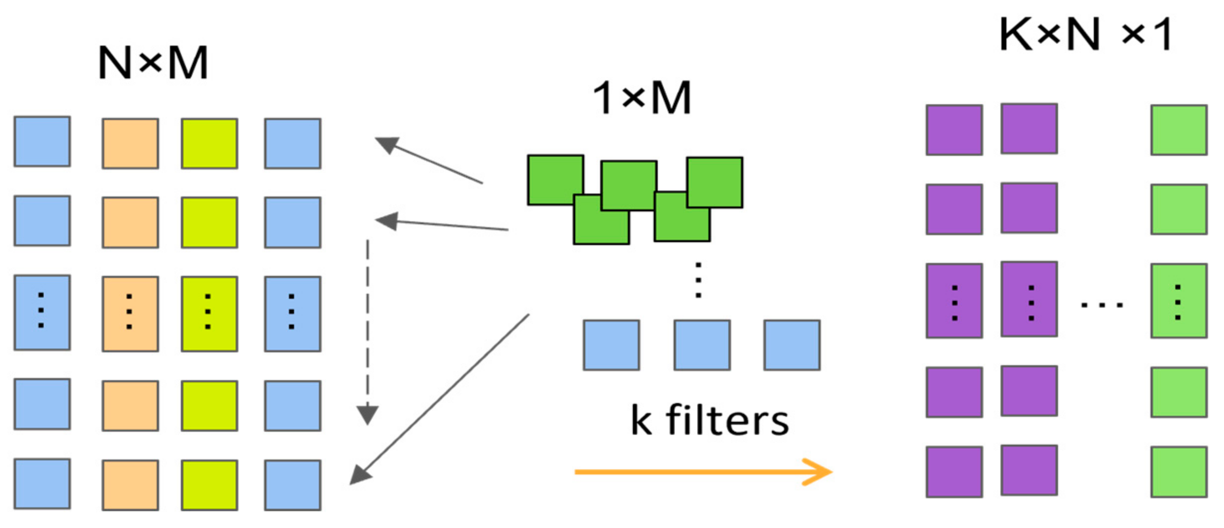
In this study, we utilize a one-dimensional convolutional neural network (1D CNN) equipped with specialized convolutional kernels to predict time–series data. This network is optimized to detect short-term pattern features in time–series, streamlining the computational demands of the model by minimizing the number of required parameters through a parameter-sharing mechanism [30]. This strategy not only boosts the model’s training efficiency but also its scalability for handling large-scale data. With this method, 1D CNNs are capable of predicting time–series data more effectively and adapting to rapidly evolving trends and patterns, as illustrated in Figure 5.

2.8. Arc Sag Prediction Model

The target variable is frequently impacted by a variety of external factors in time–series forecasting. For example, current, voltage, and temperature are all factors that can affect arc sag data. The use of correlated variables as model inputs is predicated on these correlations. The single input–single output target-variable model, the multiple input–multiple output correlated-variable and target-variable model, and the multiple input–single output correlated-variable and single-target-variable model are among the numerous approaches that can be implemented when developing an input–output prediction model. This paper proposes a novel time–series forecasting method, the multi-correlated target variable forecasting model, that incorporates the benefits of these three models to fully leverage multivariate time–series data for forecasting.

The model takes as input the target variable along with its associated multidimensional time–series. In arc droop prediction, the input data include not only the historical arc droop values but also other influencing factors, such as current, voltage, and temperature. The model’s output is the predicted future value of the target variable, specifically the arc droop.

In multistep time–series forecasting, commonly employed strategies include direct multistep forecasting and recursive multistep forecasting. Direct multistep forecasting allows for the simultaneous generation of predicted values for the target variable at multiple time points. However, this method may restrict the correlation among neighboring predicted values. Consequently, we utilize a recursive multistep forecasting approach that incrementally generates predictions for the next arc–pendant step in a rolling fashion. It is important to note that this approach can lead to the accumulation of prediction errors, which may render the predictions insignificant if the error surpasses a certain threshold. Figure 6 illustrates a multiple correlated target variable prediction model using a recursive multistep prediction strategy. In this model, Ri represents the multiple inputs from the correlated variables, O represents the input of the target variable, and assuming a step size of m, the target variable at the m + 1st data point can be predicted.

Initially, the parameters that necessitated optimization, including hyperparameters and network structure parameters, were identified in order to achieve optimal experimental results. A fitness function was subsequently created to evaluate the model’s performance under specific parameter configurations. Random combinations within a predetermined range were employed to establish the initial parameters. The model was trained and analyzed under a variety of parameter configurations to determine the fitness values of each potential solution.

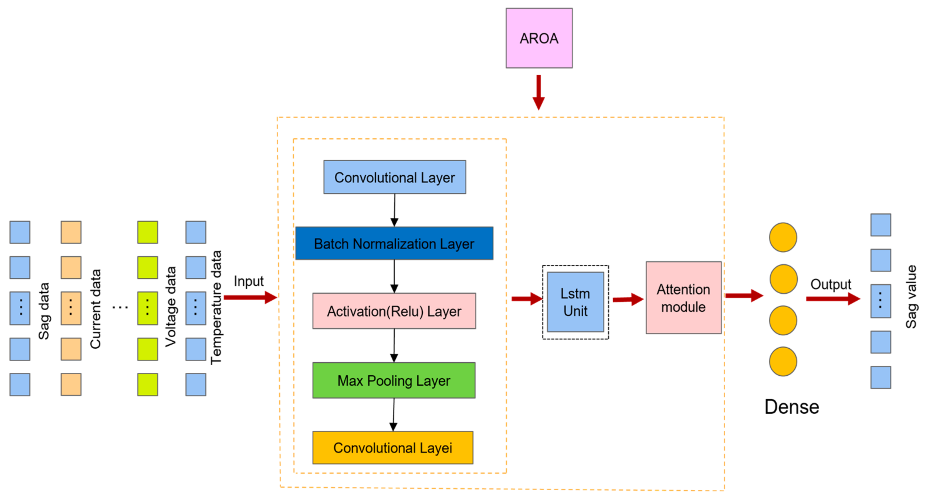
In summary, the proposed arc droop prediction model, known as the CLA model (CNN–LSTM–Attention), enables accurate forecasting of arc droop in power transmission lines under complex environmental conditions. The model begins by extracting key features from input data—such as temperature, humidity, and wind speed—using a convolutional neural network (CNN). The CNN captures local spatial information, establishing correlations between environmental factors and arc droop trends. Next, the model utilizes a long short-term memory (LSTM) network to process time–series features, effectively modeling the temporal dependencies of arc droop and incorporating historical information that influences future trends. To further enhance prediction accuracy, an attention mechanism is applied to weight the LSTM output, allowing the model to focus on key time points with greater predictive impact, thereby improving its ability to capture future arc droop trends. For hyperparameter optimization, the model incorporates the adaptive rabbit optimization algorithm (AROA), which optimizes critical hyperparameters such as convolutional kernel size, LSTM layers, neuron count per layer, and learning rate. By dynamically adjusting individual positions, the AROA balances global exploration with local exploitation, enhancing search efficiency. Its dynamic energy coefficients and differential variation strategies make AROA adaptable to complex optimization challenges, accelerating convergence speed, and improving global solution stability. The model is trained using the mean square error (MSE) as a loss function, measuring differences between predicted and actual values, and the Adam optimizer, known for stability and rapid convergence in high-dimensional spaces. To prevent overfitting, an early stopping strategy is employed, halting training if validation performance does not improve within a specified number of iterations. Model performance is evaluated using metrics such as root mean square error (RMSE) and mean absolute error (MAE), confirming its predictive accuracy and generalization capabilities. Testing results demonstrate that the model effectively forecasts arc droop trends, adapting to environmental changes and offering reliable support for real-time monitoring and early warning in power transmission. With this model, the power system can better predict and manage arc sag, enhancing transmission line safety and stability, as illustrated in Figure 7.

3. Results

3.1. Data Collection

In this study, the proposed model, AROA-CLA (AROA-CNN–LSTM–Attention), is evaluated using a dataset generated from transmission line arc sag features in a specific region. This dataset includes hourly real-time monitored climate and transmission line arc sag data for the period from 2021 to 2022, used as a case study. It comprises various parameters related to transmission lines, including voltage, temperature, conductor type, conductor tension, tower height, line length, wind speed, wind direction, and ambient humidity, as shown in the table. Together, these parameters capture the influence of transmission line operating conditions and external environmental factors on arc sag, thereby enhancing the accuracy of arc sag predictions under different weather and load conditions. Details of each dataset’s time range, data volume, scale, and model operating environment are provided, as shown in

Table 1. Data sheet.

Voltage (kV)	Temperature (°C)	Wire Type	Tension (N)	Tower Height (m)	Line Length (km)	Wind Speed (m/s)	Wind Direction (°)	Humidity (%)	Arc Droop (m)
500	−19.6	Steel-cored aluminum stranded wire	5334.22	35	13.94	4.84	338.18	72.79	3.75
500	−20.6	Steel-cored aluminum stranded wire	5062.03	35	13.94	6.25	340.38	71.79	4.41
500	−19.7	Steel-cored aluminum stranded wire	4704.50	35	13.94	6.73	338.13	72.79	5.06
500	−19.4	Steel-cored aluminum stranded wire	5177.21	35	13.94	2.88	320.68	73.79	5.67
500	−19.8	Steel-cored aluminum stranded wire	5353.28	35	13.94	6.05	312.18	73.69	6.24

and

Table 2. Information about the environment in which the data are running.

Feature	Value
Training data (80%)	1 January 2021 to 31 August 2022
Testing data (20%)	1 September 2022 to 31 December 2022
Vector length	10
Sampling rate	1 h
Numerical environment	Python 3.9.0
Libraries	Numpy: 1.26.0, TensorFlow: 2.18.0, Pandas: 2.1.1, Matplotlib: 3.8.0, Keras: 3.6.0, cuda: 12.3
Machine information	AMD Ryzen™ 9 5900HX @ 3.30 GHz, 64-bit operating system, x64-based processor (Advanced Micro Devices (AMD), Santa Clara, CA, USA) RTX 4070 Ti Super (NVIDIA Corporation, Santa Clara, CA, USA)

.

3.2. Data Processing

The data were normalized to remove outliers, and missing values were filled using the average arc sag values for the preceding and following hour. Due to the extensive dataset, the following illustrates the processing of the first hundred data points. Initially, the raw arc sag data were visualized, revealing some outliers (e.g., data points exceeding 6 m), as shown in Figure 1, which may have been caused by noise or measurement errors. During data processing, all arc sag values exceeding 6 m were treated as outliers and removed. These outliers were replaced with missing values to be filled in the next step, as shown in Figure 2. To maintain continuity, missing values were filled with the means of the adjacent data points, smoothing the data to better reflect the actual arc sag trend. After filling missing values, the data exhibited fewer abnormal fluctuations and a smoother waveform. To ensure data consistency, the arc sag values were normalized to a distribution with a mean of 0 and a standard deviation of 1. This normalization preserved the relative size of the data points while making the values more suitable for statistical analysis and machine learning modeling, as shown in Figure 8, Figure 9 and Figure 10.

3.3. Objective Function and Assessment Indicators

The model’s performance in this experiment is evaluated using a variety of metrics, such as the coefficient of determination (R²), mean absolute error (MAE), root mean square error (RMSE), and median absolute error (MedAE). The predictive accuracy and robustness of the model are assessed from a variety of perspectives using these metrics. A more exhaustive evaluation of these indicators enables a more thorough evaluation of the model’s performance and establishes a firm foundation for its optimization.

RMSE (root mean square error) measures the magnitude of the difference between predicted and actual observations. It is calculated by taking the square root of the average squared differences between predicted and actual values. A lower RMSE indicates that the model’s predictions are closer to the actual results.

$$\mathrm{RMSE}=\sqrt{{\displaystyle \frac{1}{\mathrm{n}}}{{\displaystyle \sum }}_{\mathrm{i}=1}^{\mathrm{n}}{\left({\hat{\mathrm{y}}}_{\mathrm{i}}-{\mathrm{y}}_{\mathrm{i}}\right)}^2}$$

(20)

MAE (mean absolute error) measures the average absolute difference between predicted and actual values, assessing the accuracy of the model’s predictions. A lower MAE value indicates that the model’s predictions are closer to the actual values.

$$\mathrm{MAE}={\displaystyle \frac{1}{\mathrm{n}}}{{\displaystyle \sum }}_{\mathrm{i}=1}^{\mathrm{n}}\left|{\hat{\mathrm{y}}}_{\mathrm{i}}-{\mathrm{y}}_{\mathrm{i}}\right|$$

(21)

R² (coefficient of determination) assesses how well the model fits the data, with values ranging from 0 to 1. An R² value closer to 1 indicates that a larger proportion of variance in the observed data is explained by the model, signifying greater predictive power.

$${\mathrm{R}}^2=1-{\displaystyle \frac{{{\displaystyle \sum }}_{\mathrm{i}=1}^{\mathrm{n}}{\left({\hat{\mathrm{y}}}_{\mathrm{i}}-{\mathrm{y}}_{\mathrm{i}}\right)}^2}{{{\displaystyle \sum }}_{\mathrm{i}=1}^{\mathrm{n}}{\left({\mathrm{y}}_{\mathrm{i}}-\stackrel{-}{\mathrm{y}}\right)}^2}}$$

(22)

MedAE is a metric that is employed to evaluate the predictive accuracy of a model. It assesses the predictive performance by determining the median of the absolute differences between the predicted and actual values. MedAE is particularly effective in datasets with outliers, as it is significantly insensitive to outliers due to its dependence on the median. This attribute enables MedAE to more precisely represent the model’s typical prediction error. A reduced MedAE value suggests that the model’s predictions are more closely aligned with the actual outcomes, indicating improved model performance. This metric is particularly well-suited for situations in which it is essential to mitigate the impact of outliers.

$$\mathrm{MedAE}=\mathrm{median}\left(\left|{\hat{\mathrm{y}}}_{\mathrm{i}}-{\mathrm{y}}_{\mathrm{i}}\right|\right)$$

(23)

The training and testing process of the prediction model proposed in this paper is illustrated in Figure 11. Initially, the dataset is partitioned into training and testing sets in an 8:2 ratio, and the data are normalized to guarantee a consistent feature scale. The adaptive rabbit optimization algorithm (AROA) generates new candidate solutions through iteration during the training phase. It then evaluates the fitness value of each candidate solution using the fitness function and conducts a global search to identify the optimal parameter configuration. Afterward, it ascertains whether the termination condition is satisfied by either the optimal fitness value or the specified maximum number of iterations. AROA will continue to optimize the hyperparameters of the CLA model if the condition is not satisfied. The optimal parameters of the CLA model will be determined if the termination condition is satisfied. In the testing phase, the CLA model is further optimized using the LSTM global optimal solution derived by AROA. The efficacy of the CLA model on the test set is subsequently evaluated using these optimized parameters.

3.4. Predictive Modeling Results and Analysis

This section evaluates the predictive performance of the AROA-CLA model by comparing it with other prevalent models used for predicting arc droop. Initially, the AROA-CLA model is compared with LSTM and CNN-LSTM models across various time steps to establish its advantages. The training details of the models are provided in

Table 3. CLA mode l parameters.

Parameters		Details
	Filter	32
	Kernel size	2
Conv1D	Activation	ReLu
	Kernel regularizer	L2 (strength 0.1)
MaxPooling1D	pool size	2
Dropout	Dropout Rate	0.4
LSTM	Units1	10
	Units2	10
Attention	Units	20
	Unites	10
Dense1	Activation	ReLu
Dense2	unites	1

. The evaluation encompasses different periods, including high temperatures (noon to afternoon), low temperatures (early morning and night), and extreme weather or peak loads, to effectively capture the cyclical natural features in the data. For comparison, 1 h and whole time steps are used. The whole time step aids in forecasting bi-daily trends and identifying long-term, slow-varying factors influencing arc sag. Conversely, the 1 h time step focuses on hourly forecasts, quickly capturing rapid changes and promptly identifying sudden shifts.

In

Table 4. Performance of the model at 1 time step.

	${\mathbf{R}}^2$	RMSE (cm)	MAE (cm)	MedAE (cm)
CLA	0.878	86.8	78.5	18.7
CNN-LSTM	0.768	127.4	101.9	36.7
LSTM–Attention	0.773	134.1	106.7	40.13
CNN–Attention	0.689	122.7	100.5	32.47
LSTM	0.581	231.4	183.4	58.6

and

Table 5. Performance of the model at whole time steps.

	${\mathbf{R}}^2$	RMSE (cm)	MAE (cm)	MedAE (cm)
CLA	0.898	68.1	63.5	18.7
CNN-LSTM	0.738	104.6	107.9	29.7
LSTM–Attention	0.718	114.1	106.3	32.8
CNN–Attention	0.720	108.7	92.4	31.7
LSTM	0.681	267.4	201.4	59.6

, the RMSE, MAE, R², and MedAE scores of the CLA, LSTM, and CNN-LSTM models at 1 and whole time steps are presented. Higher R² values and lower RMSE and MAE values indicate improved model performance, while lower MedAE values indicate higher resilience to data perturbations. The models’ ability to predict arc sag is illustrated in Figure 12 and Figure 13, which provide statistics on transmission line parameters and arc sag data from 2021 to 2022.

The CNN-LSTM model substantially outperforms the LSTM model in all four performance metrics at a 1 time step interval, thereby illustrating its superior capacity to extract spatiotemporal features from the arc droop parameters. The CLA method results in a R² score of 0.878, an RMSE of 86.8, an MAE of 78.5, and a MedAE of 18.7. This indicates that the CLA method not only outperforms the CNN-LSTM and LSTM models, but also has the highest resistance to interference. In particular, the R² scores demonstrate advances of 0.116 and 0.273 compared to the CNN-LSTM and LSTM models, respectively. Additionally, the RMSE, MAE, and MedAE values demonstrate exceptional performance. At a whole time step interval, the CLA model’s R² score increases to 0.898, while the RMSE decreases to 68.1, the MAE to 63.5, and the MedAE remains at 18.7. This indicates a 0.16 and 0.217 increase in R² compared to the CNN-LSTM and LSTM models, respectively. The improvements in RMSE, MAE, and MedAE are more noticeable. The R² scores of 0.878 and 0.898, respectively, are indicative of high predictive stability when comparing the 1- and whole time step intervals. This comparison emphasizes that the CLA model demonstrates superior adaptability and stability across a variety of time scales, whereas the training outcomes of general models are influenced by the time step value. The performance benefits of the attention mechanism within the CLA model are accentuated by the extended time step of whole, which effectively concentrates on the most critical components of historical data for future power prediction, thereby substantially increasing prediction accuracy.

The AROA algorithm is implemented by the AROA-CLA model to optimize four LSTM parameters: network units, regularization term, learning rate, and an unspecified parameter. Before optimization can commence, initial parameters are established for AROA training. The search for the global optimal solution is preceded by the updating of individual fitness in accordance with policy. Figure 10 depicts the optimization process across 50 iterations,

Table 6. AROA parameter settings and optimization ranges.

	Parameters	Details
	Pop	3
	MaxIter	50
	Dim	4
	LSTM units1	[32, 128]
Best parameters	LSTM regularizer	[0.001, 0.01]
	LSTM units2	[32, 64]
	Learning rate	[0.001, 0.01]

outlines the AROA parameters, and Figure 14 and Figure 15 display the training and testing losses throughout 100 iterations.

By the sixth iteration, the AROA optimization process obtains a fitness value of 0.009, as illustrated in Figure 14, suggesting swift convergence. It defines optimal fitness and determines four globally optimal parameters for the LSTM by the 16th iteration. The first layer contains 83 units with a regularization factor of 1.627 × 10⁻⁷, and the second layer contains 58 units with a learning rate of 0.00032. The CLA model was trained and evaluated on the arc droop dataset using these parameters. As illustrated in Figure 15, the loss profiles for both the training and testing phases are virtually identical, indicating a high level of consistency between the two. The loss function decreases rapidly during the first iteration and stabilizes by the 19th iteration, with a loss value below 0.02. This result demonstrates the effectiveness of the AROA algorithm in enhancing model robustness, optimizing algorithm design, efficiently absorbing information, and accelerating convergence. This analysis corroborates the AROA algorithm’s efficacy and superiority in optimizing model parameters. Next, comparisons will be made with other optimization algorithms and prediction models, specifically the SSA Sparrow Optimization Algorithm, the Northern Goshawk Optimization Algorithm, and the ANN model. The SSA-CLA (SSA–CNN–LSTM–Attention) model combines the advantages of automated parameter optimization, efficient feature extraction and processing, key feature attention mechanisms, and multi-algorithm integration, resulting in a highly efficient, accurate, and adaptable framework. The NGO-CLA (NGO–CNN–LSTM–Attention) model constitutes a robust and flexible deep learning framework, integrating the Northern Goshawk Optimization Algorithm (NGO) for multi-objective optimization, the convolutional neural network (CNN) for spatial feature extraction, the long short-term memory (LSTM) network for handling temporal dependencies, and the attention mechanism (ATM) for enhancing focus on key features. These comparisons will further validate the effectiveness of the proposed AROA-CLA model in arc sag prediction, as shown in

Table 7. Results of different models at 1 time step.

Model	${\mathbf{R}}^2$	RMSE (cm)	MAE (cm)	MedAE (cm)
AROA-CLA	0.974	28.5	23.3	8.7
SSA-CLA	0.934	32.6	28.7	9.1
NGO-CLA	0.947	37.4	31.4	11.1
ANN	0.867	75.1	68.4	15.3
CLA	0.878	86.8	78.5	18.7
LSTM	0.581	231.4	183.4	58.6
CNN-LSTM	0.768	127.4	101.9	36.7

and

Table 8. Results of different models at whole time steps.

Model	${\mathbf{R}}^2$	RMSE (cm)	MAE (cm)	MedAE (cm)
AROA-CLA	0.982	27.4	24.5	7.7
SSA-CLA	0.949	29.7	28.4	10.8
NGO-CLA	0.946	34.7	31.5	9.7
ANN	0.845	88.4	70.7	16.1
CLA	0.898	68.1	63.5	18.7
LSTM	0.681	267.4	201.4	59.6
CNN-LSTM	0.738	104.6	97.9	29.7

and Figure 16 and Figure 17.

Compared to the conventional model, the AROA–CNN–LSTM–Attention model achieves an $R^2$ score of 0.974 at step 1, which is 0.096, 0.393, and 0.206 higher than the CLA, LSTM, and CNN-LSTM models, respectively. When compared to recently developed optimization models, it outperforms the SSA-CLA and NGO-CLA models by 0.04 and 0.027, and has the lowest RMSE, MAE, and MedAE scores. For the full-time step, the AROA-CLA model attains an $R^2$ score of 0.982, surpassing the CLA, LSTM, and CNN-LSTM models by 0.084, 0.301, and 0.199, respectively. It also outperforms the SSA-CLA and NGO-CLA models by 0.033 and 0.036, achieving the lowest scores in RMSE, MAE, and MedAE, demonstrating that the AROA–CNN–LSTM–Attention model is optimal at the whole time step. This performance highlights the AROA algorithm’s ability to effectively tune the CNN–LSTM–Attention model parameters, thereby enhancing model generalization. Since the arc sag dataset from 2021–2022 was sampled at an hourly frequency, the resulting prediction curves contain numerous data points, making them difficult to display comprehensively. Therefore, the last 200 data points from the experimental tests were selected for visualization, as shown in Figure 18 and Figure 19.

4. Conclusions

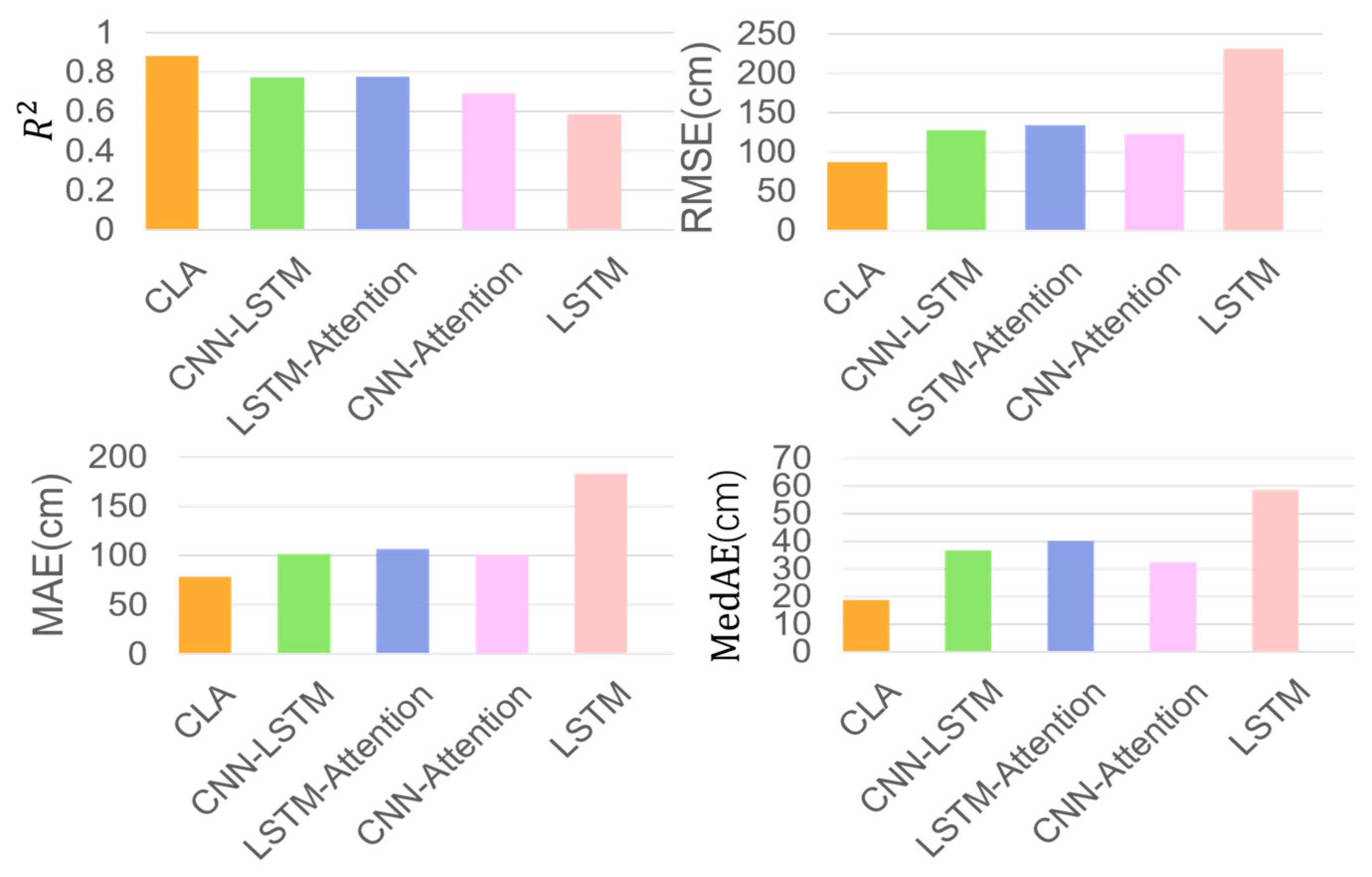
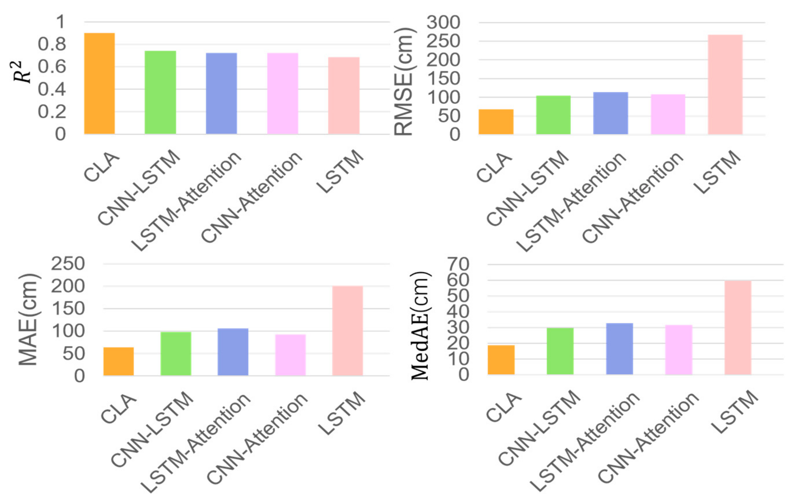
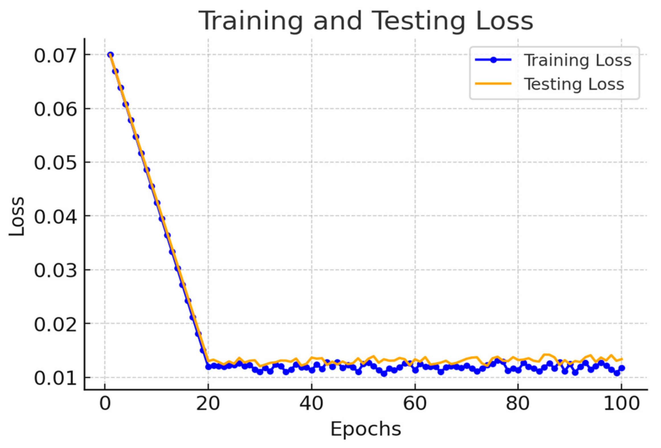
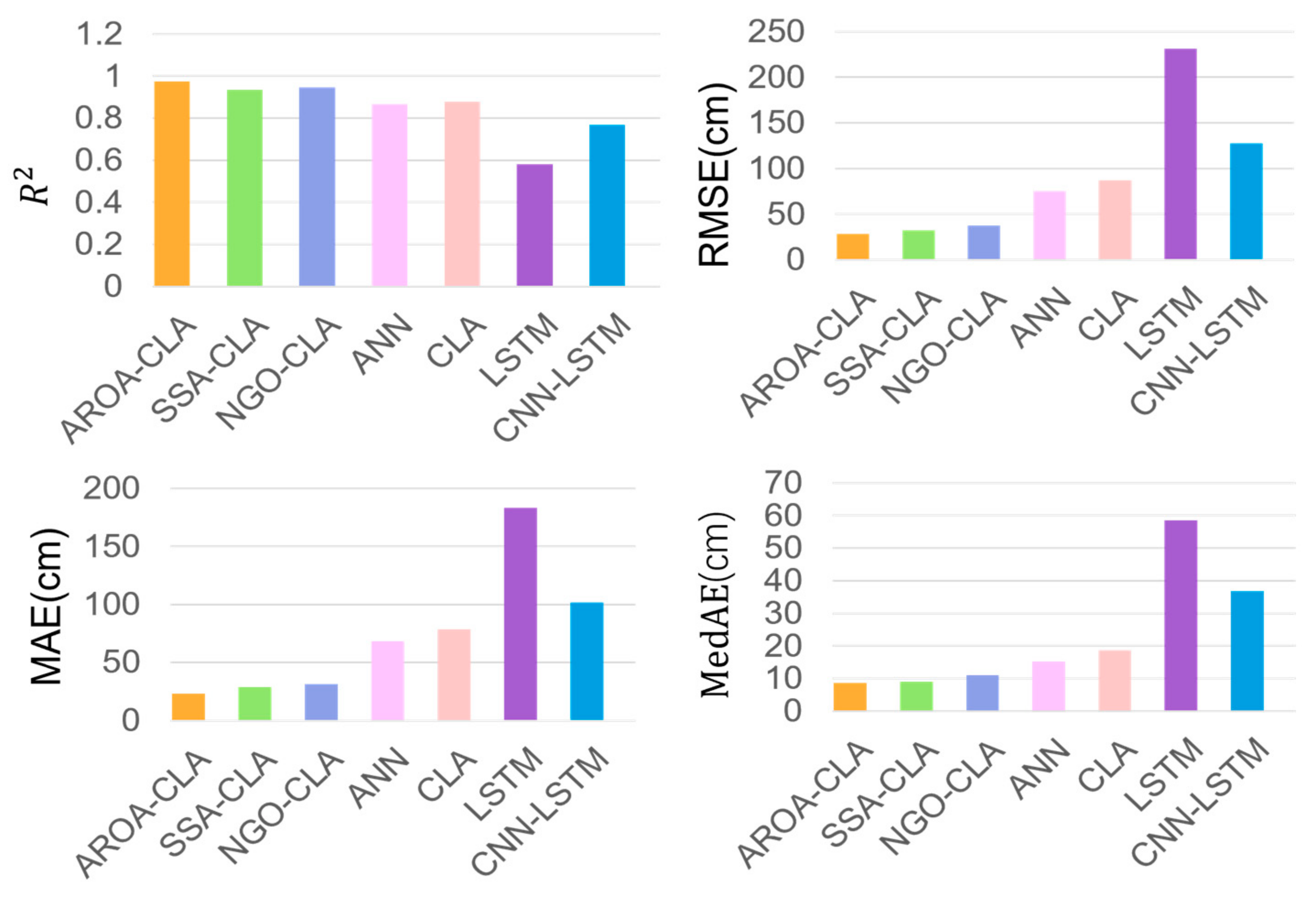
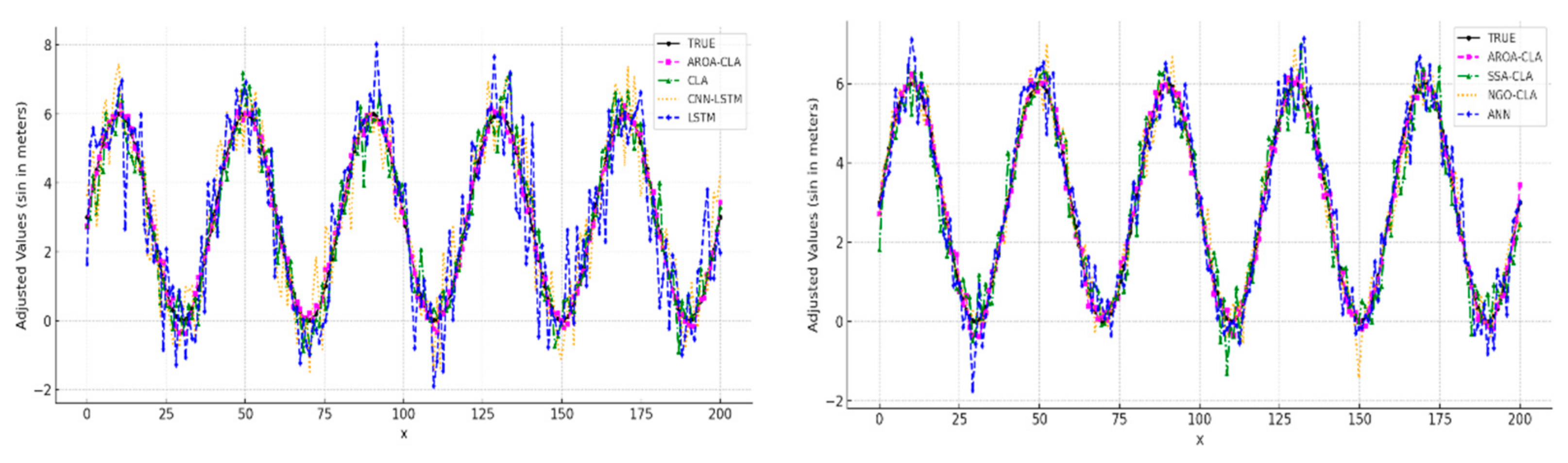
In this study, a new prediction model, AROA–CNN–LSTM–Attention (AROA-CLA), is proposed to address the challenging task of arc sag time–series prediction for transmission lines. This model integrates the Adaptive Rabbit Optimization Algorithm (AROA) into the CNN–LSTM–Attention framework, marking the first use of AROA within the CLA model for parameter optimization. This approach enhances the model’s focus on key parts of historical data and leverages advanced time–series processing capabilities to improve prediction accuracy and stability. Additionally, a multi-correlated target variable prediction model is introduced, utilizing both univariate and multivariate time–series inputs, where the target variable and associated multivariate time–series serve as model inputs. Experimental results demonstrate the model’s adaptability and stability across various time scales. The AROA algorithm performs efficiently in optimizing model parameters, reducing the loss value to below 0.01 by the sixth iteration, which significantly accelerates the model’s convergence speed. With an $R^2$ score of 0.974, the AROA-CLA model achieves the lowest RMSE, MAE, and MedAE compared to traditional methods and recently developed optimization models with a step size of whole, highlighting its superiority, stability, and resilience to perturbations. These results confirm the AROA-CLA model’s effectiveness and applicability in arc sag prediction. Furthermore, the AROA-CLA model not only achieves high prediction accuracy but also demonstrates consistent performance during both training and testing, reflecting its strong generalization ability and robustness. Future research could explore the potential and scalability of the AROA-CLA model in other application domains.