Abstract
Federated Learning (FL) revolutionizes collaborative machine learning among Internet of Things (IoT) devices by enabling them to train models collectively while preserving data privacy. FL algorithms fall into two primary categories: synchronous and asynchronous. While synchronous FL efficiently handles straggler devices, its convergence speed and model accuracy can be compromised. In contrast, asynchronous FL allows all devices to participate but incurs high communication overhead and potential model staleness. To overcome these limitations, the paper introduces a semi-synchronous FL framework that uses client tiering based on computing and communication latencies. Clients in different tiers upload their local models at distinct frequencies, striking a balance between straggler mitigation and communication costs. Building on this, the paper proposes the Dynamic client clustering, bandwidth allocation, and local training for semi-synchronous Federated learning (DecantFed) algorithm to dynamically optimize client clustering, bandwidth allocation, and local training workloads in order to maximize data sample processing rates in FL. DecantFed dynamically optimizes client clustering, bandwidth allocation, and local training workloads for maximizing data processing rates in FL. It also adapts client learning rates according to their tiers, thus addressing the model staleness issue. Extensive simulations using benchmark datasets like MNIST and CIFAR-10, under both IID and non-IID scenarios, demonstrate DecantFed’s superior performance. It outperforms FedAvg and FedProx in convergence speed and delivers at least a 28% improvement in model accuracy, compared to FedProx.
1. Introduction
With billions of connected Internet of Things (IoT) devices being deployed in our physical world, IoT data are produced in a large volume and high velocity [1]. Analyzing these IoT data streams is invaluable to various IoT applications, which can provide intelligent services to users [2]. However, most IoT data streams contain users’ personal information, and so users are not willing to share these IoT data streams with third parties but keep them locally, thus leading to data silos. To break data silos without compromising data privacy, federated learning (FL) has been proposed for enabling IoT devices to collaboratively and locally train machine learning models without sharing their data samples [3,4].
In general, there are four steps in each global iteration during the FL process: (1) Global model broadcasting, i.e., an FL server initializes a global model and broadcasts it to all the selected clients via a wireless network. (2) Local model training, i.e., each selected client trains the received global model over its local data samples to derive a local model based on, for example, stochastic gradient descent (SGD). (3) Local model update, i.e., each selected client uploads its local model to the FL server via the wireless network. (4) Global model update: the FL server aggregates all the received local models to generate a new global model for the next global iteration. The global iteration continues until the global iteration is converged. A typical example of using FL is training next-word prediction models [3] such as those used in text input systems on smartphones. In this scenario, multiple smartphones collaborate to train a shared model for predicting the next word in a message but without sharing the actual text messages or any private data with each other. Instead, the devices send only model updates to a central server, which aggregates these updates and updates the global model. This ensures that sensitive data, like the content of users’ messages, remains on the device and is not shared with others or stored centrally. Fast model training or convergence is critical as users expect quick and accurate responses, so delays in prediction accuracy or speed would result in a poor user experience. Note that in this paper, we assume that all data samples are labeled, as is common in many FL settings. While leveraging unlabeled data could potentially enhance model training and accuracy, this falls outside the scope of the current work. Future studies could explore semi-supervised or unsupervised learning approaches, such as self-training [5,6,7] or consistency regularization [8,9,10], to integrate unlabeled data and further improve model performance.
Using conventional FL, which randomly selects many clients to participate in the FL process, may lead to the straggler problem [11]. Here, stragglers refer to clients with low computational capabilities, which require more time to train models, and/or clients with low communication data rates, which, in turn, experience delays in uploading models. So, the FL server has to wait a long time for these stragglers to compute and upload their local models to the FL server, thus leading to a long training time (which equals the sum of the latency for all the global iterations). To reduce the waiting time of the FL server, two main solutions address the straggler problem: synchronous FL and asynchronous FL. (1) In synchronous FL, the FL server sets up a deadline , and so it only selects the qualified clients who can finish its local model training and upload before the deadline in order to participate in the FL process. All the local models that are received after the deadline will be discarded [12]. However, synchronous FL has its drawbacks. First, it reduces the number of participating clients, thus slowing down the convergence rate by requiring more global iterations to reach convergence [13]. Second, synchronous FL may cause model overfitting due to reduced data sample diversity. That is, the derived model can fit well for the data samples in these qualified clients but not in the non-qualified clients, thus reducing the model’s accuracy. (2) In asynchronous FL, the FL server enables all the clients to participate and updates the global model immediately upon receiving an update from any client. The updated global model is then sent only to the client, which just uploads its local model [14]. Asynchronous FL can reduce the waiting time of the FL server, but it faces two key challenges: (i) The high communication cost, as both the server and clients frequently exchange models; (ii) The model stale problem where slower clients are trained on outdated global models, leading to a reduction in the convergence rate [15,16,17].
To address the limitations of both synchronous and asynchronous FL, we propose semi-synchronous FL. In this method, all clients in the system are grouped into different tiers based on the deadline of a global iteration, denoted as , and the clients’ model training and uploading latency. Specifically, if a client can complete model training and uploading within the interval of and , it is assigned to the tier. As illustrated in Figure 1, consider an example where Client-1 and Client-2 complete their model training and upload before the deadline , thus being assigned to the 1st tier, which has a deadline of . On the other hand, Client-3 completes its local model training and uploading between and , placing it in the 2nd tier with a deadline of . These different tiers indicate that clients upload their local models to the FL server at varying frequencies. For example, the upload frequency of Client-1 and Client-2 is twice as high as that of Client-3.
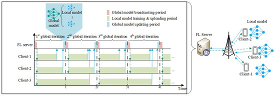
Figure 1.
The semi-synchronous FL framework.
Semi-synchronous FL differs from synchronous FL since all the clients participate in the training process to increase the diversity of training samples, avoid model overfitting and stragglers, and reduce the convergence time. Semi-synchronous FL also differs from asynchronous FL since different clients in semi-synchronous FL have to follow their own schedules in order to upload their local models, while the FL server still has to wait for a global iteration to terminate in order to aggregate the received local models, which reduces the communication cost and mitigates the model stale problem found in asynchronous FL.
Although semi-synchronous FL can potentially resolve the drawbacks of synchronous and asynchronous FL, it has its own unveiled challenges. First: how to cluster clients into different tiers? Client clustering depends on the model training and uploading latency of a client. However, it is not easy to estimate the uploading latency of a client, which, for example, depends on the number of clients in this tier. In particular, more clients in the tier sharing the bandwidth resource leads to higher uploading latency and vice versa. Hence, it is hard to estimate the uploading latency if client clustering has not been determined. Second: how to dynamically assign computing workloads to different clients? In conventional FL, clients perform uniform local training, meaning that clients train their local models based on the same number of data samples. This results in high-computing-capacity clients having long idle time in each global iteration. For example, as shown in Figure 1, Client-1 in tier-1 has a high computing capacity to quickly finish its local model training, upload its local model to the FL server, and then wait for the beginning of a new global iteration. Instead of waiting, Client-1 can train more data samples to generate a better local model. Studies have demonstrated that training more data samples per client can accelerate model convergence in FL [18,19,20]. Thus, dynamically optimizing the training workload of a client based on its computing capacity can potentially improve the FL performance. However, workload optimization and client clustering are coupled together since a different workload (i.e., selecting a different number of data samples to train the model) of a client would change its model computing and uploading latency, which leads to a different client clustering. The paper aims to resolve the mentioned two challenges by jointly optimizing client clustering, bandwidth allocation, and workload assignment in the context of semi-synchronous FL. The main contributions of the paper are summarized as follows.
- We propose semi-synchronous FL to resolve the drawbacks of synchronous and asynchronous FL.
- We propose dynamic workload optimization in semi-synchronous FL and prove that dynamic workload optimization outperforms uniform local training in semi-synchronous FL via extensive simulations.
- To resolve the challenges in semi-synchronous FL, we formulate an optimization problem and design Dynamic client clustering, bandwidth allocation, and workload optimization for semi-synchronous Federated learning (DecantFed) algorithm to solve the problem.
The rest of the paper is organized as follows. The related work is summarized in Section 2. The system models and the problem formulation are presented in Section 3. Section 4 describes the proposed DecantFed algorithm to efficiently solve the problem. Simulation results are provided and analyzed in Section 5, and we conclude the paper in Section 6.
2. Related Work
To solve the straggler problem in FL, synchronous FL has been proposed to set up a deadline and discard the local models received after the deadline. Since having more clients uploading their models can potentially accelerate the training speed, Nishio et al. [14] proposed to select the maximum number of clients who can upload their local models before the deadline. Lee et al. [21] designed a mobile device performance-disparity-aware mechanism to adaptatively adjust the deadline. On the other hand, since the latency of a client in uploading its model depends on the allocated bandwidth, wireless resource management and client selection are usually optimized jointly. For example, Albaseer et al. [19] aimed to jointly optimize the bandwidth allocation and client selection such that the weighted number of the selected clients is maximized. Given a set of selected clients, Li et al. [20] proposed that FedProx assign more local epochs to clients with high computing capacity, where more local epochs imply a higher computing workload. FedProx can potentially reduce the number of global iterations but may hurt the global model convergence owing to local model overfitting, especially when a data sample distribution is non-independent and identically distributed (non-IID) [22]. FedProx adds a proximal term in the loss function for each client’s local model to mitigate the local model overfitting problem. Albelaihi et al. [12] considered time division multiple access (TDMA) as the wireless resource-sharing approach in wireless FL. While TDMA can enhance bandwidth utilization, it can also lead to a waiting period for the selected client to upload their local model due to the wireless channel’s limited availability. To account for the potential impact of waiting time on client selection, a heuristic algorithm is developed to maximize the number of selected clients who can upload their models before the deadline. Selecting more clients to participate in each global iteration leads to the high energy consumption of the clients [23], and so Yu et al. [24] designed a solution to maximize the tradeoff between the total energy consumption of the selected clients and the number of the selected clients in each global iteration. Instead of maximizing the number of selected clients in each global iteration, Xu and Wang [25] proposed that increasing the number of the selected clients over global iterations would have a faster convergence rate. Based on this hypothesis, they designed a long-term client selection and bandwidth allocation solution, which aims to maximize the weighted total number of the selected clients for all the global iterations while satisfying the energy budget of the clients and bandwidth capacity limitation. Here, the weight is increasing over the global iterations.
Instead of waiting for the deadline to expire before updating the global model in synchronous FL, asynchronous FL allows the FL server to immediately update the global model once it receives a local model [15,26,27]. However, as we mentioned before, asynchronous FL has the model stale problem, i.e., the slower clients may train their local models based on an outdated global model, which results in slow convergence or even leads to model divergence [28,29]. To mitigate the model stale problem, Xie et al. [30] proposed a new global model aggregation, where the new global model equals the weighted sum of the old global model and the received local model. Here, the weight of a local model is a function of the local model staleness, i.e., a longer delay of training and uploading a local model for a client leads to a higher staleness of the local model and a lower weight of the local model. Chen et al. [31] proposed the asynchronous online FL method, where different clients collaboratively train a global model over continuous data streams locally. The FL server updates the global model once it receives the gradient, learning rate, and the number of data samples from a client. Another drawback of asynchronous FL is the high communication cost, especially for faster clients since they more frequently exchange their models with the FL server. A potential solution could be to enable the FL server to update the global model after it receives a number of local models instead of receiving each local model. The concept of client clustering has been proposed to mitigate model accuracy reduction caused by non-IID data. For example, Christopher [32] suggested clustering clients based on the similarity of their local updates to the global model. The clients within the same cluster are trained independently and in parallel on a specialized model. Similarly, Kim et al. [33] proposed a customized generative adversarial network for grouping clients into clusters without sharing raw data. Based on that, they also developed heuristic algorithms to dynamically adjust cluster numbers and client associations based on loss function values. While clustering reduces the impact of non-IID data, these methods overlook differences in client capacities, leaving the straggler problem unresolved.
3. System Models and Problem Formulation
In this section, we will provide the related system models and formulate the problem for jointly optimizing client clustering, bandwidth allocation, and workload optimization in semi-synchronous wireless FL. Denote the set of clients in the system as ; i is used to index these clients. All the clients in will be clustered into different tiers and will upload their local models to the FL server via a base station (BS). Denote the set of tiers as ; j is used to index these tiers. In our scenario, we consider frequency division multiple access (FDMA) as the wireless resource-sharing mechanism among various tiers. This implies that each tier will be allotted a distinct frequency band that does not overlap with other tiers, and the bandwidth allocated to each tier will be optimized. Let be the bandwidth allocated to tier j. In addition, the clients within the same tier would share the same frequency band based on TDMA, meaning that the clients would take turns acquiring the entire frequency band to upload their models. As mentioned in Section II, TDMA may introduce extra waiting time for a client to wait for wireless bandwidth to be available. Therefore, if client i is in tier j, then the latency of client i in training and uploading its local model to the FL server is
where is the computing latency of client i in training its local model, is the delay of client i in tier j to wait for the frequency band to be available, and is the uploading latency of client i in tier j to upload its local model.
3.1. Computing Latency
The computing latency of client i can be estimated by [34]
where is the number of CPU cycles required for training a sample of its local model, is the number of samples to be trained on client i; and is the CPU frequency of client i.
3.2. Uploading Latency
According to [35,36,37], the achievable data rate of client i in tier j can be estimated by where is the amount of bandwidth allocated to clients in tier j, is the transmission power density of client i, is the channel gain from client i to the BS, and is the average background noise. Note that the algorithm proposed in Section 4 does not rely on this equation for calculating the client’s upload data rate. Other, more sophisticated models that provide better estimates for upload data rates can be easily integrated into our algorithm to enhance its performance. Consequently, the latency of client i in tier j to upload its local model with size of s to the BS is .
3.3. Waiting Time
Once client i finishes its local model training, it can immediately upload its local model to the FL server if the bandwidth is unoccupied, i.e., there is no other client currently uploading its local model. However, if the bandwidth is occupied, client i has to wait, and the waiting time depends on its position in the queue. Specifically, let denote the set of clients in tier j, who are sorted based on the increasing order of their computing latency, i.e., , , where is the index of the clients in . Hence, if client i is in tier j, its waiting time can be calculated based on the following recursive function.
3.4. Problem Formulation
Assuming the FL server can access the state information of all clients, including their channel gains, CPU frequencies, and transmission power, and that all clients are time-synchronized and cooperative, adhering to the clustering, workload, and bandwidth allocations provided by the FL server. We formulate the problem to jointly optimize client clustering, bandwidth allocation, and workload management in semi-synchronous FL as follows.
where is a binary variable to indicate if client i is clustered in tier j (i.e., ) or not (i.e., ), , is the workload allocation in terms of the number of data samples being used to train local models for all the clients, implies the amount of bandwidth allocated to different tiers, and indicates the frequency of the clients in tier j uploading their local models. i.e., . Here, indicates the last tier. Hence, a larger means tier j is a lower tier, and clients in this tier upload their local models more frequently. Training a model over more data samples leads to higher model accuracy. Based on this intuition, we set up the objective of so that the number of training data samples per unit time is maximized, where is the frequency of client i in uploading its local model, and is the number of data samples used to train its local model. Constraint (5) indicates the clients in different tiers should meet their tier deadlines. Constraint (6) defines the minimum number of the samples, denoted as , to be trained locally by each client. Constraint (7) specifies each client should only be clustered into exactly one tier. Constraint (8) refers to being a binary variable, and Constraint (9) means the amount of bandwidth allocated to all the tiers no larger than B, where B is the available bandwidth at the BS.
4. The DecantFed Algorithm
is difficult to solve. First, client clustering , bandwidth allocation , and workload management are coupled together. For instance, allocating less bandwidth or selecting more data samples for client i in a tier would increase its uploading latency and computing latency , thus leading to client i being unable to upload its local model before its tier deadline. As a result, client i has to be assigned to the next tier, which has a longer tier deadline. We propose DecantFed to efficiently solve problem . The basic idea of DecantFed is to decompose into two sub-problems and solve them individually.
4.1. Client Clustering and Bandwidth Allocation
Assume that each client trains only the minimum number of samples from its local dataset, i.e., for all i in , , then can be transformed into the following.
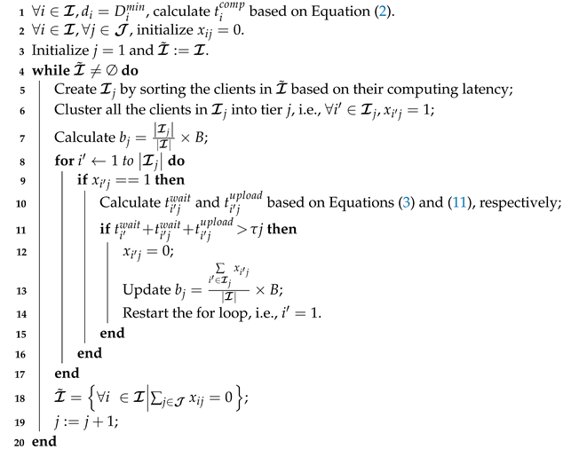
Solving remains challenging due to the unknown waiting time specified in (5), which becomes known only after clients have been grouped into tiers. However, for optimizing the objective function in , it is preferable to assign clients to lower tiers that have a larger , while still meeting the tier’s deadline constraints as outlined Constraint (5). Motivated by this insight for solving , we design the heuristic LEAD algorithm (joint cLient clustEring and bAnDwidth allocation), summarized in Algorithm 1. Specifically,
- Each client’s uploading time is determined by its tier. Additionally, tier bandwidth is determined by the number of clients in the corresponding tier, i.e., . Then,
- In the iteration, we intend to assign as many clients as possible to the tier, while satisfying Constraint (5). Let denote the set of clients who have not been clustered into any tier yet, i.e., . We sort the clients in in descending order based on their computing latency. Let denote the set of these sorted clients, i.e., , where is the index of the clients in . Assume that all the clients in can be assigned in tier j, i.e., . We then iteratively check the feasibility of all the clients in tier j starting from the first client, i.e., whether each client in tier j can really be assigned to tier j to meet Constraint (5) or not. If a client currently in tier j cannot meet Constraint (5), this client will be removed from tier j, i.e., . Note that removing a client reduces the bandwidth allocated to tier j in Step 13, which may lead to the clients, who were previously feasible to be assigned to tier j to meet Constraint (5), no longer feasible because of the decreasing of . As a result, we have to go back and check the feasibility of all the clients in tier j starting from the first client again, i.e., in Step 14.
- Once the client clustering in tier j is finished, we start to assign clients to tier by following the same procedure in Steps 5–19. The client clustering ends when all clients have been assigned to the existing tiers, i.e., .
| Algorithm 1: LEAD algorithm |
 |
4.2. Dynamic Workload Optimization
Plugging client clustering and bandwidth allocation , which are derived by the LEAD algorithm, into , we have
Assume that , is a continuous variable. Then, is a linear programming problem, and its optimal solution can be derived by using the Simplex method in polynomial time [38]. Note that the number of samples should be an integer variable, and so we simply take to be the maximum integer value that is smaller than , i.e., , , where is the optimal value by using the Simplex method to solve .
4.3. Summary of DecantFed
The DecantFed algorithm is summarized in Algorithm 2. Specifically, the FL server performs the following steps: (1) Obtains the states in terms of channel gain , CPU frequency , and transmission power of all the clients; (2) Calculates the bandwidth allocation and client clustering based on LEAD in Algorithm 1 as well as the workload by using Simplex method to solve ; (3) Broadcasts the workload assignment , bandwidth allocation , client clustering , deadline , and the initial global model to all the clients such that all the clients can understand their local training configurations; (4) Conducts FL training for a number of global iterations. Here, in the global iteration, the FL server only collects models from the clients whose tiers are participating in training during the global iteration. That is, if , then tier j is participating in training during the global iteration. Let denote the set of the clients that are participating in the training during the global iteration, i.e., . Once the FL server receives the local models from all the clients in , it then updates the global model based on
where is the local model uploaded from client i in the global iteration, is the global model derived in the global iteration, is the local dataset of client i, and is the total number of samples in . Once the FL server has updated the global model based on (13), it broadcasts to the clients in and then initializes the next global iteration.
| Algorithm 2: DecantFed algorithm |
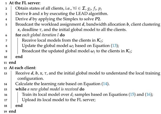 |
In DecantFed, each client trains the received global model based on its number of local samples. However, the local training may have the following: (1) The model staleness problem due to the semi-synchronous nature; (2) The model divergence problem due to the non-IID and workload optimization. Here, we apply the following solutions to tackle the model staleness and divergence problems.
- Dynamic learning rate. Similar to asynchronous FL, the model staleness problem may also exist in DecantFed, although it is mitigated. The reason for having staleness in DecantFed is that clients in high tiers may train their local models based on outdated global models. To further mitigate the model staleness problem in DecantFed, we adopt the method in [31] to set up different learning rates for the clients in different tiers, i.e.,where is the learning rate of the clients in tier j, is the learning rate of the clients in tier 1, and () is a hyperparameter to adjust the changes in learning rates among tiers. Note that both and are given before the FL training starts. Basically, Equation (14) indicates that clients in a higher tier would have a larger learning rate (i.e., ) to update their local models more aggressively such that these clients can catch up with the model update speed of the clients in the lower tiers. Note that Equation (14) also ensures that is less than 0.1 to avoid the clients in higher tiers overshooting the optimal model that minimizes the loss function. Once the learning rate is determined, client i updates its local model based on the gradient descent method, i.e.,where is the local model of client j during the t and local iterations, respectively, in the global iteration, is the input-output pair for client i’s data sample, implies the learning rate of client i, and is the loss function of the model given the model parameter and data sample . A typical loss function that has been widely applied in image classification is cross-entropy loss.
- Clipping the loss function values. Owing to the non-IID and dynamic workload optimization, the data samples in a client could be highly uneven. For example, a client has one thousand images labeled as dogs but only two images labeled as cats. If this client has high computing capability and the FL server would assign a high workload in terms of training a machine-learning model to classify dogs and cats by selecting all the images for many epochs, then the local model may overfit the client’s local dataset. After being trained by numerous dog images, the local model may diverge if a cat image is fed into the local model to generate an excessive loss value. For example, if the loss function is defined as the cross-entropy loss, then the loss function is , where is the probability of labeling the image as a cat by the local model. Infinite loss values lead to large backpropagation gradients, which can subsequently turn both weights and biases into ‘NaN’. Although regularization methods can reduce the variance of model updates, especially in IID scenarios, they cannot resolve the infinite loss issues that normally happen when the data distribution is highly non-IID. In such cases, loss clipping serves as an effective and computationally efficient solution to constrain model update, clipping the loss value into a reasonable range, i.e.,where is a hyperparameter that defines the maximum loss function value.
5. Simulations
5.1. Simulation Setup
Assume that there are 100 clients that are randomly distributed over a 2 km 2 km area to participate in the FL training via a wireless network, where a BS is located at the center of the area to forward global/local models between the FL server and clients. In addition, the path loss between a client and the BS is estimated based on [39], where and are the path loss and distance between the BS and client i. If fast fading is not considered, the channel gain between the BS and client i is mainly determined by the path loss, i.e., . Moreover, the transmission power of each client is watt, i.e., . The amount of bandwidth available for the BS is MHz. Also, the CPU frequency of a client and the number of CPU cycles to process a single sample are randomly selected, following based on two uniform distributions, i.e., Hz and CPU cycles. Other simulation parameters are listed in Table 1.

Table 1.
Simulation parameters.
5.1.1. Non-IID Dataset
Two benchmark datasets, i.e., CIFAR-10 [40] and MNIST [41], are used to evaluate the performance of DecantFed. Here, CIFAR-10 is a dataset for image classification with 10 image labels and 6000 images per label. It has 50,000 training images and 10,000 test images. MNIST is a dataset of 28 × 28 grayscale images of handwritten digits 0–9 with 60,000 training examples and 10,000 test examples.
The benchmark dataset will be dispatched to 100 clients based on non-IID across different categories, and the Dirichlet distribution is a common choice for generating non-IID data. The probability density function of the Dirichlet distribution is [42]
where is the total number of clients in the network, is the probability of dispatching an image in a dataset to client i, where , and is a parameter to adjust the degree of non-IID, i.e., a smaller leads to a more non-IID data distribution among the clients. in Equation (17) is the Gamma function, i.e., is Gamma function.
5.1.2. Global Model Design
We will train two different convolutional neural networks (CNNs) for the two benchmark datasets. For CIFAR-10, we apply a 3 VGG-block CNN with 32, 64, and 128 filters in the convolution layers. Followed by convolution layers, two fully connected layers with 128 and 10 nodes, respectively, are added, and ReLU is used as the activation function for all these layers. For MNIST, we apply a neural network having two fully connected layers with 784 and 10 nodes, respectively. The learning rates of the clients are calculated based on Equation (14), where and . The loss function value is clipped to .
5.1.3. Comparison Methods
Some FL algorithms assume that the FL server understands some prior knowledge, such as the number of samples residing on each client or the distribution of samples in each client, and design corresponding client selection or model aggregation methods to improve the model accuracy or accelerate the training process. However, we argue that this prior knowledge may not be available or accurate and violates data privacy, which is one of the major motivations for applying FL. The proposed DecantFed does not require such prior knowledge, and in order to achieve fair comparisons, two FL baselines, i.e., FedAvg [3] and FedProx [20], that also do not require such prior knowledge are used to compare the performance with DecantFed. Here, FedAvg selects all the clients in each global iteration without setting up a deadline. Also, FedAvg performs uniform local model training, meaning that the number of data samples to train a local model is the same for all the clients. On the other hand, FedProx performs synchronous FL by setting up a deadline and selects only a few clients who can upload their local models before the deadline to participate in the model training. Also, FedProx will dynamically allocate workloads to different clients based on their computing capacities. Three FL algorithms are summarized in Table 2. To compare the performance of different FL algorithms, an evaluation will be conducted on their convergence rate and model test accuracy. Since the duration of a global iteration may vary for the three FL algorithms, the convergence rates will be measured over both time and global iterations.
Table 2.
Comparisons of different FL algorithms.
5.2. Simulation Results
5.2.1. Performance Comparison Among Different FL Algorithms
Assume a deadline of s. Figure 2 shows the learning curves for different algorithms by using MNIST. Here, Figure 2a,b show the learning curves over global iterations and time, respectively, when the data distribution is more similar to non-IID (i.e., ). Similarly, Figure 2c,d show the learning curves over global iterations and time, respectively, when the data distribution is more similar to IID (i.e., ). From Figure 2a,c, we can see that, in both IID () and non-IID () scenarios, the final model accuracy of DecantFed is slightly higher than FedAvg (which is around ) but much higher than FedProx, and the convergence rate over global iteration for DecantFed is slightly faster than FedAvg. The reason for having low testing accuracy for FedProx is that FedProx only selects five clients out of one hundred, and low client participation leads to an insufficient and biased training dataset, which reduces the testing accuracy of the global model. The low client participation in FedProx also results in model accuracy decreasing when the data distribution changes from IID to non-IID. Yet, the change in model accuracy over for DecantFed and FedAvg is negligible because they allow all the clients to participate in the training. In Figure 2b,d, it is easy to observe that the convergence rate over time for DecantFed is much faster than FedAvg in both IID and non-IID scenarios. DecantFed is fully converged around s achieving model accuracy, while FedAvg only achieves and model accuracy in IID and non-IID scenarios, respectively, at s. This is because the duration of a global iteration for FedAvg is much longer than DecantFed since FedAvg has to wait for all the clients to upload the local models.
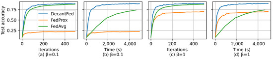
Figure 2.
Test accuracy of different algorithms for MNIST with and 1.
Figure 3 shows the learning curves for different algorithms by using CIFAR-10. We can obtain a similar conclusion in which DecantFed and FedAvg converge to a similar model test accuracy, i.e., for non-IID as shown in Figure 3a and for IID as shown in Figure 3c. On the other hand, FedProx only achieves and in non-IID and IID, respectively. This highlights that DecantFed can achieve at least higher model accuracy than FedProx. Also, the convergence rate over time for DecantFed is much faster than FedAvg in both IID and non-IID scenarios, as shown in Figure 3b,d. In order to attain a test accuracy of , DecantFed and FedAvg demand seconds and s, respectively. DecantFed is four times faster than FedAvg. It is worth noting that when as shown in Figure 3a, the final model accuracy of FedAvg is slightly better than DecantFed, which is different from the other settings. Also, the model accuracy of FedAvg during the training is more stable than DecantFed.
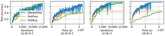
Figure 3.
Test accuracy of different algorithms for CIFAR-10 with and 1.
5.2.2. Performance of DecantFed by Varying
The deadline plays a critical role in determining the performance of DecantFed. A smaller value of enables more tiers in the system, resulting in fewer clients assigned to a tier. Hence, a smaller makes DecantFed behave more like asynchronous FL, eventually becoming asynchronous when each tier only has one client. Conversely, a larger results in DecantFed behaving more like FedAvg, i.e., all the clients are assigned to a tier, and the FL server has to wait for the last client to upload its local model if . Figure 4 shows the learning curve for different deadline settings by using CIFAR-10 when and . As shown in Figure 4a,c, a larger not only accelerates convergence over iterations but also stabilizes the training process. This is because a larger allows for more low-index-tier clients to contribute to each global update. Additionally, a larger helps global model stability. For example, there are several noticeable sudden drops in test accuracy when , which is owing to the fact that there is only an average of 1 client in the first tier, likely providing a biased local model update. Conversely, when , the training curve is more stable due to the fact that more clients are in the lower tiers. However, a larger leads to slower convergence over time owing to the longer duration of a global iteration. Table 3 shows final model accuracy (i.e., when the model is converged) by applying different values of when . Note that DecantFed with s mirrors asynchronous FL with dynamic workload optimization, where each tier has only one client, and the FL server updates the global model immediately upon receiving a local model from any client. From the table, we can observe that choosing the appropriate deadline (e.g., s) is critical to optimize the tradeoff by maximizing the final model accuracy and maximizing the convergence rate over time in DecantFed.
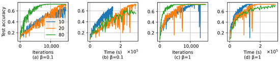
Figure 4.
Test accuracy of DecantFed with different deadlines for CIFAR-10 with and 1.
Table 3.
Test accuracy over (seconds) under non-IID with .
5.2.3. Performance of DecantFed by Optimizing the Workload Among Clients
We next evaluate how the workload optimization affects the performance of DecantFed. Here, we have two settings for DecantFed: (1) UniformDecant [42] performs uniform local training among the clients, i.e., all the clients use the same number of data samples (i.e., ) to train their local models. (2) DecantFed optimizes by solving . Other settings for UniformDecant and DecantFed are the same. Figure 5 shows the learning curves for UniformDecant and DecantFed by using CIFAR-10 when and . From the figures, we can find that DecantFed can achieve not only a higher final model accuracy but also a faster convergence rate. This basically demonstrates that dynamic workload optimization enables clients with high computational capacities to train their local models over more data samples can significantly improve the FL performance.
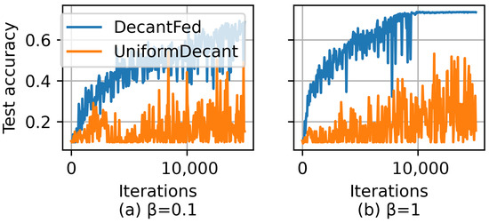
Figure 5.
Comparison of DecantFed (with dynamic workload optimization) and UniformDecant (without dynamic workload optimization) for and .
6. Conclusions
To solve the drawbacks of synchronous FL and asynchronous FL, we propose a semi-synchronous FL, i.e., DecantFed, which performs the following: (1) Jointly clusters clients into different tiers and allocates bandwidth to different tiers so that the clients in different tiers would have different deadlines/frequencies to upload their local models; (2) Dynamically allocates training workload in terms of training data samples to different clients to enable high computational capacity clients to derive better local models, while keeping the clients in their original tiers. Simulation results demonstrate that the model accuracy incurred by DecantFed and FedAvg is similar but is much higher than FedProx. The convergence rate over time incurred by DecantFed is much faster than FedAvg. In addition, the deadline is an important parameter that significantly influences the performance of DecantFed, and we will investigate how to dynamically adjust the deadline to maximize the performance of DecantFed in the future. Finally, our results demonstrate that dynamic workload optimization for clients is vital to improving FL performance. In future work, we aim to conduct an ablation study to assess the contribution of individual design components, including client clustering and bandwidth allocation, dynamic workload optimization, and dynamic learning rate, to the overall performance of DecantFed. This analysis will provide further insights into optimizing federated learning models under semi-synchronous and asynchronous settings. Such studies are expected to guide more efficient strategies tailored to heterogeneous client capabilities.
Author Contributions
Conceptualization, L.Y. and X.S.; Methodology, L.Y. and X.S.; Software, L.Y.; Validation, L.Y.; Formal analysis, L.Y.; Investigation, L.Y.; Resources, L.Y.; Data curation, L.Y.; Writing—original draft, L.Y.; Writing—review & editing, L.Y., X.S., R.A., C.P. and S.S.; Visualization, L.Y.; Supervision, X.S.; Project administration, X.S.; Funding acquisition, X.S. All authors have read and agreed to the published version of the manuscript.
Funding
This work was supported by the National Science Foundation under Award under grant no. CNS-2323050, OIA-2417062, and CNS-2148178, where CNS-2148178 is supported in part by funds from federal agencies and industry partners as specified in the Resilient & Intelligent NextG Systems (RINGS) program.
Data Availability Statement
The data presented in this study are openly available in https://arxiv.org/abs/2403.06900 (accessed on 20 November 2024).
Conflicts of Interest
The authors declare no conflicts of interest. The funders had no role in the design of the study; in the collection, analyses, or interpretation of data; in the writing of the manuscript; or in the decision to publish the results.
References
- Ansari, N.; Sun, X. Mobile Edge Computing Empowers Internet of Things. IEICE Trans. Commun. 2018, E101.B, 604–619. [Google Scholar] [CrossRef]
- Sun, X.; Ansari, N. EdgeIoT: Mobile Edge Computing for the Internet of Things. IEEE Commun. Mag. 2016, 54, 22–29. [Google Scholar] [CrossRef]
- McMahan, B.; Moore, E.; Ramage, D.; Hampson, S.; y Arcas, B.A. Communication-Efficient Learning of Deep Networks from Decentralized Data. In Proceedings of the 20th International Conference on Artificial Intelligence and Statistics, Fort Lauderdale, FL, USA, 20–22 April 2017; Volume 54, pp. 1273–1282. [Google Scholar]
- Kalloori, S.; Srivastava, A. Towards cross-silo federated learning for corporate organizations. Knowl.-Based Syst. 2024, 289, 111501. [Google Scholar] [CrossRef]
- Amini, M.R.; Feofanov, V.; Pauletto, L.; Hadjadj, L.; Devijver, E.; Maximov, Y. Self-training: A survey. arXiv 2022, arXiv:2202.12040. [Google Scholar]
- Zhang, X.; Huang, X.; Li, J. Joint Self-Training and Rebalanced Consistency Learning for Semi-Supervised Change Detection. IEEE Trans. Geosci. Remote. Sens. 2023, 61, 5406613. [Google Scholar] [CrossRef]
- Guo, J.; Liu, Z.; Chen, C.L.P. An Incremental-Self-Training-Guided Semi-Supervised Broad Learning System. IEEE Trans. Neural Netw. Learn. Syst. 2024; early access. [Google Scholar] [CrossRef]
- Sohn, K.; Berthelot, D.; Carlini, N.; Zhang, Z.; Zhang, H.; Raffel, C.A.; Cubuk, E.D.; Kurakin, A.; Li, C.L. Fixmatch: Simplifying semi-supervised learning with consistency and confidence. Adv. Neural Inf. Process. Syst. 2020, 33, 596–608. [Google Scholar]
- Fu, X.; Shi, S.; Wang, Y.; Lin, Y.; Gui, G.; Dobre, O.A.; Mao, S. Semi-Supervised Specific Emitter Identification via Dual Consistency Regularization. IEEE Internet Things J. 2023, 10, 19257–19269. [Google Scholar] [CrossRef]
- Wu, Z.; He, T.; Xia, X.; Yu, J.; Shen, X.; Liu, T. Conditional Consistency Regularization for Semi-Supervised Multi-Label Image Classification. IEEE Trans. Multimed. 2024, 26, 4206–4216. [Google Scholar] [CrossRef]
- Vu, T.T.; Ngo, D.T.; Ngo, H.Q.; Dao, M.N.; Tran, N.H.; Middleton, R.H. Straggler Effect Mitigation for Federated Learning in Cell-Free Massive MIMO. In Proceedings of the ICC 2021—IEEE International Conference on Communications, Montreal, QC, Canada, 14–23 June 2021; pp. 1–6. [Google Scholar] [CrossRef]
- Albelaihi, R.; Sun, X.; Craft, W.D.; Yu, L.; Wang, C. Adaptive Participant Selection in Heterogeneous Federated Learning. In Proceedings of the 2021 IEEE Global Communications Conference (GLOBECOM), Madrid, Spain, 7–11 December 2021; pp. 1–6. [Google Scholar] [CrossRef]
- Wang, J.; Joshi, G. Cooperative SGD: A unified framework for the design and analysis of communication-efficient SGD algorithms. arXiv 2018, arXiv:1808.07576. [Google Scholar]
- Nishio, T.; Yonetani, R. Client Selection for Federated Learning with Heterogeneous Resources in Mobile Edge. In Proceedings of the ICC 2019–2019 IEEE International Conference on Communications (ICC), Shanghai, China, 20–24 May 2019; pp. 1–7. [Google Scholar] [CrossRef]
- Xu, C.; Qu, Y.; Xiang, Y.; Gao, L. Asynchronous federated learning on heterogeneous devices: A survey. arXiv 2021, arXiv:2109.04269. [Google Scholar]
- Damaskinos, G.; Guerraoui, R.; Kermarrec, A.M.; Nitu, V.; Patra, R.; Taiani, F. FLeet: Online Federated Learning via Staleness Awareness and Performance Prediction. In Proceedings of the 21st International Middleware Conference, New York, NY, USA, 7–11 December 2020; pp. 163–177. [Google Scholar] [CrossRef]
- Rodio, A.; Neglia, G. FedStale: Leveraging stale client updates in federated learning. arXiv 2024, arXiv:2405.04171. [Google Scholar]
- Gao, Z.; Duan, Y.; Yang, Y.; Rui, L.; Zhao, C. FedSeC: A Robust Differential Private Federated Learning Framework in Heterogeneous Networks. In Proceedings of the 2022 IEEE Wireless Communications and Networking Conference (WCNC), Austin, TX, USA, 10–13 April 2022; pp. 1868–1873. [Google Scholar] [CrossRef]
- Albaseer, A.; Abdallah, M.; Al-Fuqaha, A.; Erbad, A. Data-Driven Participant Selection and Bandwidth Allocation for Heterogeneous Federated Edge Learning. IEEE Trans. Syst. Man, Cybern. Syst. 2023, 53, 5848–5860. [Google Scholar] [CrossRef]
- Li, T.; Sahu, A.K.; Zaheer, M.; Sanjabi, M.; Talwalkar, A.; Smith, V. Federated Optimization in Heterogeneous Networks. In Proceedings of the Machine Learning and Systems, Austin, TX, USA, 2–4 March 2020; Volume 2, pp. 429–450. [Google Scholar]
- Lee, J.; Ko, H.; Pack, S. Adaptive Deadline Determination for Mobile Device Selection in Federated Learning. IEEE Trans. Veh. Technol. 2022, 71, 3367–3371. [Google Scholar] [CrossRef]
- Bonawitz, K.; Eichner, H.; Grieskamp, W.; Huba, D.; Ingerman, A.; Ivanov, V.; Kiddon, C.; Konečný, J.; Mazzocchi, S.; McMahan, H.B.; et al. Towards Federated Learning at Scale: System Design. arXiv 2019, arXiv:1902.01046. [Google Scholar] [CrossRef]
- Albelaihi, R.; Yu, L.; Craft, W.D.; Sun, X.; Wang, C.; Gazda, R. Green Federated Learning via Energy-Aware Client Selection. In Proceedings of the GLOBECOM 2022–2022 IEEE Global Communications Conference, Rio de Janeiro, Brazil, 4–8 December 2022; pp. 13–18. [Google Scholar] [CrossRef]
- Yu, L.; Albelaihi, R.; Sun, X.; Ansari, N.; Devetsikiotis, M. Jointly Optimizing Client Selection and Resource Management in Wireless Federated Learning for Internet of Things. IEEE Internet Things J. 2021, 9, 4385–4395. [Google Scholar] [CrossRef]
- Xu, J.; Wang, H. Client Selection and Bandwidth Allocation in Wireless Federated Learning Networks: A Long-Term Perspective. IEEE Trans. Wirel. Commun. 2021, 20, 1188–1200. [Google Scholar] [CrossRef]
- Nguyen, J.; Malik, K.; Zhan, H.; Yousefpour, A.; Rabbat, M.; Malek, M.; Huba, D. Federated Learning with Buffered Asynchronous Aggregation. In Proceedings of the 25th International Conference on Artificial Intelligence and Statistics, Virtual, 28–30 March 2022; Volume 151, pp. 3581–3607. [Google Scholar]
- Wang, Z.; Zhang, Z.; Tian, Y.; Yang, Q.; Shan, H.; Wang, W.; Quek, T.Q.S. Asynchronous Federated Learning over Wireless Communication Networks. IEEE Trans. Wirel. Commun. 2022, 21, 6961–6978. [Google Scholar] [CrossRef]
- Jiang, J.; Cui, B.; Zhang, C.; Yu, L. Heterogeneity-Aware Distributed Parameter Servers. In Proceedings of the 2017 ACM International Conference on Management of Data, New York, NY, USA, 14–19 May 2017; SIGMOD ’17. pp. 463–478. [Google Scholar] [CrossRef]
- Zhang, W.; Gupta, S.; Lian, X.; Liu, J. Staleness-Aware Async-SGD for Distributed Deep Learning. In Proceedings of the Twenty-Fifth International Joint Conference on Artificial Intelligence, New York, NY, USA, 9–15 July 2016; AAAI Press: Washington, DC, USA, 2016. IJCAI’16. pp. 2350–2356. [Google Scholar]
- Xie, C.; Koyejo, S.; Gupta, I. Asynchronous federated optimization. arXiv 2019, arXiv:1903.03934. [Google Scholar]
- Chen, Y.; Ning, Y.; Slawski, M.; Rangwala, H. Asynchronous Online Federated Learning for Edge Devices with Non-IID Data. In Proceedings of the 2020 IEEE International Conference on Big Data (Big Data), Atlanta, GA, USA, 10–13 December 2020; pp. 15–24. [Google Scholar] [CrossRef]
- Briggs, C.; Fan, Z.; Andras, P. Federated learning with hierarchical clustering of local updates to improve training on non-IID data. In Proceedings of the 2020 International Joint Conference on Neural Networks (IJCNN), Glasgow, UK, 19–24 July 2020; pp. 1–9. [Google Scholar] [CrossRef]
- Kim, Y.; Hakim, E.A.; Haraldson, J.; Eriksson, H.; da Silva, J.M.B.; Fischione, C. Dynamic Clustering in Federated Learning. In Proceedings of the ICC 2021—IEEE International Conference on Communications, Montreal, QC, Canada, 14–23 June 2021; pp. 1–6. [Google Scholar] [CrossRef]
- Yang, Z.; Chen, M.; Saad, W.; Hong, C.S.; Shikh-Bahaei, M.; Poor, H.V.; Cui, S. Delay Minimization for Federated Learning over Wireless Communication Networks. arXiv 2020, arXiv:2007.03462. [Google Scholar] [CrossRef]
- Xu, D. Latency Minimization for TDMA-Based Wireless Federated Learning Networks. IEEE Trans. Veh. Technol. 2024, 73, 13974–13979. [Google Scholar] [CrossRef]
- Hu, Y.; Huang, H.; Yu, N. Device Scheduling for Energy-Efficient Federated Learning over Wireless Network Based on TDMA Mode. In Proceedings of the 2020 International Conference on Wireless Communications and Signal Processing (WCSP), Nanjing, China, 21–23 October 2020; pp. 286–291. [Google Scholar] [CrossRef]
- Tran, N.H.; Bao, W.; Zomaya, A.; Nguyen, M.N.H.; Hong, C.S. Federated Learning over Wireless Networks: Optimization Model Design and Analysis. In Proceedings of the IEEE INFOCOM 2019—IEEE Conference on Computer Communications, Paris, France, 29 April–2 May 2019; pp. 1387–1395. [Google Scholar] [CrossRef]
- Dantzig, G.B.; Thapa, M.N. Linear Programming; Springer: Berlin/Heidelberg, Germany, 2010. [Google Scholar]
- ETSI. Radio Frequency (RF) Requirements for LTE Pico Node B (3GPP TR 36.931 Version 9.0.0 Release 9); Technical Report ETSI TR 136 931 V9.0.0; European Telecommunications Standards Institute: Sophia Antipolis, France, 2011. [Google Scholar]
- Krizhevsky, A.; Hinton, G. Learning Multiple Layers of Features from Tiny Images. 2009. Available online: https://bibbase.org/network/publication/krizhevsky-hinton-learningmultiplelayersoffeaturesfromtinyimages-2009 (accessed on 20 November 2024).
- LeCun, Y.; Bottou, L.; Bengio, Y.; Haffner, P. Gradient-based learning applied to document recognition. Proc. IEEE 1998, 86, 2278–2324. [Google Scholar] [CrossRef]
- Yu, L.; Sun, X.; Albelaihi, R.; Yi, C. Latency-Aware Semi-Synchronous Client Selection and Model Aggregation for Wireless Federated Learning. Future Internet 2023, 15, 352. [Google Scholar] [CrossRef]
Disclaimer/Publisher’s Note: The statements, opinions and data contained in all publications are solely those of the individual author(s) and contributor(s) and not of MDPI and/or the editor(s). MDPI and/or the editor(s) disclaim responsibility for any injury to people or property resulting from any ideas, methods, instructions or products referred to in the content. |
© 2024 by the authors. Licensee MDPI, Basel, Switzerland. This article is an open access article distributed under the terms and conditions of the Creative Commons Attribution (CC BY) license (https://creativecommons.org/licenses/by/4.0/).