Article

Wind Turbine Operation Status Monitoring and Fault Prediction Methods Based on Sensing Data and Big Bang–Big Crunch Algorithm

1
Digital Grid Research Institute, China Southern Power Grid, Guangzhou 510663, China
2
School of Electrical Engineering and Automation, Wuhan University, Wuhan 430072, China
3
Institute of Next Generation Power Systems and International Standards, Wuhan University, Wuhan 430072, China
*
Authors to whom correspondence should be addressed.
Electronics 2024, 13(22), 4404; https://doi.org/10.3390/electronics13224404
Submission received: 21 June 2024 / Revised: 16 October 2024 / Accepted: 16 October 2024 / Published: 11 November 2024

Abstract

:
As wind power generation technology rapidly advances, the threat of wind turbine failures to the secure and stable operation of the power grid is gaining increasing attention. Real-time monitoring of operation status and predicting potential failures in wind turbines are indispensable requirements for the safe integration of wind power. In this paper, a model based on the least squares support vector machine (LSSVM), whose parameters are optimized by the Big Bang–Big Crunch algorithm, is constructed to improve the monitoring of wind turbine operation status and fault prediction accuracy. The research methodology consists of several key stages. Firstly, the initial wind turbine sensing data are preprocessed, utilizing factor analysis to reduce dimensionality and obtain the main influencing factors of wind turbine operation. Then, an improved failure prediction model for wind turbines, based on the least squares support vector machine, is developed using the preprocessed data. The model parameters are optimized by utilizing the Big Bang–Big Crunch optimization algorithm to enhance the prediction accuracy of wind turbine failures. Finally, the feasibility and accuracy of the proposed method are validated through a case study conducted on a regional power grid with wind farm integration.

1. Introduction

With the rapid development of modern science and technology, the problems of energy depletion and environmental pollution caused by the extensive use of fossil fuels are receiving increasing attention [1,2]. In response to these pressing challenges, countries worldwide have started to prioritize the development and utilization of renewable energy sources [3]. Clean and low-carbon energy sources like wind and solar power have gained widespread adoption [4]. Currently, wind energy accounts for a large proportion of total renewable energy and has seen sustained and rapid growth. This growth can be attributed to its advantages, such as a short construction period, environmental friendliness, and abundant wind resources [5,6]. In the future, wind power will assume a pivotal role in the shift towards a low-carbon energy mix. However, it also presents notable challenges in the realm of power system operation and maintenance. Statistically, it is common for the maintenance and repair costs of wind turbines to exceed their initial procurement expenses [7]. In the case of offshore wind turbines, maintenance costs alone account for at least 10% of the total power generation costs [8].
Renewable energy integrated into the power grid through power electronic equipment results in a significant inertia reduction and state fluctuations, fundamentally altering the conventional characteristics of the power grid [9,10,11]. In the face of equivalent disturbances, the new-type power system is more susceptible to pronounced frequency and voltage fluctuations, thereby escalating the risk of wind turbine operation going off-grid [12]. Furthermore, the unpredictability of wind power combined with potential turbine failures can lead to extensive power outages. Consequently, the industry consensus emphasizes the importance of minimizing operating costs and maximizing financial returns by avoiding excessive maintenance and the consequent downtime due to mechanical failures [13,14,15]. Therefore, it becomes imperative to monitor and forecast the operation status of wind turbines, predict potential failures, and take preemptive measures to ensure the secure and steady operation of the power grid [16,17,18].
Condition monitoring techniques have developed rapidly. Taking water turbine status prediction methods as an example, the water turbine model is a complex nonlinear dynamical system coupled by multiple factors such as water flow, machinery, and electromagnetism. The failure of the water turbine unit is characterized by complexity, diversity, coupling, and uncertainty. In addition to the mechanical vibration factors, it is usually necessary to consider the effects of electromagnetic tension of the water turbine, hydrodynamic pressure of the tailpipe and turbine, and other overcurrent components on the vibration of the unit [19]. Water turbine vibration includes three main factors, i.e., hydraulic vibration, mechanical vibration, and electromagnetic vibration. There are two types of electromagnetic vibrations. The first is rotational frequency vibration, and the other is pole frequency vibration. The characteristic frequency of rotational frequency vibration is the rotational frequency or octave frequency of the unit. Due to the uneven air gap between the hydro generator stator and rotor, the unbalanced electromagnetic force causes the violent vibration of the turbine generator rotating part. The reasons for pole frequency vibration include the loop current of the stator parallel branch generated by the unbalanced magnetic potential, negative sequence currents caused by the reversal of the magnetic potential, the stator not being round, the seat of the machine not being well sewn, etc.
The vibration analysis stands as the most commonly employed method for assessing the condition of rotating machinery under different environmental conditions, and includes power spectral density analysis, frequency-domain amplitude spectrum analysis, and cepstrum analysis. For wind turbines, mechanical vibration signals include temperature data, such as bearing temperature, oil temperature, turbine temperature, cabinet temperature, etc. [20]. The electrical data include the current, voltage, frequency, etc. The pitch data include pitch speed, pitch angle, etc. The yaw data include yaw mode, yaw angle, cabin vibration data, and other related signal data. Ref. [21] used cepstrum analysis of vibration signals to monitor the condition of rotating machinery. Ref. [22] applied cepstrum editing of vibration signals to determine bearing fault detection. However, fault-related signals in electrical signals tend to be weak compared to vibration signals, making it difficult to identify specific fault characteristics. Ref. [23] took the impeller mass imbalance of a wind turbine as the research object, analyzed the transformation characteristics of the generator electrical signals under the fault mechanism, and performed correlation analysis by using the Hilbert transform and variational modal decomposition (CA-VMD) electrical signal feature extraction method. The fault frequency was successfully extracted, and the obtained data provided a new research direction for the study of early imbalance faults in wind turbine blades. Temperature monitoring is usually applied in the fault diagnosis process of various electronic components. Ref. [24] studied the temperature data of the generator under normal operating conditions, using a linear regression technique to eliminate the effects of ambient temperature and output power, to achieve real-time reliability monitoring of generator operating temperature.
Artificial intelligence technology has been applied to generator fault predictions and diagnosis. The most widely used AI diagnostic methods are artificial neural networks (ANNs), fault trees (FTs), expert systems (ESs), support vector machines (SVMs), etc. SVM is a pattern recognition technique based on statistical learning theory, which firstly maps the feature vectors to the high-dimensional feature space, and then searches for the optimal classification hyperplane in the high-dimensional feature space to realize pattern recognition. Support vector machines can be divided into three types of optimization algorithms, i.e., SVMs, least squares support vector machines, and intelligent algorithm-based support vector machines (IAMs). In recent years, support vector machines have been widely used in the fault prediction and diagnosis of water turbines. For example, Ref. [25] proposed a K-nearest neighbor support vector data description algorithm to realize turbine generator fault diagnosis, with the spectral characteristics of the hydroelectric unit vibration signals as a special feature characterization vector. Ref. [26] proposed an improved support vector machine algorithm based on distance confidence for the problem of sample overlapping of hydro generators, which took the amplitude components of the six frequency bands of the vibration signals as fault indication to identify three typical faults of water turbines, i.e., rotor imbalance, rotor misalignment, and dynamic and static friction. A fuzzy kernel clustering algorithm based on a differential evolutionary algorithm is proposed in [27] to realize the fault diagnosis of motor bearings by extracting time-domain features and frequency-domain features of vibration signals. Generally, the support vector machine is very suitable for dealing with small-sample fault diagnosis problems and has many advantages such as high accuracy, strong robustness, and strong generalization ability in the application of traditional turbine fault diagnosis. However, in the case of wind turbines, which possess characteristics such as uncertainty of output, geographic dispersion, and high quantity, improving status monitoring and fault prediction methods deserves further study.
In recent years, machine learning and data visualization techniques have been developed rapidly, and data mining techniques have emerged. Ref. [28] proposed a method based on a data mining algorithm for early prediction of carbon brush failure, and a method is also introduced for accurately predicting the operation status of wind turbines [8]. Some researchers have constructed a wind turbine fault prediction model using the least squares support vector mechanism [29,30], which is optimized using a particle swarm optimization algorithm and genetic algorithm. However, genetic algorithms and particle swarm optimization algorithms still have the disadvantages of poor convergence and weak robustness, greatly affecting the accuracy and speed of fault diagnosis. The Big Bang algorithm, as an intelligent optimization algorithm, has received a lot of attention due to its strong function optimization ability, simple algorithm implementation, and fewer requirements for parameter setting [31].
Each wind turbine is installed with a set of SCADA systems for the operation monitoring and control of the wind turbine, with the functions of status display, historical information query, equipment control, and fault alarm [32]. Utilizing SCADA data to monitor the operation status of wind turbines avoids additional sensors, peripheral software, and hardware devices, offering great potential to improve the operation economics and reliability of the wind turbines [33]. In practice, the SCADA system still mainly uses the collected status information to control key parts of the wind turbine generators and has not yet made good use of the wind turbine data collected during the control process for status monitoring [34]. It is necessary to expand the alarm function to realize early fault identification to improve the secure operation of wind turbines [35].
To address the research gap mentioned above, a new prediction method is proposed in this paper, based on the least squares support vector mechanism and the Big Bang algorithm, to achieve more precise operation status monitoring and fault prediction for wind turbines. First, initial wind turbine sensing data were preprocessed using factor analysis to reduce dimensionality and determine the main factors. Then, based on the preprocessed data, a wind turbine failure prediction model was developed using an improved least squares support vector machine (LSSVM) method. Next, to improve the accuracy of wind turbine failure prediction, the model parameters were innovatively optimized by using the Big Bang–Big Crunch optimization algorithm. Finally, the feasibility of the proposed method is verified by a case study conducted on the regional power grid.
The rest of the paper is organized as follows: Section 2 constructs the prediction model based on the improved least squares support vector machine and describes the solution process. Section 3 innovatively optimizes the model parameters using the Big Bang–Big Crunch optimization algorithm. Section 4 performs a case study to validate the effectiveness of the proposed method. Section 5 summarizes the whole paper.

2. Modeling and Solving

The initial wind turbine sensing data collected by SCASA were preprocessed using factor analysis to reduce dimensionality [36,37,38]. Afterward, the processed data were used to identify and determine the main factors that affect wind turbine operation states.

2.1. Data Preprocessing

The initial data obtained by the SCADA system have zero values and repetitive values, potentially leading to misclassification of turbine status and increasing the data processing burden. Thus, to obtain useful and concise data, the initial data needed to be preprocessed and the procedures were as follows:
(1)
Eliminate zeros and duplicates in the database;
(2)
Fill in the missing values using the values from the previous timestamp;
(3)
Remove all data with power less than 1200 kW at wind speeds greater than 13 m/s.

2.1.1. Standardization

The factor analysis method is used to reduce data dimensionality. It is assumed that there are p indicator variables and n evaluation objects for factor analysis. The value of the j indicator for the i evaluation object is xij. By calculating the mean and standard deviation of the individual evaluation indicators for each variable, the values of the indicators xij are converted into standardized indicators x ˜ i j as follows:
x ˜ i j = x i j x ¯ J s j , ( i = 1 , 2 , , n ; j = 1 , 2 , , p )
x ¯ J = 1 n i = 1 n x i j
s j = 1 n 1 i = 1 n ( x i j x ¯ J ) 2
where x ¯ J and sj are the mean and standard deviation of the ith indicator, p is the total number of indicator variables, and n is the total number of evaluation objects.

2.1.2. Correlation Coefficient Matrix and Factor Loading Matrix

The Pearson correlation coefficient matrix of indicators was calculated as follows [39]:
R = ( r i j ) p × p
r i j = k = 1 n x ˜ k i x ˜ k j n 1
where rii = 1, rij = rji, and rij is the correlation coefficient between the ith indicator and the jth indicator.
According to the correlation coefficient matrix obtained, the eigenvalues (λ1 > λ2 > λ1... > λp > 0) and the corresponding eigenvectors (u1, u2, u1..., up) of R were calculated. The factor loading matrix A was obtained as follows:
A = [ λ 1 u 1 , λ 2 u 2 λ p u p ]
where uj = (u1j, u2j, u1..., urj).

2.1.3. Factor Rotation

Based on the factor loading matrix A, the contribution of each common factor was calculated and m primary factors were determined. The matrix B = A ^ T was obtained by rotating the extracted factor load matrix, and the factor model was constructed as follows:
x ˜ 1 = b 11 F 1 + + b 1 m F m x ˜ p = b p 1 F 1 + + b p m F m
where m is the number of primary factors (m < p), A ^ is the first m column of A, and T is an orthogonal matrix. Fi is the factor score.

2.1.4. Calculating Factor Scores and Reducing the Dimensionality

Regression methods are used to obtain the individual factor score, as shown in (8) and (9). The composite scores for each sample were then calculated to determine the main factors influencing the data, which were further used for the wind turbine failure analysis. By using the factor analysis method, the dimensionality of the initial sensing data were reduced.
F ^ j = b j 1 x ˜ 1 + + b j p x ˜ p , j = 1 , 2 , , m
b 11 b 12 b 1 p b 21 b 22 b 2 p b m 1 b m 2 b m p = b 1 b 2 b m = R 1 A

2.2. Improved LSSVM Model

An improved fault prediction model based on least squares support vector machine is constructed according to the preprocessed data [40,41,42]. To map the input space to the feature space, a nonlinear function is proposed as follows:
f ( x ) = b + ϕ ( x k ) , w
where x k = ( x k 1 , x k 2 , , x k m ) is the input vector of m dimension, w is the weight vector, b is the bias term, and the symbol refers to the inner product operation. ϕ ( x k ) is a nonlinear function that maps the input space to the feature space.
The evaluation problem is described as an optimization problem with the structured risk minimization as the objective function:
min w , b , e J ( w , e ) = 1 2 w T w + 1 2 γ k = 1 N e k 2 s . t . y k [ w T ϕ ( x k ) + b ] = 1 e k k = 1 , 2 , , N
where yk is the output variable, ek is the slack variable, γ is the penalty factor, and N is the total number of training samples.

2.2.1. Application of the Lagrange Multiplier Method

The model developed is an optimization model with equation constraints, which is difficult to solve directly. The corresponding Lagrangian function is constructed to transform the original problem into an optimization problem without equation constraints [43,44].
L ( w , b , e , α ) = J ( w , e ) k = 1 N α k w T ϕ ( x k ) b + e k y k
J ( w , e ) = 1 2 w 2 + 1 2 γ k = 1 N e k 2                         s . t . γ > 0
where ak is the Lagrange multiplier.
According to the optimization theory, the optimal solution of an optimization problem without constraints should satisfy the condition that the partial derivatives of the objective function with respect to each variable are zero [45,46], as shown in (14). Via substituting (12) and (13) into (14) and performing derivatives for variables (i.e., w, b, ek, ak), the optimal solution condition can be obtained as (15).
L w = 0 L b = 0 L e k = 0 L α k = 0
w = k = 1 N α k ϕ ( x k ) k = 1 N α k = 0 α k = γ e k w T φ ( x k ) + b + e k y k = 0
where L is the Lagrange function.

2.2.2. Equation Transformation

From (15), the variables w and ek can be expressed as functions of variable ak. By replacing w and ek with functions of variable ak, Equation (16) can be obtained for ease of solution. Via further analysis and deformation, (16) is finally expressed as a matrix form in (17) and (18). K(xk, xl) is the kernel function, which can reduce the computational complexity of high-dimensional spaces. The kernel function plays an important role in constructing high-performance least squares support vector machines.
k = 1 N α k = 0 k = 1 N α k φ ( x k ) T φ ( x k ) + b + α k γ y k = 0
0 1 v T 1 v Ω + I / γ b α = 0 y
α = α 1 α k α N T Ω = φ ( x k ) T φ ( x l ) = K ( x k , x l )
where α is the Lagrange multiplier vector, and Ω is the kernel function.

2.2.3. LSSVM Regression Function

Through the above process, the LSSVM model can be represented as (19) by using LSSVM regression function.
y ( x ) = k = 1 N α k K ( x , x k ) + b
The radial basis function (RBF) kernel is adopted for analysis in this paper as follows:
K ( x k , x l ) = exp x k x l 2 2 σ 2 , σ > 0
where σ is the bandwidth of the kernel function, which is a significant factor in the performance of the LSSVM model.

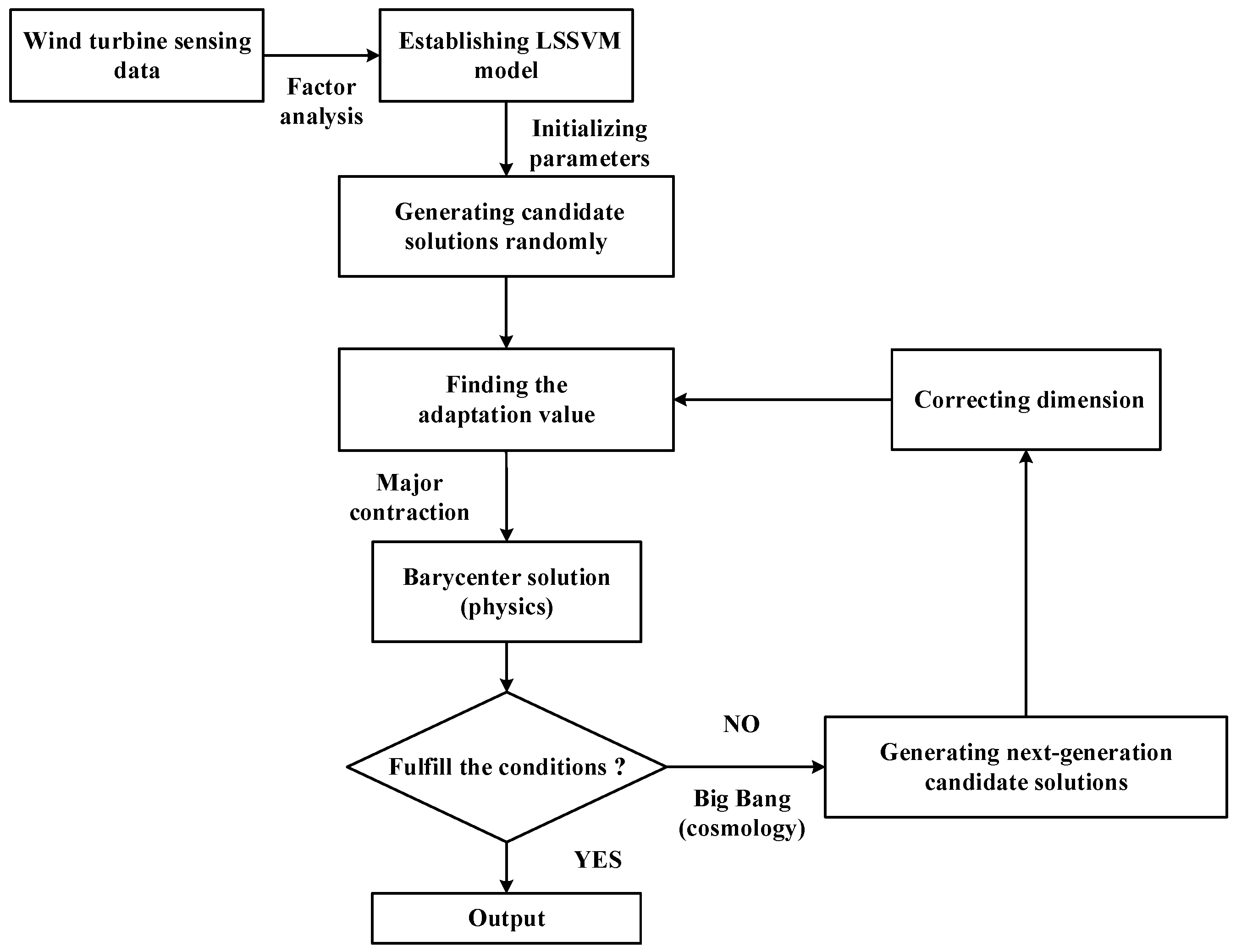
3. Parameter Optimization for LSSVM Model Based on the Big Bang–Big Crunch Algorithm

The Big Bang–Big Crunch algorithm is proposed to optimize the improved wind turbine failure prediction model based on the LSSVM [47,48,49]. The procedures of the Big Bang–Big Crunch algorithm used to optimize the model parameters are illustrated in Figure 1.

3.1. Model Parameter Optimization

It is assumed that the initial value of the iteration number t is set to 0, and the maximum number of iterations is set to T. Treating the parameters of the LSSVM model as a population, the solution set of the Big Bang–Big Crunch algorithm is initialized in the problem solution search space.

3.1.1. Contraction Process

The fitness value of each fragment solution is calculated using the fitness function, and the contemporary mass center is obtained by the singularity contraction formula, as shown in (21).
X c k = i = 1 M 1 f i X i k i = 1 M 1 f i
where Xck denotes the kth coordinate component of the contemporary shrinkage mass center in the nth dimension space, fi is the fitness value of the ith fragment solution, and M is the total number of contemporary fragmentation solutions.

3.1.2. Big Bang Process

Based on the contemporary mass center, the next generation of fragment solutions is obtained through the Big Bang process, as shown in (22). Meanwhile, the optimal solutions are retained for the next generation of fragment solution sets, and solution dimension correction is performed for the obtained solution set.
X i k = X c k + r a ( x max x min ) 1 + t
where Xik denotes the kth coordinate component of the ith fragment solution; r is a random value between (−1, 1), which obeys the Gaussian distribution; a is the shrinkage factor, which is a constant during the Big Bang process; t is the number of iterations; and xmax and xmin are the upper and lower bounds of the solution space.

3.2. Decision-Making

The contraction process and Big Bang process are performed cyclically, until the stopping criterion is satisfied or the number of iterations reaches the maximum T. If the criterion is met, the obtained prediction results are sent to the expert system for further analysis to obtain the failure diagnosis results. The detailed decision-making steps to determine the reason for wind turbine failure are as follows:
(1)
The obtained prediction results are sent to the expert system information base to be saved and then sent to the reasoning machine;
(2)
The reasoning machine performs deductive analysis on the prediction results and repeatedly matches the established rules in the information base to derive the reason for the wind turbine failure;
(3)
The reason for the wind turbine failure is fed into the explanation mechanism. The corresponding explanation is drawn and presented on the human–computer interaction interface, according to the deductive analysis process and obtained results.
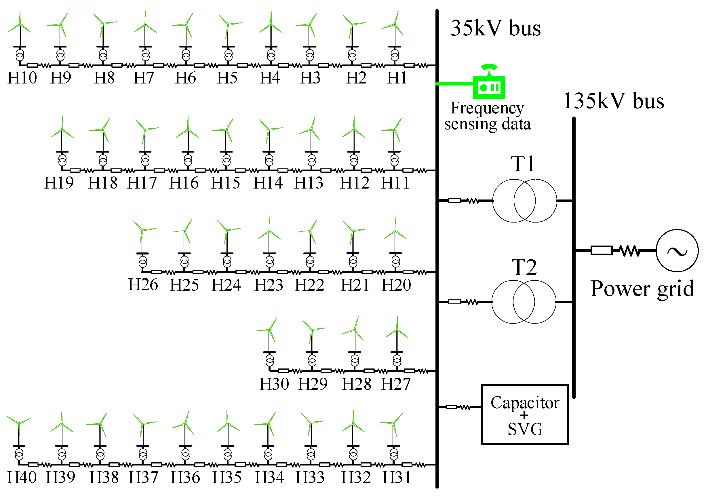
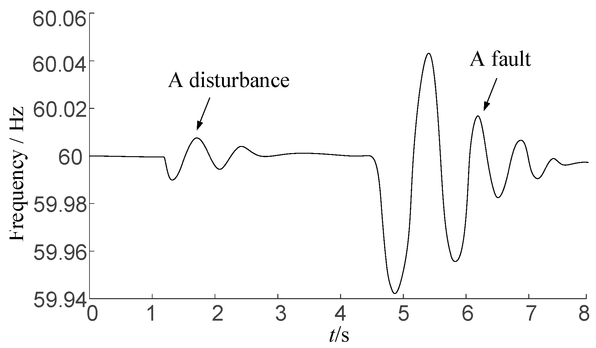
In general, utilizing factor analysis, the initial wind turbine sensing data are preprocessed to reduce dimensionality and obtain the primary factors. An improved failure prediction model for wind turbines based on the LSSVM model is established, whose parameters are optimized using the proposed Big Bang–Big Crunch optimization algorithm. By using the proposed method, the prediction accuracy of wind turbine failure is enhanced, eventually improving the safe and economic operation of wind farms.

4. Case Study

A case study was conducted on a regional power grid with a wind farm connected to illustrate the effectiveness of the proposed method, as shown in Figure 2 and Figure 3. The least squares support vector machine is used to improve the monitoring of wind turbine operation status and fault prediction accuracy, whose parameters are optimized by the Big Bang–Big Crunch algorithm. As mentioned above, the support vector machine is suitable for dealing with small-sample fault diagnosis problems with high accuracy and strong robustness. The operation data, such as temperature, current, voltage, frequency, and vibration data, can also be utilized to analyze the performance of the proposed method. In this case study, the frequency data are taken as an example to validate the feasibility of the proposed method. The SCADA data of a wind farm and the frequency at the grid-side of the grid-connected point are collected as characteristic indicators of wind turbine failure trends. By monitoring and analyzing the grid frequency and predicting its development trend, the potential failure problems of wind turbines are judged and predicted.
In general, the performance of a prediction model is quantified by metrics such as MAE, MSE, and RMSE. MAE is the mean absolute error, i.e., the absolute value of residuals, and represents the average of the absolute errors between the predicted values and the observed values, as shown in (23). MSE is the mean square error, which is obtained via the square operation, sum operation, and average operation of the interpolated value between the true value and the predicted value, as shown in (24). RMSE is the root mean square error, measuring the deviation between the predicted value and the true value, which is more sensitive to outliers in the data, as shown in (25).
M A E = 1 N i = 1 N y ^ i y i
M S E = 1 N i = 1 N ( y i y ^ i ) 2
R M S E = 1 N i = 1 N ( y i y ^ i ) 2
In the case study, 80% of the SCADA data are used for the training set to construct the LSSVM prediction model, and the rest of the data are used as a test dataset for validating the feasibility of the established model. It is assumed that a disturbance and a fault occurred at wind turbine H15 within the time period, as shown in Figure 4.
The effectiveness of the proposed wind turbine failure prediction model based on the improved LSSVM is validated by comparing it with the conventional method, in which the Big Bang–Big Crunch algorithm is not used, as shown in Table 1. A total of 1000 sample points are taken in the time window, and the mathematical properties of the predicted frequency, including the mean absolute error and mean square error, for the different methods are obtained, as shown in Figure 5, Figure 6, Figure 7, Figure 8, Figure 9 and Figure 10.
In the simulation based on the test set, the frequency response ranged from fN − 0.06 to fN + 0.06, as shown in Figure 5 and Figure 6. Generally, the predicted frequency indicator and true frequency response are linearly correlated, as represented by the dotted lines. However, compared to the conventional method, there is less dispersion and a greater correlation between true frequency response and the predicted frequency indicator for the improved LSSVM method, which intuitively proves a higher prediction accuracy of the proposed method.
The absolute error and square error are used to mathematically compare the performance of the two methods. The absolute errors of the proposed method are smaller than those of the conventional method, as shown in Figure 7 and Figure 8, which means that the prediction accuracy of the proposed model is generally higher than that of the conventional SVM when frequency fluctuations occur due to wind turbine disturbances and faults. Similarly, the square errors of the proposed method are smaller than those of the conventional method, as shown in Figure 9 and Figure 10. Using the statistics in Table 1, the MAE of the proposed method is reduced by 86.10%, the MSE of the proposed method is 1.92% of that of the conventional method, and the RMSE of the proposed method is 13.83% of that of the conventional method. Thus, the method based on the LSSVM optimized by the Big Bang–Big Crunch algorithm could effectively improve wind turbine state prediction performance.

5. Conclusions

In this paper, a prediction model for improving the operation status monitoring and fault prediction accuracy of wind turbines is constructed based on the least squares support vector machine and the Big Bang–Big Crunch optimization algorithm. Factor analysis is used for dimensionality reduction of the complicated operating data of wind turbines, to more accurately capture the main characteristic variables for detecting wind turbine failures. Aiming to combat the limitations of the conventional LSSVM, the Big Bang algorithm, with better convergence and robustness, is innovatively used to optimize the parameters of the established prediction model and enhance its failure prediction accuracy. The case study conducted on the regional power grid verifies that the proposed method based on the improved LSSVM achieves more precise prediction, improving the wind turbine failure prediction accuracy compared with the conventional method. In future work, the proposed failure prediction method based on the improved LSSVM will be further extended and applied in a multi-energy system, with wind power, solar power, thermal energy, and natural gas integration, to achieve higher-accuracy failure prediction for different types of equipment.

Author Contributions

P.L.: conceptualization, resources, writing, supervision, methodology, original draft preparation, project administration. B.T.: methodology, reviewing, editing. Z.L.: writing, methodology, investigation. Z.W.: investigation. Y.L.: investigation, validation. X.Y.: investigation. J.Z.: editing, investigation. B.L.: investigation. Z.Z.: writing, reviewing, editing. All authors have read and agreed to the published version of the manuscript.

Funding

This research was funded by the Science and Technology Project of China Southern Power Grid Company, grant number SYYKJXM20210055.

Data Availability Statement

The data that support the findings of this study are available from the corresponding author upon reasonable request.

Conflicts of Interest

Authors Peng Li, Bing Tian, Zhong Liu, Yuehuan Lin, Zhiming Wang, Xu Yin, Jiaming Zhang and Baifeng Luo were employed by the company China Southern Power Grid. The remaining authors declare that the research was conducted in the absence of any commercial or financial relationships that could be construed as a potential conflict of interest.

References

  1. Cao, X.; Liu, C.; Wu, M.; Li, Z.; Wang, Y.; Wen, Z. Heterogeneity and connection in the spatial-temporal-evolution trend of China’s energy consumption at provincial level. Appl. Energy 2023, 336, 120842. [Google Scholar] [CrossRef]
  2. Tapiero, C.S. Energy consumption and environmental pollution: A stochastic model. IMA J. Manag. Math. 2009, 20, 263–273. [Google Scholar] [CrossRef]
  3. Zhang, Z.; Lin, Y.; Fan, J.; Han, Z.; Fan, Y.; Shu, Y. Implicit-integral dynamic optimization based on spatial partitioning and temporal segmentation for the power jumps of renewable energy sources. Appl. Energy 2025, 377 Pt A, 124471. [Google Scholar] [CrossRef]
  4. Zhang, Z.; Han, Z.; Hu, H.; Fan, Y.; Fan, J.; Shu, Y. Self-adaptive system state optimization based on nonlinear affine transformation for renewable energy volatility. Renew. Energy 2024, 230, 120846. [Google Scholar] [CrossRef]
  5. Junjun, L.; Zhengqiu, W.; Xunqiong, T.; Bo, C. Review of wind power generation and relative technology development. Electr. Power Constr. 2011, 32, 64–72. [Google Scholar]
  6. Zhang, B.; Yang, Y. Status and trend of wind & photovoltaic power development. Electr. Power 2006, 39, 65–69. [Google Scholar]
  7. Walford, C. Wind Turbine Reliability: Understanding and Minimizing Wind Turbine Operation and Maintenance Costs; Rep. SAND-2006-1100; Sandia National Laboratories: Albuquerque, NM, USA, 2006. [Google Scholar]
  8. Kusiak, A.; Verma, A. A Data-Mining Approach to Monitoring Wind Turbines. IEEE Trans. Sustain. Energy 2012, 3, 150–157. [Google Scholar] [CrossRef]
  9. Arredondorodriguez, F.; Ledesma, P.; Castronuovo, E.D.; Aghahassani, M. Stability Improvement of a Transmission Grid With High Share of Renewable Energy Using TSCOPF and Inertia Emulation. IEEE Trans. Power Syst. 2020, 37, 3230–3237. [Google Scholar] [CrossRef]
  10. Zhang, Z.; Wang, Z.; Shang, B.; Fan, Y.; Shu, Y. Event-triggered reactive power tracking optimization for second-level power fluctuations of renewables and stochastic loads. Int. J. Electr. Power Energy Syst. 2024, 155, 109581. [Google Scholar] [CrossRef]
  11. Zhang, Z.; Shang, L.; Liu, C.; Lai, Q.; Jiang, Y. Consensus-based distributed optimal power flow using gradient tracking technique for short-term power fluctuations. Energy 2023, 264, 125635. [Google Scholar] [CrossRef]
  12. Ulbig, A.; Borsche, T.S.; Andersson, G. Impact of Low Rotational Inertia on Power System Stability and Operation. IFAC Proc. Vol. 2014, 47, 7290–7297. [Google Scholar] [CrossRef]
  13. Faulstich, S.; Hahn, B.; Tavner, P.J. Wind turbine downtime and its importance for offshore deployment. Wind Energy 2011, 14, 327–337. [Google Scholar] [CrossRef]
  14. Qiao, W.; Lu, D. A survey on wind turbine condition monitoring and fault diagnosis-Part I: Components and subsystems. IEEE Trans. Ind. Electron. 2015, 62, 6536–6545. [Google Scholar] [CrossRef]
  15. Amirat, Y.; Benbouzid, M.E.H.; Al-Ahmar, E.; Bensaker, B.; Turri, S. A brief status on condition monitoring and fault diagnosis in wind energy conversion systems. Renew. Sustain. Energy Rev. 2009, 13, 2629–2636. [Google Scholar] [CrossRef]
  16. Hu, X.; Tang, T.; Tan, L.; Zhang, H. Fault Detection for Point Machines: A Review, Challenges, and Perspectives. Actuators 2023, 12, 391. [Google Scholar] [CrossRef]
  17. Jing, X.; Wu, Z.; Zhang, L.; Li, Z.; Mu, D. Electrical Fault Diagnosis From Text Data: A Supervised Sentence Embedding Combined With Imbalanced Classification. IEEE Trans. Ind. Electron. 2024, 71, 3064–3073. [Google Scholar] [CrossRef]
  18. Zhu, D.; Wang, Z.; Hu, J.; Zou, X.; Kang, Y.; Guerrero, J.M. Rethinking Fault Ride-Through Control of DFIG-Based Wind Turbines from New Perspective of Rotor-Port Impedance Characteristics. IEEE Trans. Sustain. Energy 2024, 15, 2050–2062. [Google Scholar] [CrossRef]
  19. Zhu, W. Research on Methods of Fault Diagnosis, Prognostics and Condition Assessment for Hydroelectric Generator Units; Huazhong University of Science & Technology: Wuhan, China, 2017. [Google Scholar]
  20. Badihi, H.; Zhang, Y.; Jiang, B.; Pillay, P.; Rakheja, S. A Comprehensive Review on Signal-Based and Model-Based Condition Monitoring of Wind Turbines: Fault Diagnosis and Lifetime Prognosis. Proc. IEEE 2022, 110, 754–806. [Google Scholar] [CrossRef]
  21. Zheng, G.T.; Wang, W.J. A new cepstral analysis procedure of recovering excitations for transient components of vibration signals and applications to rotating machinery condition monitoring. J. Vib. Acoust. 2001, 123, 222–229. [Google Scholar] [CrossRef]
  22. Cedric, P.; Patrick, G.; Jan, H. Vibration-based bearing fault detection for operations and maintenance cost reduction in wind energy. Renew. Energy 2018, 116, 74–87. [Google Scholar]
  23. Dang, J.; Wei, J.; Li, J. Feature Extraction Method for Unbalanced Fault Electrical Signal of Wind Turbine Impeller Based on Hilbert and CA -VMD. Power Syst. Clean Energy 2021, 37, 112–118+126. [Google Scholar]
  24. Huo, J.; Tang, G.; Liu, D. A novel monitoring method of wind turbine generator real-time reliability based on temperature signals. Renew. Energy Resour. 2016, 34, 408–412. [Google Scholar]
  25. Fu, W.; Zhou, J.; Li, C.; Xiao, H.; Xiao, J.; Zhu, W. Vibrant Fault Diagnosis for Hydro-Electric Generating Unit Based on Support Vector Data Description Improved With Fuzzy K Nearest Neighbor. Proc. CSEE 2014, 34, 5788–5795. [Google Scholar]
  26. Zhang, X.; Zhou, J.; Wang, C.; Li, C. Vibrant fault diagnosis for hydroelectric generator unit considering overlapping fault patterns. Power Syst. Prot. Control 2012, 40, 8–14. [Google Scholar]
  27. Zhang, X.; Zhang, X.; Liu, J. Fuzzy kernel-clustering algorithm based on differential evolution algorithm and its application in fault diagnosis. Power Syst. Prot. Control 2014, 42, 102–106. [Google Scholar]
  28. Verma, A.; Kusiak, A. Fault Monitoring of Wind Turbine Generator Brushes: A Data-Mining Approach. J. Sol. Energy Eng. 2012, 134, 021001. [Google Scholar] [CrossRef]
  29. Kaytez, F.; Taplamacioglu, M.C.; First, H. Forecasting electricity consumption: A comparison of regression analysis, neural networks and least squares support vector machines. Electr. Power Energy Syst. 2015, 67, 431–438. [Google Scholar] [CrossRef]
  30. Jindal, A.; Dua, A.; Kaur, K.; Singh, M.; Kumar, N.; Mishra, S. Decision Tree and SVM-Based Data Analytics for Theft Detection in Smart Grid. IEEE Trans. Ind. Inform. 2016, 12, 1005–1016. [Google Scholar] [CrossRef]
  31. Wu, W.; Tian, L.; Lin, Z. Hybrid Big Bang Crunch Algorithm Based on Particle Swarm Optimization. J. Guangdong Univ. Technol. 2016, 33, 12–17. [Google Scholar]
  32. Karadayi, B.; Kuvvetli, Y.; Ural, S. Fault-related Alarm Detection of a Wind Turbine SCADA System. In Proceedings of the 2021 3rd International Congress on Human-Computer Interaction, Optimization and Robotic Applications (HORA), Ankara, Turkey, 11–13 June 2021; pp. 1–5. [Google Scholar]
  33. Liu, P.; Li, Z.; Zhuo, Y.; Lin, X.; Ding, S.; Khalid, M.S.; Adio, O.S. Design of Wind Turbine Dynamic Trip-Off Risk Alarming Mechanism for Large-Scale Wind Farms. IEEE Trans. Sustain. Energy 2017, 8, 1668–1678. [Google Scholar] [CrossRef]
  34. Liu, Y.; Wu, Z.; Wang, X. Research on Fault Diagnosis of Wind Turbine Based on SCADA Data. IEEE Access 2020, 8, 185557–185569. [Google Scholar] [CrossRef]
  35. Du, B.; Narusue, Y.; Furusawa, Y.; Nishihara, N.; Indo, K.; Morikawa, H.; Iida, M. Clustering Wind Turbines for SCADA Data-Based Fault Detection. IEEE Trans. Sustain. Energy 2023, 14, 442–452. [Google Scholar] [CrossRef]
  36. Jeong, D.; Park, C.; Ko, Y.M. Missing data imputation using mixture factor analysis for building electric load data. Appl. Energy 2021, 304, 117655. [Google Scholar] [CrossRef]
  37. Li, W.; Ji, Z.; Dong, F. Global renewable energy power generation efficiency evaluation and influencing factors analysis. Sustain. Prod. Consum. 2022, 33, 438–453. [Google Scholar] [CrossRef]
  38. Sovacool, B.K. A qualitative factor analysis of renewable energy and Sustainable Energy for All (SE4ALL) in the Asia-Pacific. Energy Policy 2013, 59, 393–403. [Google Scholar] [CrossRef]
  39. Wang, G.-J.; Xie, C.; Chen, S.; Yang, J.-J.; Yang, M.-Y. Random matrix theory analysis of cross-correlations in the US stock market: Evidence from Pearson’s correlation coefficient and detrended cross-correlation coefficient. Phys. A Stat. Mech. Its Appl. 2013, 392, 3715–3730. [Google Scholar] [CrossRef]
  40. Zhang, Y.; Wang, P.; Zhang, C.; Lei, S. Wind energy prediction with LS-SVM based on Lorenz perturbation. J. Eng. 2017, 2017, 1724–1727. [Google Scholar] [CrossRef]
  41. Liu, L.; Liu, Z.; Qian, X. Rolling bearing fault diagnosis based on generalized multiscale mean permutation entropy and GWO-LSSVM. IET Sci. Meas. Technol. 2023, 17, 243–256. [Google Scholar] [CrossRef]
  42. Chen, W.; Li, J.; Wang, Q.; Han, K. Fault feature extraction and diagnosis of rolling bearings based on wavelet thresholding denoising with CEEMDAN energy entropy and PSO-LSSVM. Measurement 2021, 172, 108901. [Google Scholar] [CrossRef]
  43. Santos, A., Jr.; da Costa, G.R.M. Optimal-power-flow solution by Newton’s method applied to an augmented Lagrangian function. IEE Proc.-Gener. Transm. Distrib. 1995, 142, 33–36. [Google Scholar] [CrossRef]
  44. Bakirtzis, A.; Zoumas, C. Lambda of Lagrangian relaxation solution to unit commitment problem. IEEE Proc.—Gener. Transm. Distrib. 2000, 147, 131–137. [Google Scholar] [CrossRef]
  45. Agarwal, D.; Singh, P.; El Sayed, M.A. The Karush–Kuhn–Tucker (KKT) optimality conditions for fuzzy-valued fractional optimization problems. Math. Comput. Simul. 2023, 205, 861–877. [Google Scholar] [CrossRef]
  46. Singh, D.; Dar, B.; Kim, D. KKT optimality conditions in interval valued multiobjective programming with generalized differentiable functions. Eur. J. Oper. Res. 2016, 254, 29–39. [Google Scholar] [CrossRef]
  47. Azizian, D.; Gharehpetian, G.B. Split-winding transformer design using new hybrid optimisation algorithm based on PSO and I-BB-BC. IET Sci. Meas. Technol. 2018, 12, 712–718. [Google Scholar] [CrossRef]
  48. Mbuli, N.; Ngaha, W. A survey of big bang big crunch optimisation in power systems. Renew. Sustain. Energy Rev. 2022, 155, 111848. [Google Scholar] [CrossRef]
  49. Prayogo, D.; Cheng, M.-Y.; Wu, Y.-W.; Herdany, A.A.; Prayogo, H. Differential Big Bang—Big Crunch algorithm for construction-engineering design optimization. Autom. Constr. 2018, 85, 290–304. [Google Scholar] [CrossRef]
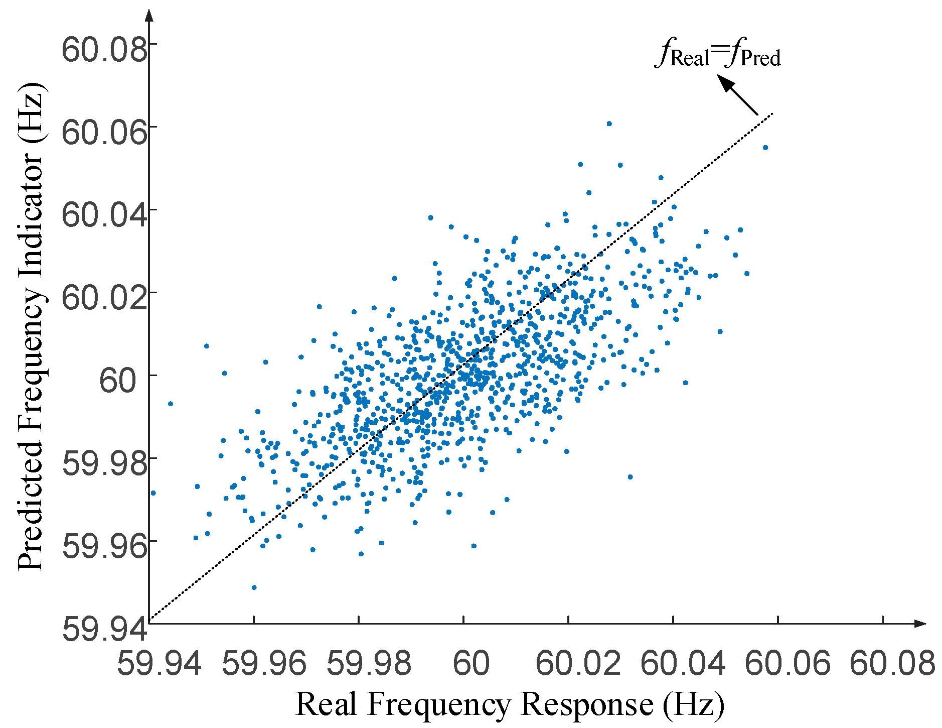
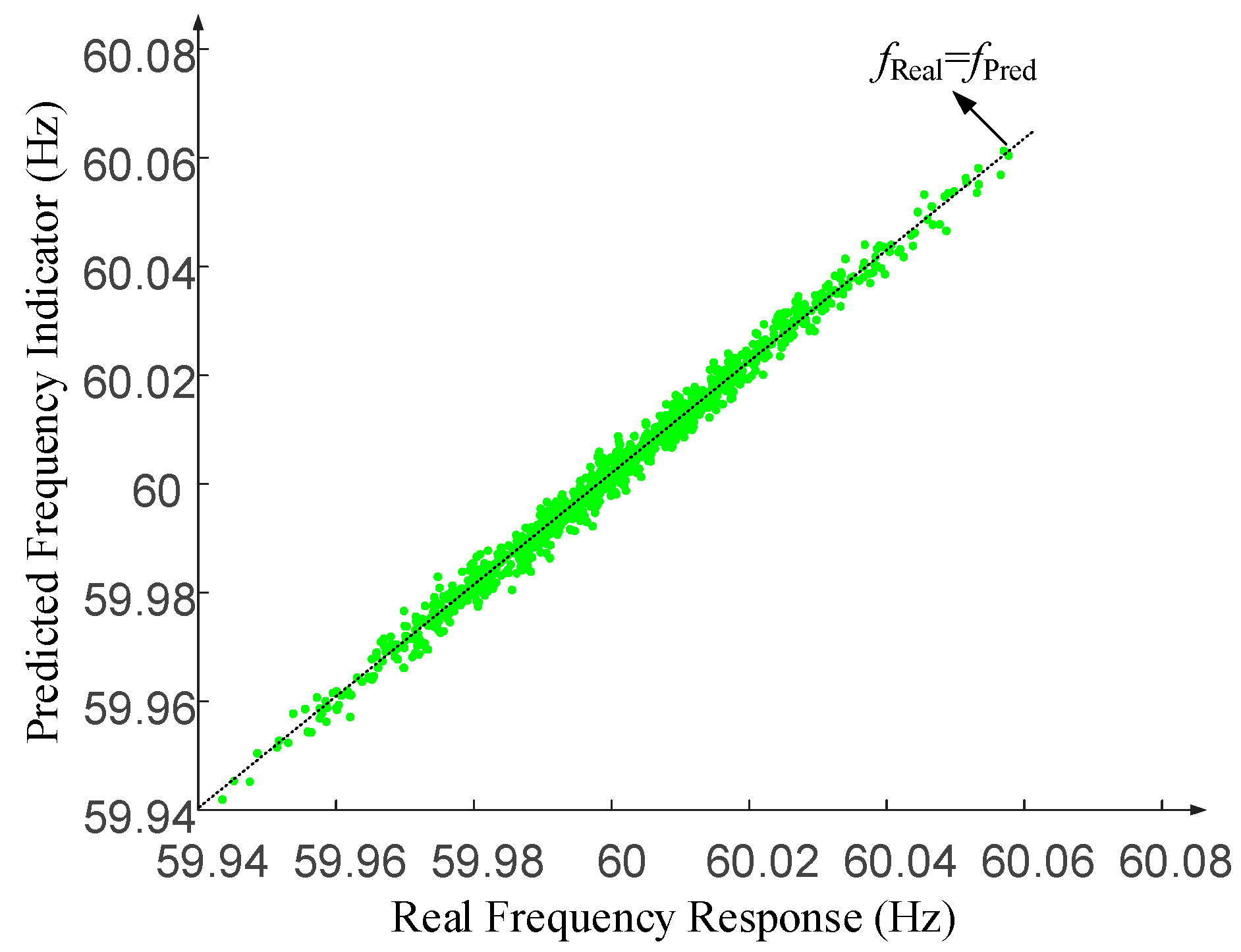
Figure 1. The solving procedures of the Big Bang–Big Crunch algorithm.
Electronics 13 04404 g001
Figure 2. Topology of the power grid with a wind firm connected.
Electronics 13 04404 g002
Figure 3. Topology of the wind farm.
Electronics 13 04404 g003
Figure 4. Frequency measured when disturbance and fault occur.
Electronics 13 04404 g004
Figure 5. Test results of the conventional SVM.
Electronics 13 04404 g005
Figure 6. Test results of the proposed LSSVM optimized by the Big Bang–Big Crunch algorithm.
Electronics 13 04404 g006
Figure 7. Absolute errors of the conventional SVM.
Electronics 13 04404 g007
Figure 8. Absolute errors of the proposed LSSVM optimized by the Big Bang–Big Crunch algorithm.
Electronics 13 04404 g008
Figure 9. Square errors of the conventional SVM.
Electronics 13 04404 g009
Figure 10. Square errors of the proposed LSSVM optimized by the Big Bang–Big Crunch algorithm.
Electronics 13 04404 g010
Table 1. Comparison of different methods.
Different MethodsConventional MethodProposed Method
AlgorithmSVMImproved LSSVM with parameters optimized by Big Bang–Big Crunch algorithm
Measured DataFrequency
MAE (Hz)1.187 × 10−21.65 × 10−3
MSE (Hz2)2.24 × 10−44.30 × 10−6
RMSE (Hz)1.497 × 10−22.07 × 10−3
Disclaimer/Publisher’s Note: The statements, opinions and data contained in all publications are solely those of the individual author(s) and contributor(s) and not of MDPI and/or the editor(s). MDPI and/or the editor(s) disclaim responsibility for any injury to people or property resulting from any ideas, methods, instructions or products referred to in the content.

