Unsupervised Anomaly Detection via Normal Feature-Enhanced Reverse Teacher–Student Distillation

Abstract

In modern industrial production, unsupervised anomaly detection methods have gained significant attention due to their ability to address the challenge posed by the scarcity of labeled anomaly samples. Among them, unsupervised anomaly detection methods based on reverse distillation (RD) have become a mainstream choice, which has attracted extensive research due to their excellent anomaly detection performance. However, there is a problem of “feature leakage” in the RD model, which may lead to non-anomalous regions being incorrectly identified as defects. To solve this problem, we propose a Normal Feature-Enhanced Reverse teacher–student Distillation (NFERD) method. Specifically, we designed and incorporated a normal feature bank (NFB) module into the basic RD network. This module stores normal features extracted by the teacher model, assisting the student model in learning normal features more efficiently, thereby addressing the problem of “feature leakage”. In addition, to effectively fuse the feature maps extracted by the student model with the feature maps in NFBs, we designed a Hybrid Attention Fusion Module (HAFM), which ensures the preservation of key information during the feature fusion process by the parallel processing of spatial and channel attention mechanisms. Through experimental verification on two publicly available datasets, i.e., MVTec and KSDD, our method outperformed the existing mainstream methods in both image-level and pixel-level anomaly detection. Specifically, we achieved an average I-AUROC score of 99.32% on MVTec and a 98.75% P-AUROC on the KSDD, showing clearer segmentation results, especially in complex scenarios. Furthermore, our method surpassed the second-best method by over 1.4% PRO on MVTec, demonstrating its effectiveness.

1. Introduction

In modern manufacturing, product quality directly affects the brand reputation and market competitiveness. Efficient and accurate defect detection can not only improve the product’s qualification rate, but also can effectively reduce the recall and rework costs caused by quality issues. The traditional manual defect detection relies on visual inspection, which is not effective for detecting small or hidden defects and is easily affected by operator fatigue, making it difficult to meet the requirements of modern industry for high precision and speed. In contrast, recent deep learning methods [1,2] demonstrate significant advantages in the field of anomaly detection. Deep learning models, especially convolutional neural networks (CNNs), can automatically learn features from large amounts of image data without the need for manually designed complex feature extraction algorithms. This enables deep learning models to more accurately identify various types of defects, including subtle cracks, scratches, and other surface imperfections, and can quickly and continuously perform detection tasks, greatly improving the detection efficiency.

In the production of industrial products, due to the low defect rate, it is difficult to obtain abnormal samples [3]. Therefore, unsupervised defect detection methods have become particularly important, as they mainly rely on normal samples for training. These methods include the reconstruction-based method, memory-based method, and knowledge-distillation-based method (KDM). The KDM has significant advantages. It learns the features of normal samples from the complex teacher model through the smaller student model, which can effectively detect anomalies without requiring a large number of defect samples. At the same time, it can improve the detection speed and reduce the demand for computing resources. The teacher model is usually a large pre-trained model that can learn rich feature representations. The goal of the KDM is to train a student model that can mimic the teacher model’s feature representation of normal samples. In the inference stage, when an image containing anomalies is input, the teacher model can extract a complete feature representation, including normal and abnormal features. Due to the fact that the student model only learns the feature representations of normal samples during the training phase, during the inference phase, the student model may only obtain normal feature representations. This KDM utilizes this inconsistency to locate anomaly areas. However, in the traditional KDM, due to the overly similar network structures of the teacher model and the student model, the student model may inadvertently learn undesirable abnormal features from the teacher model, which may lead to the inability to segment anomaly areas correctly. To address this issue, reverse distillation (RD) [4] inverts the structure of the student network, helping the student model focus on learning the feature representations of normal samples.

It is worth noting that from the third column of Figure 1, it can be seen that the RD method mistakenly identifies some non-anomaly areas as anomaly areas, which are actually caused by factors such as dust or light. However, these factors are not true anomalies but rather a part of normal features and are also present in large quantities in the training images (as shown in the first column of Figure 1). Nonetheless, the model still incorrectly identifies these normal areas as anomaly areas. We call this problem “feature leakage”. To solve this problem, we designed a Normal Feature-Enhanced Reverse teacher–student Distillation (NFERD) method that combines the normal feature bank mechanism with the reverse teacher–student distillation model. Specifically, we established three normal feature banks with the same structure. The teacher model stores the feature maps extracted at different stages into corresponding normal feature banks to help the student model integrate these normal features. In addition, another challenge we faced was how to effectively integrate the feature maps extracted by the student model with those in normal feature banks. Although adding feature maps directly or concatenating them by channel is a common feature fusion method, the direct addition may result in information loss, while simple channel concatenation may cause problems of dimensionality expansion and redundancy. Therefore, to address this challenge, we designed a Hybrid Attention Fusion Module (HAFM). It processes spatial attention and channel attention in parallel to ensure that key spatial details are preserved and inter-channel information is maintained during the fusion process. In summary, our main contributions are as follows:

• We identified the issue of “feature leakage” in reverse distillation and propose a framework called the Normal Feature-Enhanced Reverse teacher-student Distillation (NFERD) method to address this problem.
• We utilized the normal feature bank (NFB) mechanism to store the normal features extracted by the teacher model so that the student model can learn better from them.
• We designed a Hybrid Attention Fusion Module (HAFM) that uses spatial and channel attention mechanisms in parallel to fuse the feature maps extracted by the student model with those retrieved from the normal feature bank, effectively reducing information loss and redundancy issues caused by simple fusion mechanisms.
• We conducted extensive comparative experiments and ablation studies on two publicly available datasets to demonstrate the effectiveness of the proposed method.

2. Related Work

In this section, we briefly review relevant research in the field of unsupervised anomaly detection, which can be roughly classified into three categories: reconstruction-based methods, memory-based methods, and knowledge-distillation-based methods.

2.1. Reconstruction-Based Methods

The reconstruction-based anomaly detection methods mainly rely on the encoder–decoder structure. The core idea is to train the model using normal samples so that the model can learn the distribution of normal features and perform anomaly detection and localization by calculating the reconstruction error with abnormal samples. However, a traditional Autoencoder (AE) is prone to blurring effects during image reconstruction, resulting in poor pixel-level segmentation performance. Researchers proposed a series of improvement measures to address this issue, such as adding contextual information [5] and using a Variational Autoencoder (VAE) [6]. In addition, to improve the AE reconstruction method, the latest research proposed strategies such as introducing skip connections in the network structure [7], adding pseudoanomaly data [8,9,10], adopting a pyramid design [5,11], and improving the loss functions [12]. For example, the Multi-Scale feature-clustering Fully Convolutional Autoencoder (MS-FCAE) [5] is used to process image reconstruction when there are textured backgrounds. To enhance the robustness of the model and avoid model degradation, some studies [13,14] also introduced attention mechanisms. Although reconstruction-based methods have strong scalability and are easy to implement, there are still issues such as high representative requirements for normal samples and difficulty in selecting reconstruction error thresholds.

2.2. Memory-Based Methods

The memory-based unsupervised anomaly detection methods rely on storing feature representations of normal samples and comparing the features of new samples with those in the normal feature bank during the inference stage to locate anomaly areas. These methods’ core lies in the design and maintenance of the normal feature bank to ensure an effective representation of the distribution of normal features. For instance, some studies [15,16] used pre-trained networks to extract image-level or patch-level features from normal data to construct memory libraries, and use some distance measurement algorithms to calculate anomaly scores. However, these methods often require significant computing resources and memory space. To address this challenge, PatchCore [17] uses a greedy algorithm to select a subset of the most representative normal features from the normal feature bank, thereby reducing memory usage and computational costs. Another study [18] used pre-trained networks to extract multi-scale features from normal samples and model each feature as a multivariate Gaussian distribution. In the inference stage, anomaly detection is performed by calculating the Marxian distance between the feature vector of the sample to be detected and the normal distribution. Although memory-based methods are simple and effective, the demand for memory and computing resources remains high due to the need to store a large number of feature representations and the complex calculations involved in the detection process.

2.3. Knowledge-Distillation-Based Methods

The knowledge-distillation-based methods [19,20,21,22] locate anomaly areas by utilizing the output differences between different networks. These methods usually include pre-trained teacher models and student models that need to be trained. The goal is to have the student models mimic the behavior that occurs when teacher models extract normal features. In the inference stage, potential anomaly areas are located by comparing the output differences between the teacher model and the student model. However, a common issue with this method is that the similarity in structure between the teacher model and the student model often leads to the student model directly copying the output of the teacher model, thereby limiting the accuracy of anomaly localization. To solve this problem, RD improves the effectiveness of anomaly detection by reversing the structure of the student model to avoid the same data flow between the teacher model and the student model. However, existing RD methods still face the problem of “feature leakage”.

3. Methodology

3.1. Network Structure

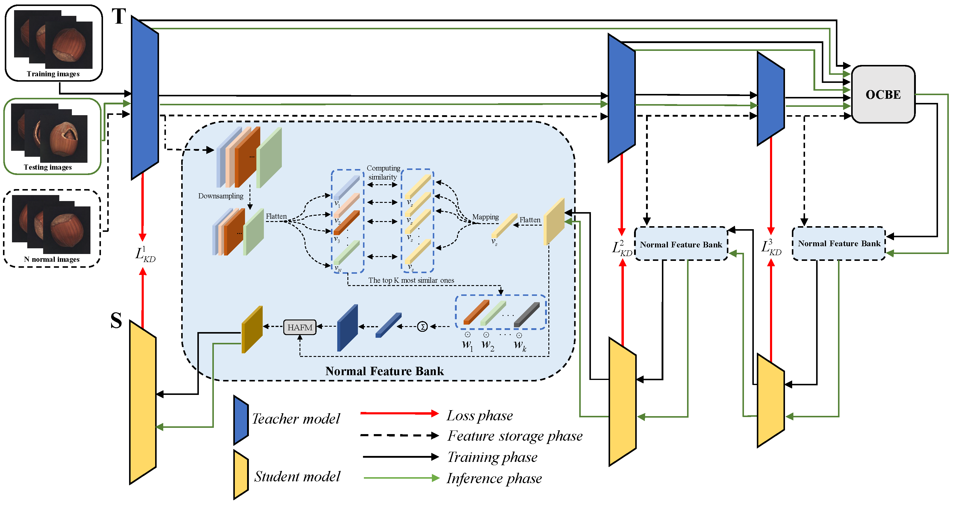
We designed an efficient network framework called Normal Feature-Enhanced Reverse teacher–student Distillation (NFERD) specifically for industrial anomaly detection. As shown in Figure 2, NFERD consists of three core components: a reverse knowledge distillation network, normal feature bank (NFB), and Hybrid Attention Fusion Module (HAFM). The reverse knowledge distillation network includes a teacher model T and a student model S, both of which use the Wide ResNet50 architecture. Among them, the teacher model was pre-trained on the ImageNet dataset, while the student model was trained from scratch. Our goal was to train the student model to mimic the output of the teacher model. As we point out in the Introduction Section, there is a problem of “feature leakage” in the reverse knowledge distillation network, which may result in some normal areas being incorrectly identified as anomalies. To address this issue, we introduce the normal feature bank, which aims at enhancing the student model’s ability to represent normal features, thereby improving the overall anomaly detection accuracy.

Specifically, we designed three NFBs with the same structure, each of which stores normal feature maps extracted by the teacher model at different stages of the network. The feature maps at each stage represent information at different levels of abstraction. We aimed to fuse normal features from the NFB with those extracted by the student model. This allows the student model to not only learn normal feature representations imparted by the teacher but also directly obtain normal features stored in the NFB, thereby strengthening its representation capabilities for normal features. However, how to fuse the feature maps extracted by the student model with those picked up from the NFB is also a challenge. Therefore, we designed a Hybrid Attention Fusion Module (HAFM), which ensures that key spatial details are preserved while maintaining information between channels during the fusion process by processing spatial attention and channel attention in parallel. The specific implementation of NFERD is as follows: Before the model training, we first randomly selected N normal images from the training dataset and input these images into the pre-trained teacher model. Then, we stored the normal feature maps extracted by the teacher model at different stages of the network in the corresponding NFB. During the model training, the defect-free training images were input into a pre-trained teacher model, which extracted feature maps from three different stages of the model. Then, the OCBE module fused these feature maps from three different stages and input the fused feature map into the student model that was structurally opposite to the teacher model. At the same time, the student model could access these NFBs. Afterward, the feature maps extracted by the teacher model at different stages were subjected to loss calculation with those extracted by the students at the corresponding stages. The following subsection provides a detailed introduction to each module.

3.2. Normal Feature Bank Module

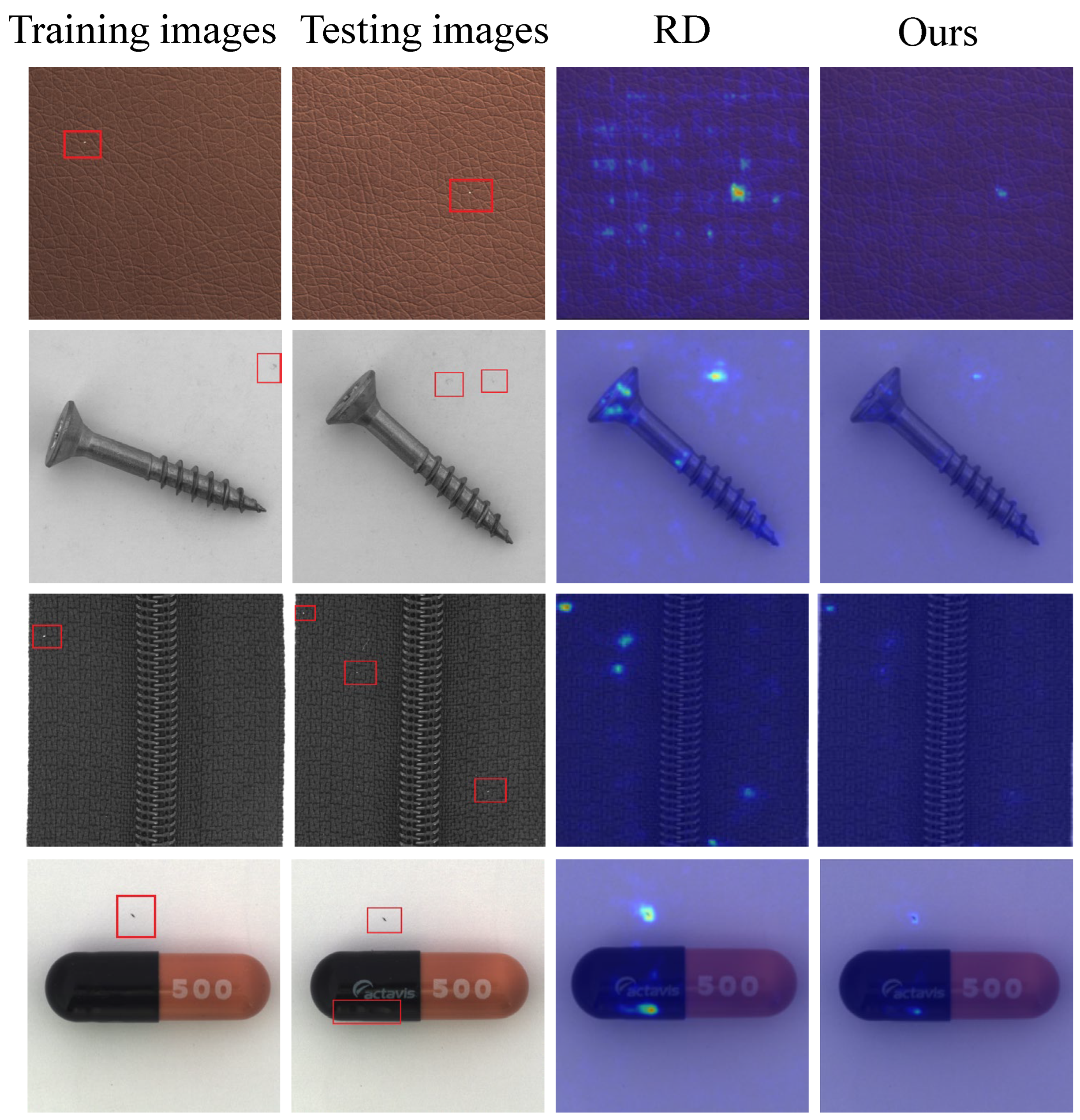
We observed a phenomenon in the reverse knowledge distillation model, i.e., “feature leakage”, which may result in normal areas being incorrectly identified as anomaly areas. To address this issue, we introduced the NFB module, which stored some normal features extracted by the teacher model so that the student model could better learn the normal features. First, we randomly selected N normal samples from the training set, which were then input into the pre-trained teacher model. The teacher model processed these samples and generated feature maps within its four different stages. The feature maps from the first three stages were used for the subsequent NFB storage and network training, while the last stage was used to construct the one-class bottleneck embedding (OCBE) block, which was used to fuse the feature maps from the first three stages. To this end, we created three NFBs with the same structure, each dedicated to storing feature maps extracted by the teacher model at different stages. Before storing the feature maps in the NFB, the feature maps were first downsampled through bilinear interpolation to adjust their sizes, ensuring that each size matched the output of the student model in the corresponding stage. Then, we adjusted the number of channels in each feature map through a 1 × 1 convolution operation to match the number of channels extracted by the student model in the corresponding stage.

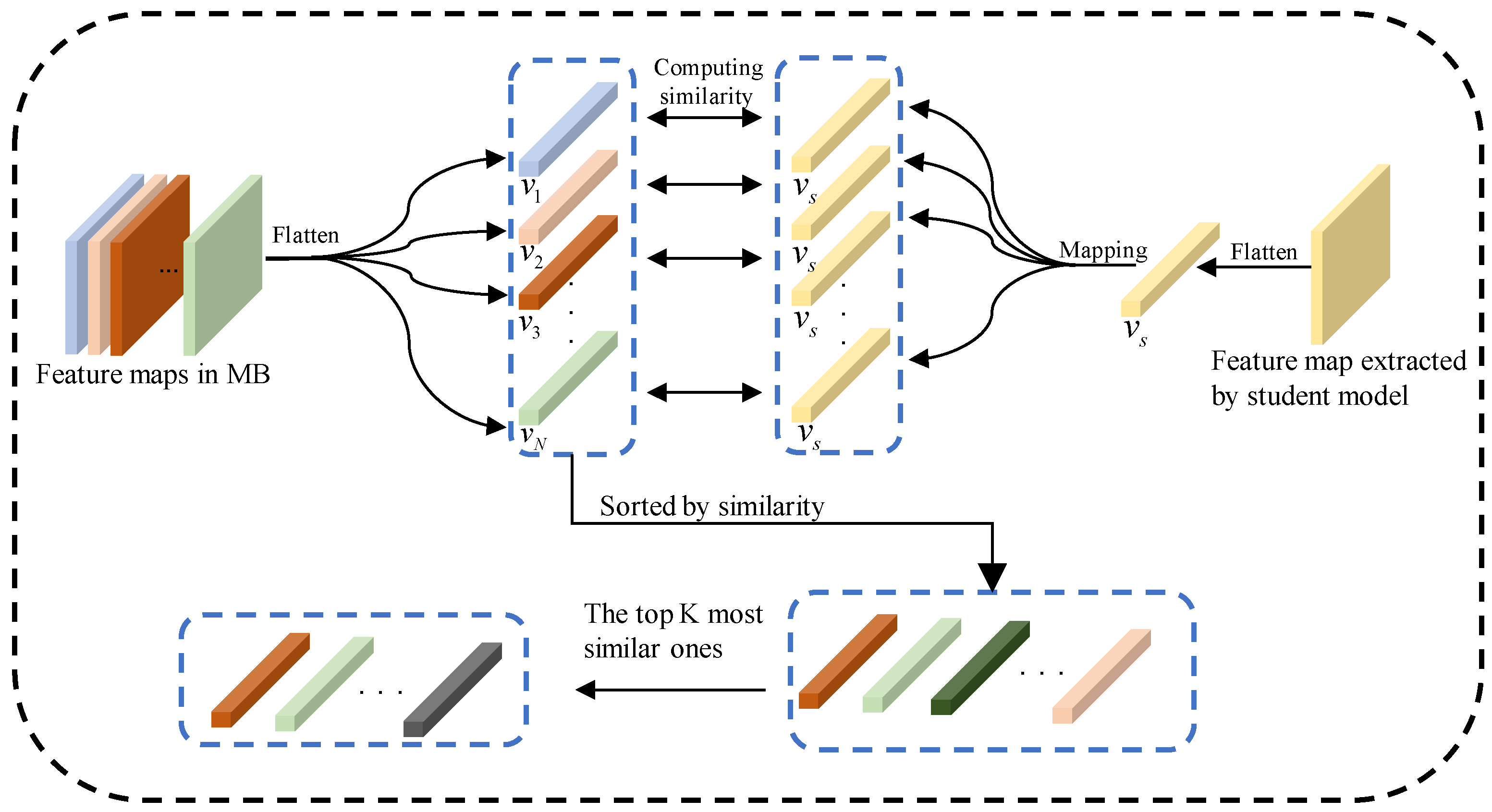
In the student model stage, we hoped to fuse the feature maps extracted by the student model with those in the NFBs. For optimal utilization, we assessed the similarity between the student’s feature maps and all NFB feature maps. Specifically, we flattened the feature maps in NFBs and the feature maps extracted by the student model into one-dimensional vectors to calculate their similarity. The specific steps were as follows: First, we flattened N feature maps stored in the NFBs into one-dimensional vectors and recorded them as $v_1,v_2,\dots ,v_N$. A similar flattening operation was also applied to the feature map extracted by the student model and recorded as $v_s$. Then, we calculated the cosine similarity between $v_s$ and $v_1,v_2,\dots ,v_N$ separately, to obtain the similarity set S. In this way, we could quantify the similarity between the features extracted by the student model and the features stored in the NFBs. Note that $S_i$ represents the similarity between the feature map extracted by the student model and the i-th feature map in the NFB. The similarity $S_i$ and similarity set S can be calculated by the following formula:

$$S_i(v_s,v_i)={\displaystyle \frac{v_s·v_i}{∥v_s∥∥v_i∥}},$$

(1)

$$S=\left\{S_i(v_s,v_i),i=1,2,\dots ,N\right\}.$$

(2)

Feature maps with a high similarity usually contain information similar to the feature maps extracted by the student model, which means that these feature maps are more likely to contain information that is more useful for the learning of the student model. In contrast, feature maps with a lower similarity may contain different or irrelevant information, and using this information may interfere with the learning process of the student models. If the similarity between the vector $v_s$ and vectors $v_1,v_2,\dots ,v_N$ is low, excluding these vectors is advisable, as they may not contain relevant normal feature information. Therefore, we selected K vectors with the highest similarity from $v_1,v_2,\dots ,v_N$. Specifically, we sorted the similarity set S from high to low to obtain the similarity set $S_{sorted}$. Then, we selected the top K vectors from $S_{sorted}$ to obtain the similarity subset $S_k$. The process of obtaining the top K most similar ones is shown in Figure 3.

$$S_{sorted}=\left\{S_1(v_s,v_1),S_2(v_s,v_2),\dots ,S_N(v_s,v_N)\right\},$$

(3)

$$S_k=\left\{S_1(v_s,v_1),S_2(v_s,v_2),\dots ,S_K(v_s,v_K)\right\}.$$

(4)

To enable the student model to obtain more valuable information from the NFB, thereby improving the learning effectiveness and model performance, we calculated the corresponding weight w for the similarity set $S_k$, which represents how many relevant normal features need to be recalled from the corresponding feature maps. The main purpose of introducing weight w was to ensure that the student model could focus on extracting the most valuable information from the NFB, thereby optimizing the distillation process. By aggregating the weight and corresponding feature vector, the final weighted feature vector recalled from the NFB could be obtained. The weighted feature vector was then reshaped into a weighted feature map and returned to the student model. The weight w and the final returned feature vector v could be calculated using the following specific formula:

$$w_i={\displaystyle \frac{S_i}{{\sum }_{j=1}^K{S}_j}},$$

(5)

$$v=\sum _{i=1}^K{w}_i·v_i.$$

(6)

3.3. Hybrid Attention Fusion Module

How to fully utilize these feature maps in NFBs is also an important challenge. Although adding feature maps directly or concatenating them by channel is a common feature fusion method, direct addition may result in information loss, while concatenating them by channel may cause problems of dimensionality expansion and redundant information. 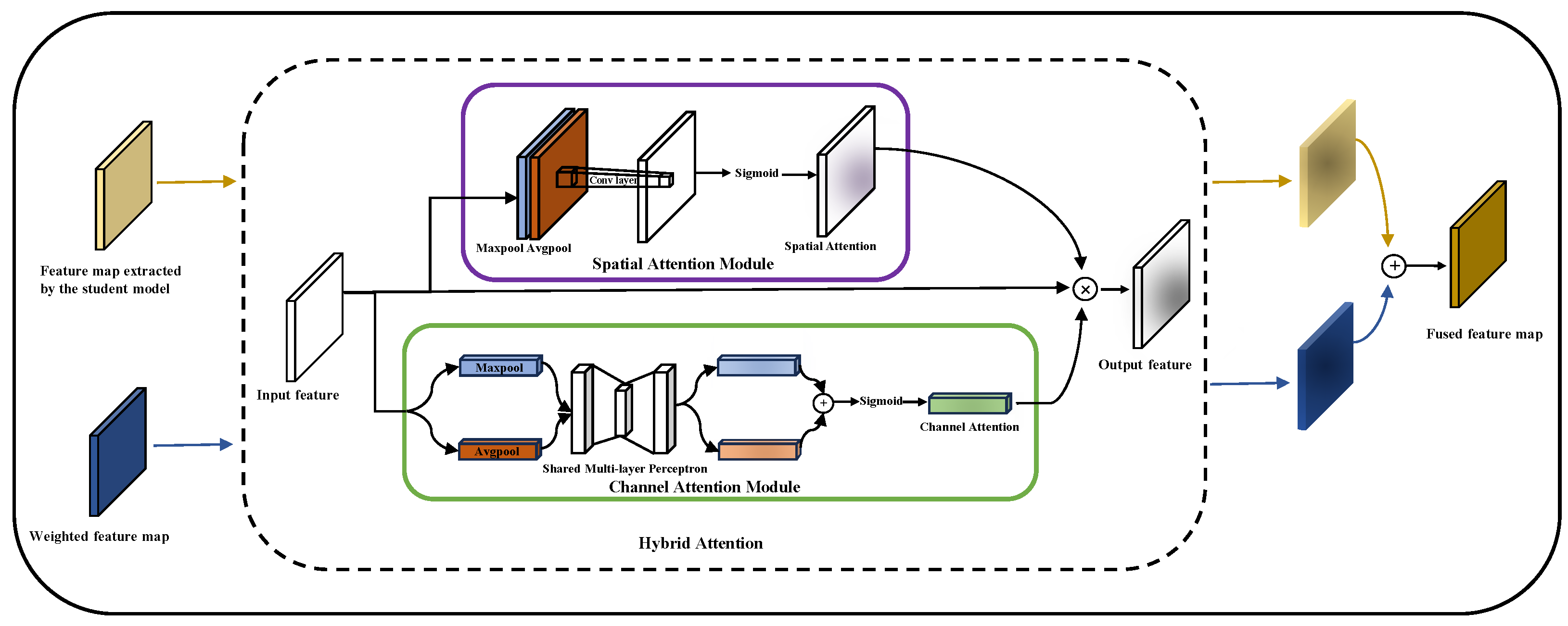In addition, a Convolutional Block Attention Module (CBAM) [23] sequentially processes the Channel Attention Module (CAM) and Spatial Attention Module (SAM) through concatenation. This serial processing means that the input of the latter module depends on the output of the previous module. In deep network architectures, this serial processing order may cause delays or information loss during transmission. To overcome these limitations, we designed a Hybrid Attention Fusion Module (HAFM), which parallelizes the spatial attention and channel attention to ensure that key spatial details are preserved and inter-channel information is maintained during the fusion process. The designed HAFM is shown in Figure 4. Specifically, in the HAFM, the spatial attention mechanism is used to capture important regions in the feature map, emphasizing or suppressing feature responses at certain spatial positions by learning a weight matrix. Meanwhile, the channel attention mechanism focuses on the interdependence between different feature channels, assigning a weight to each channel to highlight the more critical features of the task. The parallel processing of these two attention mechanisms will result in a more robust and informative feature representation. Through this, the HAFM can effectively integrate feature information from different sources, providing more refined and targeted feature representations for subsequent task processing.

3.4. Loss Function

Cosine similarity is an effective method for measuring the similarity between feature maps. It is widely used in various applications. In this study, we used cosine similarity to measure the similarity between the output feature maps of the teacher model and the student model. Specifically, we used $F_T^i$ to represent the output feature map of the teacher model in the i-th stage of the network, and $F_S^i$ to represent the output feature map of the student model in the same stage. Our training objective was to make the output feature map of the student model as close as possible to the output feature map of the teacher model. Therefore, the two-dimensional anomaly score graph $M^i$ in the i-th stage could be calculated using the following formula:

$$M^i(x,y)=1-{\displaystyle \frac{{\left(F_T^i(x,y)\right)}^T·(F_S^i(x,y))}{∥\left(F_T^i(x,y)\right)∥∥F_S^i(x,y))∥}},$$

(7)

where $(x,y)$ represents the spatial position in the feature map. When the value of $M^i$ is large, it indicates that the similarity between the feature map $F_T^i$ and $F_S^i$ at position $(x,y)$ is small. Given that the teacher model and student model output feature maps at multiple stages, the distillation loss function $L_{KD}$ that guides the optimization of the student model can be defined as

$$L_{KD}=\sum _{i=1}^I\left({\displaystyle \frac{1}{X_i{Y}_i}}\sum _{x=1}^{X_i}\sum _{y=1}^{Y_i}{M}^i(x,y)\right),$$

(8)

where $X_i$ and $Y_i$, respectively, represent the width and height of the feature map output by the network in the i-th stage, and I represents the number of feature maps output by the network and was set to three in this paper.

4. Experimental Results and Discussions

In this section, we evaluate the anomaly detection and localization performance of our NFERD method on the MVTec dataset [24] and Kolektor Surface-Defect Dataset (KSDD) [25] using several evaluation metrics.

4.1. Datasets

MVTec dataset: The MVTec dataset is a widely used dataset specifically designed for anomaly detection research. It contains 5354 high-resolution color images. These images are divided into 15 different object and texture categories.

KSDD: The KSDD is a publicly available dataset for surface defect detection, consisting of 52 images with visible defects and 347 images without defects, with an image size of 230 × 630 pixels. We used a three-fold cross-validation strategy, using only the anomaly-free images to evaluate the performance of the model.

4.2. Evaluation Metrics

Image-level anomaly score: To evaluate the overall performance of anomaly detection on an image level, we utilized the Area Under the Receiver Operating Characteristic Curve (AUROC). This metric provides a comprehensive measure of how well a model can distinguish between normal and anomalous images. The AUROC score ranges from 0 to 1, where a higher value indicates better discrimination ability.

Pixel-level anomaly score: To assess the precision of anomaly localization at the pixel level, we employed two metrics: the AUROC and the Per-Region-Overlap (PRO) score [20]. The AUROC was again used here to evaluate the model’s capability in distinguishing between normal and anomalous pixels. The PRO, on the other hand, quantifies the overlap between detected anomalies and true anomalies on a per-region basis, which is particularly useful for understanding the spatial accuracy of the detection.

4.3. Experimental Settings

In our network architecture, both the teacher encoder and the student decoder utilize Wide ResNet50 as the base network. Wide ResNet [26,27,28], an enhancement over the original ResNet architecture by increasing the network width, has been widely utilized. Notably, the teacher encoder was pre-trained on the ImageNet [29] dataset, while the student network was designed in the opposite direction to the teacher’s architecture. The number N of feature maps stored in the normal feature bank (NFB) was set to 20. The input image dimensions varied depending on the dataset: 256 × 256 for the MVTec dataset and 704 × 256 for the KSDD. Our network was trained for 200 epochs with a batch size of four. The learning rate was set to 0.005 for both the MVTec dataset and the KSDD. The Adam optimizer [30] was employed with parameters ${\beta }_1=0.5$ and ${\beta }_2=0.999$. Our framework was implemented using PyTorch 1.10.1 and trained on an NVIDIA RTX 3090 Ti GPU. For comparative methods, we configured the hyper-parameters according to the recommendations provided in their original publications.

4.4. Experimental Results on the MVTec Dataset

In this experiment, we chose Spade [15], US [20], MKD [19], PaDiM [16], PatchCore [17], RD [4], and HFRA [31] as the baselines and present a detailed comparison of our proposed method with other mainstream methods using three metrics in

Table 1. Anomaly detection results in terms of the I-AUROC on the MVTec dataset.

Category/Method		Spade [15]	US [20]	MKD [19]	PaDiM [16]	PatchCore [17]	RD [4]	HFRA [31]	Ours
Texture	Carpet	92.80	91.60	79.30	99.80	98.70	98.90	100	99.96
	Grid	47.30	81.00	78.00	96.70	98.20	100	98.80	100
	Leather	95.40	88.20	95.10	100	100	100	100	100
	Tile	96.50	99.10	91.60	98.10	98.70	99.30	98.60	99.57
	Wood	95.80	97.70	94.30	99.20	99.20	99.20	98.60	99.30
	Avg	85.56	91.52	87.66	98.76	98.96	99.48	99.20	99.77
Object	Bottle	97.20	99.00	99.40	99.90	100	100	100	100
	Cable	84.80	86.20	89.20	92.70	99.50	95.00	98.90	98.13
	Capsule	91.00	86.10	80.50	91.30	98.10	96.30	93.60	98.88
	Hazelnut	88.10	93.10	98.40	92.00	100	99.90	100	100
	Metal nut	71.00	82.00	73.60	98.70	100	100	99.90	100
	Pill	80.10	87.90	82.70	93.30	96.60	96.60	97.70	98.15
	Screw	66.70	54.90	83.30	85.80	98.10	97.00	96.00	99.26
	Toothbrush	88.90	95.30	92.20	96.10	100	99.50	98.30	99.72
	Transistor	90.30	81.80	85.60	97.40	100	96.70	99.70	98.25
	Zipper	96.60	91.90	93.20	90.30	99.40	98.50	98.60	98.58
	Avg	85.47	85.82	87.81	93.75	99.17	97.95	98.27	99.10
Total avg		85.50	87.72	87.76	95.42	99.10	98.46	98.60	99.32

,

Table 2. Anomaly localization results in terms of the P-AUROC on the MVTec dataset.

Category/Method		Spade [15]	US [20]	MKD [19]	PaDiM [16]	PatchCore [17]	RD [4]	HFRA [31]	Ours
Texture	Carpet	97.50	93.50	95.64	99.10	99.00	98.90	98.90	99.02
	Grid	93.70	89.90	91.78	97.30	98.70	99.30	98.30	99.35
	Leather	97.60	97.80	98.05	99.20	99.30	99.40	99.10	99.42
	Tile	87.40	92.50	82.77	94.10	95.40	95.60	95.10	96.38
	Wood	88.50	92.10	84.80	94.90	95.00	95.30	96.20	95.50
	Avg	92.94	93.16	90.61	96.92	97.48	97.70	97.52	97.93
Object	Bottle	98.40	97.80	96.32	98.30	98.60	98.70	97.80	98.58
	Cable	97.20	91.90	82.40	96.70	98.40	97.40	97.50	97.91
	Capsule	99.00	96.80	95.86	98.50	98.80	98.70	98.20	98.83
	Hazelnut	99.10	98.20	94.62	98.20	98.70	98.90	98.40	99.14
	Metal nut	98.10	97.20	86.38	97.20	98.40	97.30	97.20	97.75
	Pill	96.50	96.50	89.63	95.70	97.40	98.20	97.40	99.12
	Screw	98.90	97.40	95.96	98.50	99.40	99.60	99.00	99.67
	Toothbrush	97.90	97.90	96.12	98.80	98.70	99.10	98.30	99.15
	Transistor	94.10	73.70	76.45	97.50	96.30	92.50	95.70	95.88
	Zipper	96.50	95.60	93.90	98.50	98.80	98.20	97.70	98.64
	Avg	97.57	94.30	90.76	97.79	98.35	97.86	97.72	98.47
Total avg		96.03	93.92	90.71	97.50	98.06	97.81	97.70	98.29

and

Table 3. Anomaly localization results in terms of the PRO on the MVTec dataset.

Category/Method		Spade [15]	US [20]	MKD [19]	PaDiM [16]	PatchCore [17]	RD [4]	HFRA [31]	Ours
Texture	Carpet	94.70	87.90	-	96.20	96.60	97.00	95.20	97.31
	Grid	86.70	95.20	-	94.60	96.00	97.60	94.40	97.77
	Leather	97.20	94.50	-	97.80	98.90	99.10	97.60	99.15
	Tile	75.90	94.60	-	86.00	87.30	90.60	79.80	92.14
	Wood	87.40	91.10	-	91.10	89.40	90.90	90.80	93.26
	Avg	88.38	92.66	-	93.14	93.64	95.04	91.56	95.93
Object	Bottle	95.50	93.10	-	94.80	96.20	96.60	92.10	96.12
	Cable	90.90	81.80	-	88.80	92.50	91.00	92.60	92.91
	Capsule	93.70	96.80	-	93.50	95.50	95.80	90.50	96.38
	Hazelnut	95.40	96.50	-	92.60	93.80	95.50	97.60	96.28
	Metal nut	94.40	94.20	-	85.60	91.40	92.30	99.40	92.76
	Pill	94.60	96.10	-	92.70	93.20	96.40	94.70	97.85
	Screw	96.00	94.20	-	94.40	97.90	98.20	95.00	98.78
	Toothbrush	93.50	93.30	-	93.10	91.50	94.50	86.50	94.72
	Transistor	87.40	66.60	-	84.50	83.70	78.00	88.50	86.83
	Zipper	92.60	95.10	-	95.90	97.10	95.40	93.10	96.18
	Avg	93.40	90.77	-	91.59	93.28	93.37	93.00	94.88
Total avg		91.73	91.40	-	92.11	93.40	93.93	92.50	95.23

. These metrics were the Image-level AUROC (I-AUROC), Pixel-level AUROC (P-AUROC), and PRO score (PRO). Table 1 shows the results of our method on the I-AUROC. From the data, it can be seen that our method achieved an average performance of 99.32% in 15 categories, which was 0.22% higher than the second-best result and demonstrated significant advantages. It is worth mentioning that our method achieved the best level in different texture categories, which strongly proved our method’s excellent ability to handle anomaly detection in texture categories. Table 2 and Table 3 show the pixel-wise anomaly localization results of our method. It is evident from the tables that our method demonstrated excellent performance in all three metrics. In 15 different categories, our method achieved an average P-AUROC and PRO of 98.29% and 95.23%, respectively. Compared with the second-best results, the improvements were 0.48% and 1.3%, respectively. This further demonstrated its powerful ability for anomaly localization. Furthermore, compared with RD, our method demonstrated a higher anomaly localization performance. This also fully demonstrated the significant advantages of combining the reverse knowledge distillation with the normal feature bank.

From Figure 5, it can be seen that our method showed significant differences in the visualization effects compared with the RD methods. Specifically, in the third and fourth rows of the figure, there was a sharp contrast between the RD method and our method. The RD method was obviously susceptible to the influence of surrounding noise, which led to poor performance in defect segmentation. In contrast, our method demonstrated superior visualization performance, accurately segmenting the defect area completely while effectively avoiding interference from the surrounding noise areas.

4.5. Experimental Results on the KSDD

In this experiment, we selected six methods for comparative analysis: US [20], PaDim [16], PatchCore [17], Semi-Orthogonal (SO) [32], GMFF [33], and RD [4]. Following [32,34,35], we employed a three-fold cross-validation strategy to evaluate the performance of these methods.

Table 4. Anomaly localization results in terms of the P-AUROC on the KSDD, where we report the average value (Avg) and standard deviation (Std) of each fold.

Method	US [20]	PaDim [16]	PatchCore [17]	SO [32]	GMFF [33]	RD [4]	Ours
Fold1	90.40	93.90	93.30	95.30	96.20	97.86	97.90
Fold2	88.30	93.50	93.40	95.10	98.16	98.67	98.92
Fold3	90.20	96.20	93.90	97.60	98.32	99.03	99.43
Avg ± Std	89.63 ± 1.20	94.53 ± 1.50	93.53 ± 0.15	96.00 ± 1.40	96.80 ± 0.00	98.52 ± 0.44	98.75 ± 0.74

presents the P-AUROC results, from which we can see that our method exhibited significant performance advantages. Specifically, in the results of Fold1 and Fold2, our method improved by 0.04% and 0.25%, respectively, compared with the second-best results. This advantage was more prominent in Fold3, with an improvement of 0.4% compared with the second-best result. When calculating the average performance of all the folds, our method outperformed the second-best method by 0.25%. Figure 6 provides visual results that intuitively demonstrate the performance of our method and other comparative methods. It can be clearly seen from the first line that the KSDD had complex background noise, which posed a great challenge during the defect detection tasks. These complex backgrounds not only increase the difficulty of detection but may also introduce additional noise that interferes with the model’s accurate identification of actual defects. As shown in the third line of the figure, the PatchCore method was susceptible to the influence of the surrounding noise, which resulted in the defect area not being correctly segmented. In contrast, the RD method (fourth line) and our method (fifth line) showed better visualization results and were able to completely segment the defect area. However, it is also evident from the figure that RD was also susceptible to the influence of complex backgrounds, which resulted in many non-defective areas being incorrectly labeled. In contrast, our method performed better in handling complex backgrounds, which effectively avoided mislabeling non-defective areas as anomalies and ensured more accurate segmentation results.

4.6. Ablation Study

Effect of the number of fused feature maps on the model performance: The number of fused feature maps from the NFB may affect the performance of the model, as it determines the richness of the feature information accessible to the model. Inadequate fusion may lead to information scarcity, potentially affecting the accuracy of the model. Conversely, excessive fusion may introduce redundant information, noise, and unnecessary computational burdens. Therefore, in this part, we delve into the impact of fusing different numbers of feature maps from the NFB on the model performance. Through an experimental analysis of the MVTec dataset and the KSDD, we evaluated the performance of the model when the number of fused feature maps was 0, 5, 10, 15, 20, and 25. When the number of fused feature maps was 0, the model degenerated into the baseline method (RD [4]). From the experimental results in

Table 5. Comparison of the anomaly detection and localization performance of 15 categories via fusing different numbers of feature maps on the MVTec dataset.

Number	0	5	10	15	20	25
I-AUROC	98.46	99.08	99.19	99.13	99.32	98.81
P-AUROC	97.81	98.20	98.22	98.09	98.26	98.23
PRO	93.93	95.08	95.08	94.92	95.23	95.06

and

Table 6. Performance comparison in terms of the P-AUROC via fusing different numbers of feature maps on the KSDD.

Number	0	5	10	15	20	25
Fold1	97.86	97.89	97.81	97.89	97.90	97.80
Fold2	98.67	98.31	98.63	98.38	98.92	98.56
Fold3	98.52	99.33	99.42	98.91	99.43	99.42
Avg	98.35	98.51	98.62	98.39	98.75	98.59

, it can be seen that all cases where the number of fused feature maps was greater than 0 exhibited better performance compared with the case where the number of fused feature maps was 0 (RD), which strongly proved the effectiveness of our propose NFERD method in the anomaly detection tasks. Furthermore, from Table 5, it can be observed that when the number of fused feature maps was 20, the I-AUROC, P-AUROC, and PRO all reached their highest levels. Similar results can be obtained from Table 6; when the number of fused feature maps was set to 20, the P-AUROC reached the best value. It is worth noting that when the number of feature maps reached 25, these metrics stopped improving, which indicates that the number of fused feature maps was not simply a case of “the more, the better”, but rather there existed an optimal balance point for the selected datasets. In this paper, we set the number of fused feature maps to 20.

Effect of different feature fusion strategies on the model performance: As discussed in this section, we investigated the effectiveness of the Hybrid Attention Fusion Module (HAFM) in the anomaly detection tasks. Specifically, we compared the impact on the model performance by replacing the HAFM with simple fusion mechanisms, i.e., adding feature maps directly (adding) or concatenating by channel (CC). Furthermore, to validate the effectiveness of our designed HAFM with a parallel processing strategy, we also conducted two additional experiments: one by replacing the HAFM with a single Channel Attention Module (CAM) and Spatial Attention Module (SAM) independently, and the other by modifying the parallel mechanism in the HAFM into a serial processing mechanism of the SAM and CAM (SAM + CAM or CAM + SAM). These experiments were conducted on the MVTec dataset and the KSDD. The experimental results are shown in

Table 7. Anomaly detection and localization results of different fusion strategies on the MVTec dataset.

Fusion Strategies	I-AUROC	P-AUROC	PRO
Adding	98.79	97.94	94.57
CC	98.22	97.84	94.61
SAM	98.96	97.89	94.60
CAM	99.01	97.97	95.02
SAM + CAM	96.28	97.51	93.30
CAM + SAM	91.61	95.69	88.94
HAFM	99.32	98.29	95.23

and

Table 8. Anomaly localization result of different fusion strategies in terms of the P-AUROC on the KSDD.

Fusion Strategies	Fold1	Fold2	Fold3	Avg
Adding	97.85	98.73	99.27	98.62
CC	97.39	98.71	99.06	98.39
SAM	97.70	98.68	98.70	98.36
CAM	97.64	98.80	99.06	98.50
SAM + CAM	97.86	98.83	99.13	98.61
CAM + SAM	97.47	98.71	99.25	98.48
HAFM	97.90	98.92	99.43	98.75

. First, on the MVTec dataset, when using simple fusion strategies, i.e., adding (the first row) and CC (the second row), the I-AUROC, P-AUROC, and PRO reached 98.79%, 97.94%, and 94.57%, and 98.22%, 97.84%, and 94.61%, respectively. When only the SAM (the third row) or CAM (the fourth row) was used for the feature fusion, the I-AUROC, P-AUROC, and PRO reached 98.96%, 97.89%, and 94.60%, and 99.01%, 97.97%, and 95.02%, respectively. It is worth noting that when processing the attention modules in series, the values of the three metrics decreased significantly (fifth and sixth rows). Our HAFM, which processes the CAM and SAM in parallel, produced the highest performance in terms of all these three metrics, showing significant improvement compared with the other fusion strategies. Similar observations were also found on the KSDD. These results strongly confirm the superiority of the HAFM in feature fusion and its positive impact on the model performance.

5. Conclusions

We propose an unsupervised anomaly detection method called NFERD. The core innovation of NFERD lies in the combination of reverse knowledge distillation technology and the normal feature bank (NFB) mechanism, aiming to improve the representation ability of student models on normal sample features. Specifically, the NFB is used to store normal feature maps extracted by the teacher model at different stages of the network, which are then used as reference learning for the student model. To reduce information loss and redundancy issues caused by simple fusion mechanisms, i.e., adding feature maps directly or concatenating them by channel and effectively fusing the feature maps extracted by the student model with those stored in the NFB, we designed a Hybrid Attention Fusion Module (HAFM). It processes spatial attention and channel attention in parallel to ensure that key spatial details are preserved and inter-channel information is maintained during the fusion process. Comparative experiments and ablation studies conducted on two publicly available datasets confirmed the effectiveness and superiority of the proposed method.