The Study of an Improved Particle Swarm Optimization Algorithm Applied to Economic Dispatch in Microgrids

Abstract

With the widespread use of fossil fuels, the Earth’s environment is facing a severe threat of degradation. Traditional large-scale power grids have struggled to meet the ever-growing demands of modern society. The implementation and functioning of microgrids not only enhance the use of renewable energy sources but also considerably diminish the environmental damage resulting from fossil fuel consumption. However, the inherent instability of renewable energy presents a major challenge to the reliability of microgrids. To address the uncertainties of wind and photovoltaic power generation, it is urgent to adopt effective operational control methods to adjust power distribution, thereby achieving an economically efficient system operation and ensuring a reliable power supply. This paper utilizes a microgrid system consisting of wind power, photovoltaic power generation, thermal power units, and energy storage devices as the research object, establishing an economic dispatch model aimed at minimizing the total operating cost of the system. To solve this problem, the paper introduces second-order oscillatory particles and improves the Particle Swarm Optimization algorithm, proposing a second-order oscillatory chaotic mapping particle swarm optimization (SCMPSO). The simulation results show that this method can effectively optimize system operating costs while ensuring the stable operation of the microgrid.

1. Introduction

1.1. Background

As society continues to progress, there is a consistent rise in global energy demands. However, the extensive use of traditional fossil fuels inevitably triggers global energy and environmental crises [1]. In response to these challenges, the widespread application of renewable energy has become an effective approach, as it reduces reliance on fossil fuels and mitigates the negative impact of energy consumption on the environment. The exploration of clean energy has steadily progressed, with the efficient and safe utilization of these resources emerging as a key area of research today. To further utilize these renewable energy sources more efficiently, microgrids, a new type of small-scale power network, have become a research hotspot. The emergence of microgrids has made the efficient utilization of renewable energy possible.

As a new type of power operation model that includes distributed renewable energy, microgrids offer unique advantages. They are flexible and adaptable in power generation and can effectively regulate energy exchanges between the microgrid and the main grid [2]. However, microgrids also face notable challenges, particularly the volatility and uncontrollability of wind and photovoltaic (PV) power generation, which pose significant challenges to their use within microgrids. It is essential to thoroughly analyze the output uncertainties of wind and solar power and optimize dispatch strategies to enable the complementarity of various energy sources [3]. Reference [3] proposes a distributed optimization algorithm for the dynamic economic dispatch problem, aiming to minimize generation costs, and analyzes it within the context of a microgrid model. The model ensures a stable system operation by controlling constraints such as supply–demand balance and generation equipment capacity. The reference uses the weighted sum method to transform the multi-objective optimization problem into a single-objective optimization problem and performs an in-depth analysis of the algorithm’s convergence through a convex analysis and the Lyapunov function method. Reference [4] proposes a sophisticated model predictive control strategy for hybrid energy storage systems. This strategy comprehensively considers the interactions between the hydrogen energy storage system (hydrogen-ESS), the battery energy storage system (battery-ESS), and external loads. The strategy optimizes the system from various aspects, including the economic efficiency and operating costs of the hybrid energy storage system. By employing a mixed-logic dynamic framework, the system is modeled to switch operating modes based on the real-time operational state of the equipment. Additionally, the strategy’s superiority is validated through case simulations. In addition, since diesel generators emit pollutants during operation, reducing fossil fuel consumption in microgrid operations has become a key focus of current research.

1.2. Literature Review

As renewable energy rapidly advances and fossil fuel resources become increasingly scarce, optimizing energy supply systems has become a core topic of current research. Presently, international scholars mainly focus on two areas in microgrid dispatch research: model development and algorithm enhancement.

• Regarding model development: Early studies primarily focused on the stability and economic efficiency of grid operations. Reference [5] explored how to improve the economic efficiency of microgrid operations by leveraging the dispatch characteristics of microgrids while also maintaining grid stability. Reference [6] investigated the coordinated dispatch strategy of large grids and natural gas systems to reduce overall operating costs, with the goal of minimizing fuel costs. Reference [7] proposed an analysis model for microgrid operations with the dual objectives of maximizing economic benefits and minimizing emissions. Reference [8] constructed a model from the perspective of coordinated operation across multiple microgrid systems, aiming to minimize economic costs while ensuring system stability. Additionally, since thermal generators are typically present in microgrids, reducing the use of fossil fuels and lowering pollutant emissions have become closely related optimization objectives. To address multi-objective optimization dispatch issues, researchers often introduce penalty functions to transform multi-objective problems into single-objective ones [9,10,11].
• In terms of algorithm optimization: Research has mainly focused on improving global convergence speed and solution accuracy. Particle Swarm Optimization (PSO) is widely applied to solve power system issues due to its simplicity, easy parameter tuning, and robust global search ability. However, PSO has some limitations, such as susceptibility to local optima and a relatively slow convergence speed [12,13,14]. To address these shortcomings, some scholars have proposed new search strategies to improve the algorithm’s global search performance. Additionally, some researchers have combined PSO with other algorithms, as mentioned in references [15,16,17,18], which has also contributed to improving the global search capability of traditional PSO algorithms.

In summary, there is still considerable room for improvement in both model construction and algorithm optimization. This paper considers additional influencing factors in the model construction, aiming to establish a more comprehensive dispatch model. In terms of algorithm optimization, an improved SCMPSO algorithm is used for optimization and simulation.

The key contributions of this paper are as follows:

(1)

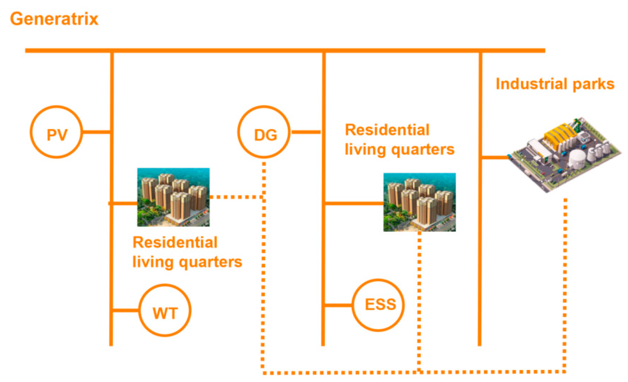
Constructing a dispatch model that includes distributed photovoltaic generation (PV), wind turbines (WT), thermal power generators (DG), and energy storage systems (ESS);

(2)

Introducing second-order oscillatory particles and improving the iteration formula of swarm particles to optimize the traditional PSO algorithm;

(3)

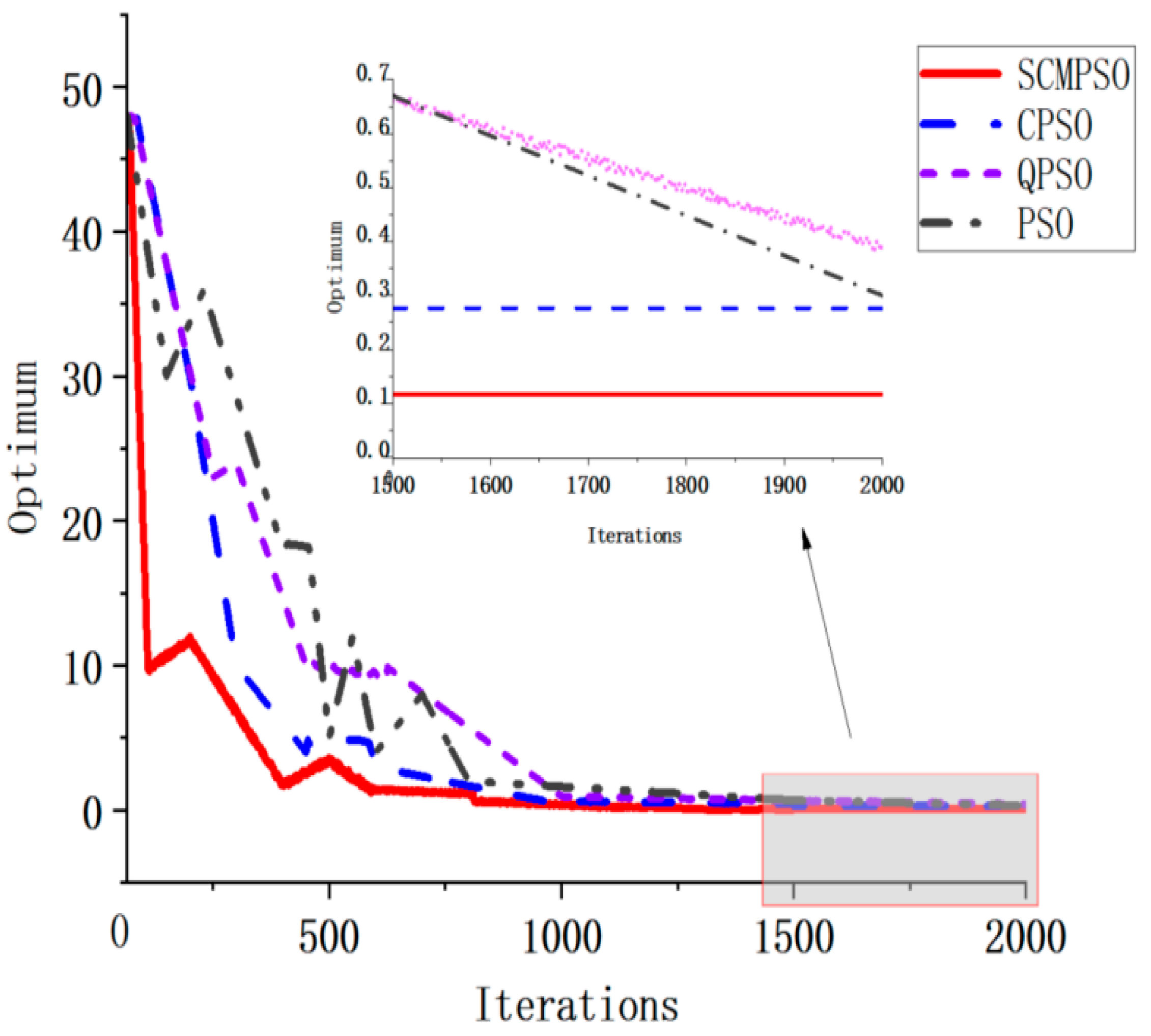
Conducting a comparative analysis of SCMPSO with traditional PSO, Cooperative Particle Swarm Optimization(CPSO), and Quantum-behaved Particle Swarm Optimization (QPSO) to verify the superiority of SCMPSO in optimization performance.

2. Microgrid Model Construction

The microgrid model developed in this paper primarily consists of the following key components: a distributed photovoltaic generation system (PV), wind turbines (WT), small thermal power generators (DG), and an energy storage system (ESS). Ensuring a stable system operation, the paper aims to minimize both operating and environmental costs by establishing an objective function.

2.1. Photovoltaic Model Construction

The photovoltaic (PV) component achieves energy output through photovoltaic modules. Based on the principles of photovoltaic power generation, the energy conversion efficiency of PV systems is significantly influenced by natural conditions. In addition to solar irradiance, temperature is a key factor affecting PV conversion efficiency. Generally, the higher the temperature, the lower the conversion efficiency of the photovoltaic cells [19]. Therefore, when constructing the PV model, both of these factors must be taken into account.

The expression for the PV output power can be represented as:

$${\mathrm{P}}_{\mathrm{P}\mathrm{V}}={\mathrm{P}}_{\mathrm{o}}\times {\displaystyle \frac{{\mathrm{G}}_{\mathrm{I}\mathrm{N}\mathrm{C}}}{{\mathrm{G}}_{\mathrm{S}\mathrm{T}\mathrm{C}}}}\left(1+\mathrm{k}\left({\mathrm{T}}_{\mathrm{c}}-{\mathrm{T}}_{\mathrm{o}}\right)\right)$$

(1)

In Equation (1), the meanings of the symbols are as follows:

• P_PV: Actual output power of the photovoltaic module;
• P_o: Maximum output power under Standard Test Conditions;
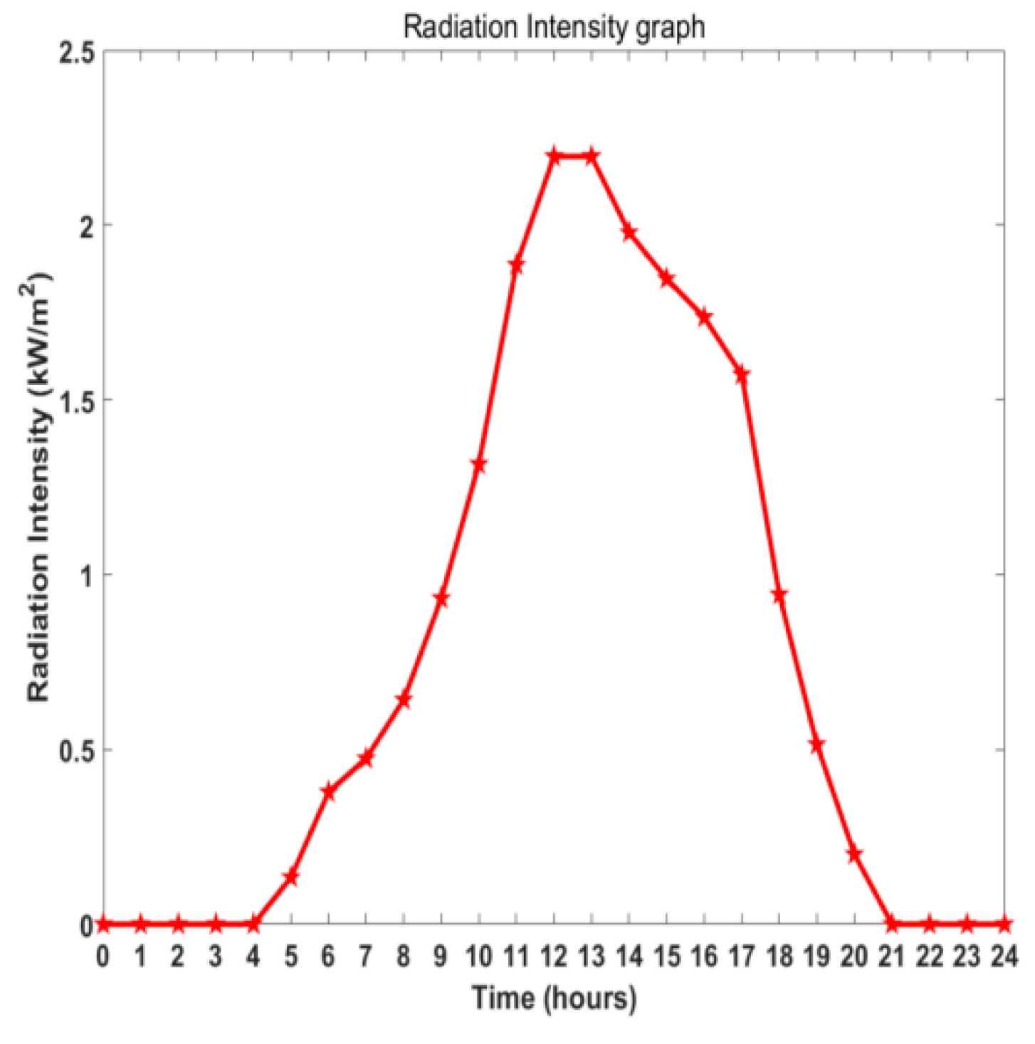
• G_INC: Actual irradiance (in kW/m²);
• G_STC: Irradiance under reference test conditions, set as 1 kW/m²;
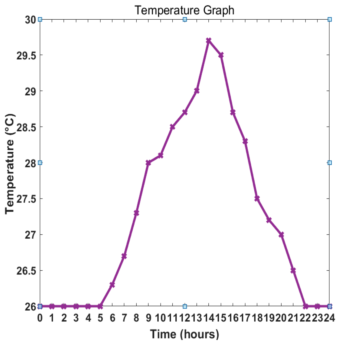
• k: Temperature coefficient of power;
• T_c: Actual operating temperature of the photovoltaic cells;
• T_o: Set operating temperature, typically 25 °C.

2.2. Establishment of Wind-Power Model

A wind turbine’s energy input comes from wind, and the turbine rotor’s rotational speed is governed by the wind speed. The rotor speed is linearly related to the generator speed [20]. The output power of wind generation depends on wind speed and can be described as:

$${\mathrm{P}}_{\mathrm{W}\mathrm{T}}=\left\{\begin{array}{c}0 0\le \mathrm{V}\le {\mathrm{V}}_{\mathrm{i}}\\ {\mathrm{P}}_{\mathrm{r}\mathrm{a}\mathrm{t}\mathrm{e}\mathrm{d}}\times {\displaystyle \frac{\mathrm{V}-{\mathrm{V}}_{\mathrm{i}}}{{\mathrm{V}}_{\mathrm{r}}-{\mathrm{V}}_{\mathrm{i}}}} {\mathrm{V}}_{\mathrm{i}}\le \mathrm{V}\le {\mathrm{V}}_{\mathrm{r}} \\ { \mathrm{P}}_{\mathrm{r}\mathrm{a}\mathrm{t}\mathrm{e}\mathrm{d}} { \mathrm{V}}_{\mathrm{r}} \le \mathrm{V}\le {\mathrm{V}}_{\mathrm{c}} \\ 0 {\mathrm{V}}_{\mathrm{c}} \le \mathrm{V} \end{array} \right.$$

(2)

The symbols in Equation (2) are defined as follows:

• P_WT: Wind turbine output power as a function of wind speed;
• P_rated: Rated output of the wind turbine;
• V: Actual wind speed;
• V_i: The minimum wind speed at which the turbine starts generating power;
• V_r: Rated wind speed, which is the wind speed at which the turbine reaches its rated output power;
• V_c: To ensure equipment safety, the maximum wind speed at which the turbine ceases power generation.

2.3. Establishment of Small Thermal Generator Model

The output power of a thermal generator is mainly related to energy consumption, with the actual output power fluctuating between 30% of the rated power and the actual power [21]. The relationship between fuel consumption and output power of a thermal generator is expressed as:

$${\mathrm{V}}_{\mathrm{F}}(\mathrm{t})={\mathrm{a}}_1\times {\mathrm{P}}_{\mathrm{D}\mathrm{I}\mathrm{E}}(\mathrm{t})+{\mathrm{a}}_2\times {\left({\displaystyle \frac{{\mathrm{P}}_{\mathrm{D}\mathrm{I}\mathrm{E}}\left(\mathrm{t}\right)}{{\mathrm{P}}_{\mathrm{D}\mathrm{G}}\left(\mathrm{t}\right)}}\right)}^2$$

(3)

The symbols in Equation (3) are defined as follows:

• V_F(t): Fuel consumption of the thermal generator at time t, measured in liters (L);
• ${\mathrm{P}}_{\mathrm{D}\mathrm{I}\mathrm{E}}(\mathrm{t})$: Actual output power of the thermal generator at time t, expressed in kilowatts (kW);
• P_DG(t): Rated output power of the thermal generator at time t, given in kilowatts (kW);
• a₁ and a₂: Coefficients of the fuel consumption curve, expressed in liters per kilowatt-hour (L/kWh).

2.4. Establishment of Energy Storage Device Model

The device for energy storage plays a crucial role in ensuring that the microgrid system operates smoothly. When the output power of distributed generation exceeds the load demand, the energy storage device can store the excess electricity. Conversely, when the output power of distributed generation is less than the load demand, the energy storage device can release the previously stored energy. By facilitating this continual cycle of storing and releasing energy, the device contributes to the stable functioning of the grid [22]. The charging and discharging processes of the energy storage device can be expressed as:

$$S_{OC.1}\left(t\right)=(1-\delta )S_{oc}(t-1)+P_c∆t\times {\eta }_c/E_c$$

(4)

$$S_{OC.2}\left(t\right)=(1-\delta )S_{oc}(t-1)-P_d∆t/{(E}_c{\times \eta }_d)$$

(5)

Equation (4) illustrates how the energy storage device charges, while Equation (5) describes the process of discharging. The symbols used are defined as follows:

• $S_{OC}\left(t\right)$: Remaining energy of the storage system at the end of period t;
• $S_{oc}(t-1)$: Remaining energy of the storage system at the end of period t−1;
• $P_c\left(t\right)$ and $P_d\left(t\right)$: Charging and discharging power of the storage system at period t, measured in kilowatts (kW);
• $\delta$: Self-discharge rate of the energy storage device;
• ${\eta }_c$ and ${\eta }_d$: Charging and discharging efficiency of the storage system, measured as a percentage (%);
• $E_c$: Rated capacity of the storage system, measured in kilowatt-hours (kWh).

3. Scheduling Model

3.1. Objective Function

In the study of microgrid economics, minimizing operational costs is the primary economic objective. While guaranteeing that the microgrid system operates reliably, the diverse distributed power sources are efficiently scheduled to lower the overall economic costs. The operational costs of these distributed power sources, along with expenses associated with environmental management and protection, primarily constitute the economic costs of microgrid functioning. The specific objective function is shown as follows:

$$\mathrm{M}\mathrm{i}\mathrm{n}{\mathrm{C}}_{\mathrm{s}\mathrm{u}\mathrm{n}}={\mathrm{C}}_1+{\mathrm{C}}_2$$

(6)

Equation (6) represents the total cost of system operation, which mainly includes system maintenance costs, fuel costs, depreciation costs, and electricity purchase costs. C₂ represents environmental management costs. In a microgrid, both photovoltaic (PV) and wind-power generation are clean energy sources and do not produce pollutants. However, thermal generators emit pollutants such as CO₂, SO₂, and NO_X during operation.

The specific expression for C1 is as follows:

$${\mathrm{C}}_1=\sum _{\mathrm{t}=1}^{\mathrm{T}}\sum _{\mathrm{i}=1}^{\mathrm{N}}({\mathrm{C}}_{\mathrm{i}}^{\mathrm{o}\mathrm{m}}(\mathrm{t})+{\mathrm{C}}_{\mathrm{i}}^{\mathrm{D}\mathrm{G}}(\mathrm{t})+{\mathrm{C}}_{\mathrm{i}}^{\mathrm{D}\mathrm{S}}{ +\mathrm{C}}_{\mathrm{i}}^{\mathrm{g}\mathrm{r}\mathrm{i}\mathrm{d}}(\mathrm{t}))$$

(7)

$${\mathrm{C}}_{\mathrm{i}}^{\mathrm{o}\mathrm{m}}(\mathrm{t})={\mathrm{K}}_{\mathrm{i}}^{\mathrm{P}\mathrm{V}}(\mathrm{t})\times {\mathrm{P}}_{\mathrm{i}}^{\mathrm{P}\mathrm{V}}(\mathrm{t})+{\mathrm{K}}_{\mathrm{i}}^{\mathrm{W}\mathrm{T}}(\mathrm{t})\times {\mathrm{P}}_{\mathrm{i}}^{\mathrm{W}\mathrm{T}}(\mathrm{t})+{\mathrm{K}}_{\mathrm{i}}^{\mathrm{D}\mathrm{G}}(\mathrm{t})\times {\mathrm{P}}_{\mathrm{i}}^{\mathrm{D}\mathrm{G}}(\mathrm{t})+{\mathrm{K}}_{\mathrm{i}}^{\mathrm{E}\mathrm{S}\mathrm{S}}(\mathrm{t})\times {\mathrm{P}}_{\mathrm{i}}^{\mathrm{E}\mathrm{S}\mathrm{S}}(\mathrm{t})$$

(8)

$${\mathrm{C}}_{\mathrm{i}}^{\mathrm{D}\mathrm{G}}(\mathrm{t})={\mathrm{C}}_{\mathrm{r}}\times {\mathrm{P}}_{\mathrm{i}}^{\mathrm{D}\mathrm{G}}(\mathrm{t})/{\mathsf{\eta }}_{\mathrm{i}}^{\mathrm{D}\mathrm{G}}$$

(9)

$${\mathrm{C}}_{\mathrm{i}}^{\mathrm{D}\mathrm{S}}(\mathrm{t})={\mathrm{D}\mathrm{S}}_{\mathrm{i}}\times {\mathrm{P}}_{\mathrm{i}}^{\mathrm{*}}(\mathrm{t})/({\mathrm{p}}_{\mathrm{i},\mathrm{m}\mathrm{a}\mathrm{x}}\times \mathrm{a}\times {\mathrm{f}}_{\mathrm{i}})$$

(10)

$${\mathrm{C}}_{\mathrm{i}}^{\mathrm{g}\mathrm{r}\mathrm{i}\mathrm{d}}(\mathrm{t})={\mathrm{P}}_{\mathrm{c}\mathrm{i}}(\mathrm{t})\times (\mathrm{t})$$

(11)

The symbols used in Equations (7)–(11) are defined as follows:

• C_i^OM(t): Operating and maintenance cost of each device at time t;
• C_i^DG(t): Fuel consumption cost of the thermal generator at time t;
• C_i^grid(t): Interaction cost between the microgrid and the main grid at time t;
• K_i^PV(t), K_i^WT(t), K_i^DG(t), and K_i^ESS(t): Operating and maintenance cost coefficients of the photovoltaic system, wind turbine, thermal generator, and energy storage device at time t, respectively;
• P_i^PV(t), P_i^WT(t), P_i^DG(t), and P_i^ESS(t): Power outputs of the photovoltaic system, wind turbine, thermal generator, and energy storage device at time t, respectively;
• C_i^DG(t): Fuel cost of the thermal generator, where C_r is the fuel price (in CNY/L) and η_i^DG is the efficiency of the thermal generator;
• C_i^DS(t): Depreciation cost of each device, where DS_i is the annual depreciation cost of unit i, and P_i^*(t) is the output power of unit i at time t. P_i,max is the maximum output power of unit i, a is a constant, and f_i is the capacity factor;
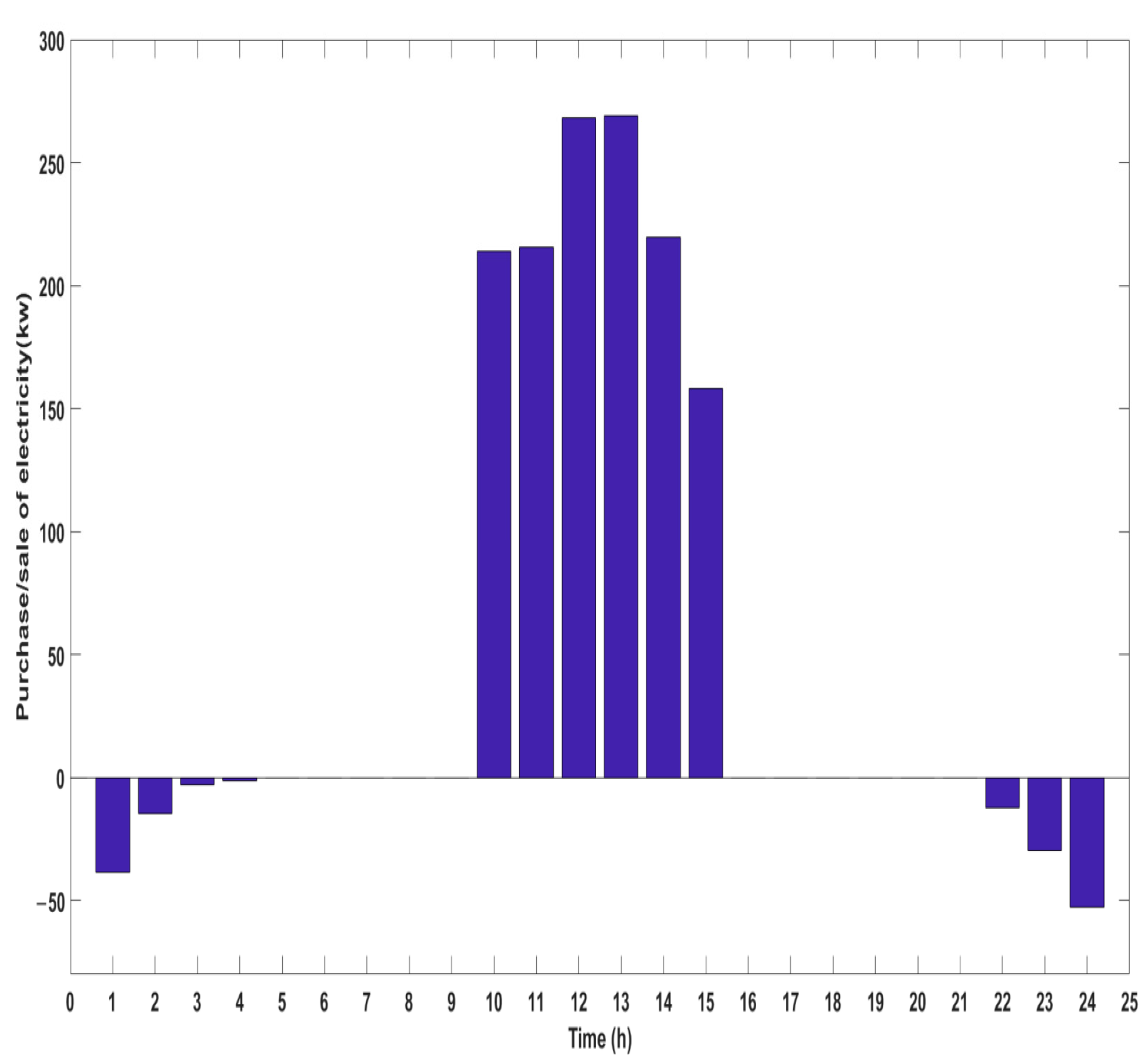
• C_i^grid(t): Interaction cost between the microgrid and the main grid, where P_ci(t) is the amount of electricity purchased from or sold to the main grid at time t, and C_g(t) represents the electricity cost at time t between the main grid and the microgrid.

The specific expression for C₂ is as follows:

$${\mathrm{C}}_2=\sum _{\mathrm{i}=1}^{\mathrm{N}}\sum _{\mathrm{j}=1}^3{\mathrm{l}}_{\mathrm{i},\mathrm{j}}{\mathsf{\lambda }}_{\mathrm{j}}{\mathrm{P}}_{\mathrm{D}\mathrm{I}\mathrm{E}}(\mathrm{t})$$

(12)

Equation (12) defines EP(t) as the amount of pollutant I_i,j emitted by the thermal generator per unit output, where λ_j is the cost of managing the corresponding pollutant. P_DIE(t) is the output power of the thermal generator at time t.

The pertinent parameters for each device operating within the microgrid system are presented in

Table 1. Operating parameters of each device.

Category	PV	WT	DG	ESS
Lifespan (years)	25	20	10	10
Installation Cost (RMB/kW)	5000	8000	1500	/
Maintenance Cost (RMB/kW)	50	150	100	50
Depreciation Cost (RMB/year)	36,000	225,000	45,000	/
Maximum Output Power (kW)	10	10	1000	10

.

The pollutant emission parameters from the thermal generator and the main grid during microgrid operation are shown in

Table 2. Pollutant emission parameters.

Pollutant Type	Treatment Cost (RMB/kg)	DG Emission Factor (g/kWh)	Main Grid Emission Factor (g/kWh)
CO2	0.2	650	870
SO2	14.5	0.02	1.8
NOX	63.5	6.3	1.6

.

3.2. Establishment of Constraint Conditions

3.2.1. Power Balance Constraint

The constraint on power balance necessitates that, at any given time t, the overall generation power in the system should match the total load power. The corresponding equation is presented below:

$${\sum }_{\mathrm{i}=1}^{\mathrm{N}}{\mathrm{P}}_{\mathrm{i}}^{\mathrm{P}\mathrm{V}}(\mathrm{t})+{\mathrm{P}}_{\mathrm{i}}^{\mathrm{W}\mathrm{T}}(\mathrm{t}){+\mathrm{P}}_{\mathrm{i}}^{\mathrm{D}\mathrm{G}}(\mathrm{t})+{\mathrm{P}}_{\mathrm{i}}^{\mathrm{E}\mathrm{S}\mathrm{S}}(\mathrm{t})-{\mathrm{P}}_{\mathrm{g}\mathrm{r}\mathrm{i}\mathrm{d}}(\mathrm{t})={\mathrm{P}}_{\mathrm{l}\mathrm{o}\mathrm{a}\mathrm{d}}(\mathrm{t})$$

(13)

In Equation (13), P_i^PV(t) represents the photovoltaic power at time t; P_i^WT(t) represents the wind power at time t; P_i^DG(t) represents the thermal generator power at time t; P_i^ESS(t) represents the power of the energy storage device at time t; P_grid(t) represents the interaction power between the main grid and the microgrid at time t; and P_load(t) represents the load power of the system at time t.

3.2.2. Microgrid and Main Grid Interaction Power Constraint

The interaction power between the microgrid and the main grid is limited to a specific range, expressed by the following equation:

$${\mathrm{P}}_{\mathrm{g}\mathrm{r}\mathrm{i}\mathrm{d},\mathrm{m}\mathrm{i}\mathrm{n}}\le {\mathrm{P}}_{\mathrm{g}\mathrm{r}\mathrm{i}\mathrm{d}}(\mathrm{t})\le {\mathrm{P}}_{\mathrm{g}\mathrm{r}\mathrm{i}\mathrm{d},\mathrm{m}\mathrm{a}\mathrm{x}}$$

(14)

In Equation (14), P_grid,min and P_grid,max represent the minimum and maximum limits of the power interaction between the microgrid and the main grid, respectively.

3.2.3. Distributed Power Output Constraint

The output of each distributed power source must be within its rated power range. The specific constraints are as follows:

$$P_{PV.min}\le P_{pv}(t)\le P_{PV.max}$$

(15)

$$P_{WT.min}\le P_{WT}\left(t\right)\le P_{WT.max }$$

(16)

$$P_{DG.min}\le P_{DG}\left(t\right)\le P_{DG.max}$$

(17)

$$S_{oc.min}\le S_{oc}\left(t\right)\le S_{oc.max}$$

(18)

$$P_{c.max}(t)=min\{P_{max.C} ,E_C[S_{OCmax}-(1-\delta \left)S_{OC}\right(t-1\left)\right]/\Delta t{\eta }_c\}$$

(19)

$$P_{d.max}(t)=min\{P_{max.D}, \left[\right(1-\delta \left)S_{oc}\right(t-1)-S_{OC.min}] {(E}_c{\eta }_d)/\Delta t\}$$

(20)

In Equations (15) and (16), $P_{PV.min}$ and $P_{PV.max}$ represent the minimum and maximum output power of the photovoltaic system, respectively. $P_{WT.min}$ and $P_{WT.max }$ represent the minimum and maximum output power of the wind-power system, respectively. In Equation (17), $P_{DG.min}$ and $P_{DG.max}$ represent the minimum and maximum output power of the thermal generator. In Equation (18), $S_{oc.min}$ and $S_{oc.max}$ represent the minimum and maximum capacity of the energy storage device. In Equations (19) and (20), P_C.max(t) and P_C.max(t) represent the maximum charging and discharging power of the energy storage system at time t, respectively, and $P_{c.max}\left(t\right)$ and $P_{d.max}\left(t\right)$ represent the maximum charging and discharging efficiencies of the energy storage system.

3.2.4. Pollutant Emission Constraint

To limit the pollutant emissions generated by the thermal generator, an upper limit must be set for its emissions. The specific equation is as follows:

$$W_{pg}={\sum }_{j=1}^3{\int }_0^T{\mathrm{I}}_{\mathrm{i},\mathrm{j}}{\mathrm{P}}_{\mathrm{D}\mathrm{I}\mathrm{G}}(\mathrm{t})d_t\le W_{pg.max}$$

(21)

In Equation (21), $W_{pg}$ represents the amount of pollutant gases emitted by the thermal generator during operation, I_i,j represents the amount of the j-type pollutant emitted per unit output of the thermal generator, and P_DIG(t) represents the output power of the thermal generator at time t.

3.2.5. Ramp Rate Constraint

To guarantee that the generator operates safely and to avoid adverse effects caused by rapid changes in output power, a ramp rate constraint must be set. The equation is as follows:

$$\left|P_{DG}\right(t)-P_{DG}(t-1\left)\right|\le P_{ct.max}$$

(22)

In Equation (22), P_ct.max represents the maximum power difference that the generator can tolerate between consecutive time periods.

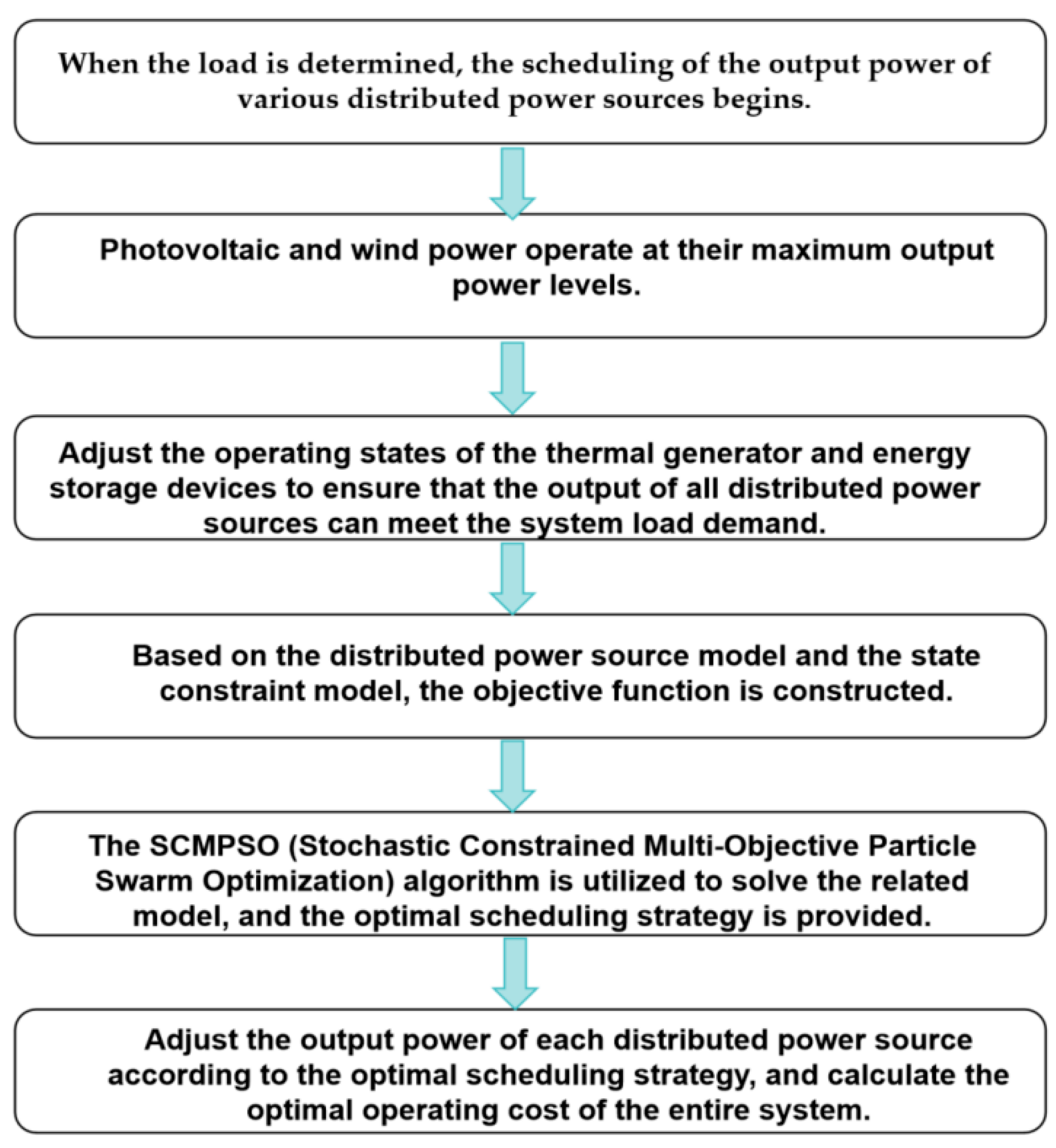
3.3. Scheduling Strategy

The microgrid consists of numerous distributed power sources, some of which generate electricity using clean energy. These new types of distributed power sources have different characteristics compared to traditional generators in conventional power grids:

• PV and WT: PV generation relies on solar energy, while wind-power generation depends on wind energy. Both are clean energy sources. Although they exhibit significant fluctuations, fully utilizing these resources helps reduce generation costs and avoids environmental pollution.
• Thermal Power Generation: Currently, thermal power remains an indispensable part of China’s power system. Its advantage lies in providing stable electricity that is capable of meeting large load demands. However, the downside of thermal power generation is the significant consumption of fossil fuels and its associated environmental pollution.
• Energy Storage Devices: Energy storage systems have the advantage of fast response times. In microgrid systems, they effectively buffer the impact of PV and wind-power integration on the main grid, ensuring stable system operation.

Based on these characteristics, the following scheduling strategy is proposed: To ensure stable operation of the microgrid, priority is given to fully utilizing PV and wind-power generation. Due to the variability of PV and wind power, energy storage devices are used to adjust and buffer the system. On this foundation, thermal generators are employed to supplement the power supply as needed, thereby guaranteeing the system’s stable and continuous operation.

Figure 1 represents the flowchart of the optimized scheduling process.

4. Improved Second-Order Oscillation Particle Swarm Optimization Algorithm

4.1. Traditional Particle Swarm Optimization

The Particle Swarm Optimization (PSO) technique is inspired by the collective movement of birds and operates as a stochastic optimization strategy based on group behavior. Within this framework, each particle represents a possible solution [23]. The strength of the PSO lies in its iterative process, where the group continuously compares fitness values and adjusts the best positions, eventually leading to both the individual and global optimal solutions. The velocity and position update formulas for the particles in the PSO are as follows:

$$V_i^{k+1}=w{\mathrm{V}}_i^k+r_1{c}_1(X{pbest}_i^k-x_i^k)+r_2{c}_2({Xgbest}_i^k-x_i^k)$$

(23)

$$X_i^{k+1}=X_i^k+V_i^{k+1}$$

(24)

In these equations, $w$ is the inertia weight, representing the particle’s search speed; $c_1$ is the individual learning factor, which controls the particle’s movement toward its best position; $c_2$ is the group learning factor, controlling the movement of all particles toward the global best position; r₁ and r₂ are random numbers in the range [0, 1]; ${\mathrm{V}}_i^k$ is the current particle’s velocity, $X{pbest}_i^k$ is the current individual’s best position, and ${Xgbest}_i^k$ is the global best position in the k-th iteration.

However, traditional PSO frequently encounters local optima, suffers from early convergence, and leads to an uneven distribution of particles within the search space throughout the iterative process. To avoid these shortcomings, we propose improvements to the PSO algorithm.

4.2. Chaotic Mapping Second-Order Oscillation Particle Swarm Optimization

4.2.1. Chaotic Mapping Population

In traditional PSO, the randomly generated initial population positions and particle velocities often lead to an uneven spatial distribution of particles in the early stages of the iterative search. This uneven initial distribution significantly affects the global search capability of the algorithm. To prevent the initial particle population from falling into local search traps, we introduce chaotic mapping during the population initialization phase to initialize the particle positions [24,25]. By adopting chaotic mapping to initialize the particle positions, we can expand the global search range and increase the randomness of the particles. In this study, Henon mapping is used to generate random numbers as the initial positions of the population, thereby enhancing particle diversity and significantly speeding up the algorithm’s global convergence, improving its overall performance.

The Henon mapping expression for population initialization is as follows:

$${\mathrm{X}}_{\mathrm{i}+1}^{\mathrm{k}}=\mathrm{F}(\mathrm{x},\mathrm{r})=1-\mathrm{a}\times {\mathrm{X}}_{\mathrm{i}}^{\mathrm{k}}^2+\mathrm{b}\times {\mathrm{X}}_{\mathrm{i}}^{\mathrm{k}}$$

(25)

In this equation, a and b are control parameters, also known as chaotic mapping parameters. The parameter a primarily influences the population’s nonlinearity; higher values of a increase the chaotic nature of the population. The parameter b controls the system’s symmetry and coupling strength, affecting the overall trajectory of the population, with smaller values usually used for b. The value range for a is [1, 2], and for b, it is [0, 1].

The steps for initializing the population using Henon mapping are as follows:

• Define the chaotic Henon mapping function to produce a D-dimensional vector, where each value within the vector is confined to the range of rand(0.1).
• Map the population positions using the chaotic Henon function.

4.2.2. Adaptive Weight Iteration Improvement

In PSO, global search mainly occurs in the early stages of the algorithm. When the inertia weight w is large, it may lead to an excessive global search, slowing down convergence and causing oscillations and instability in the population. On the other hand, if w is small, it can result in an excessive local search, making the algorithm prone to falling into local optima and failing to maintain population diversity.

To balance the global and local searches, we use an adaptive inertia weight iteration method. As the population iterates, the inertia weight is dynamically adjusted based on the situation [26]. In the early iterations, a greater inertia weight is assigned to improve the ability for global search; subsequently, this weight is systematically decreased in a non-linear fashion to strengthen local search ability. The inertia weight expression is as follows:

$$\mathrm{b}={\displaystyle \frac{{\mathrm{f}\mathrm{i}\mathrm{t}}_{\mathrm{i}}-{\mathrm{f}\mathrm{i}\mathrm{t}}_{\mathrm{g}\mathrm{b}\mathrm{e}\mathrm{s}\mathrm{t}}}{{\mathrm{f}\mathrm{i}\mathrm{t}}_0-{\mathrm{f}\mathrm{i}\mathrm{t}}_{\mathrm{g}\mathrm{b}\mathrm{e}\mathrm{s}\mathrm{t}}}}$$

(26)

$$\mathrm{w}=\left\{\begin{array}{c}{\mathrm{w}}_{\mathrm{m}\mathrm{a}\mathrm{x}}+({\mathrm{w}}_{\mathrm{m}\mathrm{a}\mathrm{x}}-{\mathrm{w}}_{\mathrm{m}\mathrm{i}\mathrm{n}})(1-{\displaystyle \frac{1}{\mathrm{b}}}),b\ge 1\\ {\mathrm{w}}_{\mathrm{m}\mathrm{i}\mathrm{n}}+b({\mathrm{w}}_{\mathrm{m}\mathrm{a}\mathrm{x}}-{\mathrm{w}}_{\mathrm{m}\mathrm{i}\mathrm{n}}),b<1\end{array}\right.$$

(27)

In Equation (26), fit_i represents the fitness of the current particle, fit_gbest represents the best fitness in the population, and fit₀ represents the critical fitness of the population. In Equation (27), w_max is the maximum weight factor, set to 0.9, and w_min is the minimum weight factor, set to 0.4.

4.2.3. Dynamic Learning Factor Improvement

In the early iterations of the algorithm, emphasis must be placed on global search abilities to guarantee diversity within the population. During the middle and advanced phases of the algorithmic process, more attention should be given to local search capabilities and algorithm convergence. Therefore, the learning factors $c_1$ and $c_2$ in the algorithm need to be dynamically adjusted as the iteration progresses. To enhance the reliability of the algorithm, $c_1$ is set as a monotonically decreasing function, while c₂ is set as a monotonically increasing function. The specific expressions are as follows:

$$c_1=2\times {sin}^2\left[{\displaystyle \frac{\pi }{2}}\right(1-{\displaystyle \frac{t}{Tmax}}\left)\right]$$

(28)

$$c_2=2\times {sin}^2\left({\displaystyle \frac{\pi t}{2Tmax}}\right)$$

(29)

In Equations (28) and (29), $t$ represents the current iteration number, and $Tmax$ represents the maximum number of iterations. By continuously adjusting the learning factors during the iteration process, this approach can accelerate the speed at which the population finds the optimal solution. Figure 2 is a trend graph of the learning factor iteration for 2000.

4.2.4. Improvement in Algorithm Iteration

In the PSO, the update of a particle’s velocity is mainly influenced by its own best-known position and the best position discovered by the entire swarm. However, the relative position of a single particle is not fully considered in the PSO. To improve the accuracy of the global search and reduce the convergence time, this paper introduces an oscillation variable. During the iteration process, perturbations are introduced near the optimal solution to bolster the diversity among the population’s solutions, thus minimizing the risk of the algorithm getting trapped in local minima. The iteration formula is as follows:

$$V_i^{k+1}=w{v}_i^k+u_1[X{pbest}_i^k-(1+{\lambda }_1)X{gbest}_i^k+{\lambda }_{1}X{gbest}_i^{k-1}]+u_2[X{pbest}_i^k-(1+{\lambda }_2)X{gbest}_i^k+{\lambda }_{2}X{gbest}_i^{k-1}]$$

(30)

In Equation (30), ${\lambda }_1$ and ${\lambda }_2$ are the factors for progressive convergence and oscillation convergence of the particle swarm.

$$u_1=c_1\ast r_1, c_1=2\ast {sin}^2\left[{\displaystyle \frac{\pi }{2}}\right(1-{\displaystyle \frac{t}{Tmax}}\left)\right] ,r_1=random$$

(31)

$$u_2=c_2\ast r_2, c_2=2\ast {sin}^2\left({\displaystyle \frac{\pi t}{2Tmax}}\right) ,r_2=random$$

(32)

When the iteration count t ≤ $Tmax$/2, the algorithm exhibits oscillation convergence:

$${\lambda }_1\ge {\displaystyle \frac{2\sqrt{c_1{r}_1}-1}{c_1{r}_1}} {\lambda }_2\ge {\displaystyle \frac{2\sqrt{c_2{r}_2}-1}{c_2{r}_2}}$$

(33)

When the iteration count t > $Tmax$/2, the algorithm exhibits progressive convergence:

$${\lambda }_1\le {\displaystyle \frac{2\sqrt{c_1{r}_1}-1}{c_1{r}_1}} {\lambda }_2\le {\displaystyle \frac{2\sqrt{c_2{r}_2}-1}{c_2{r}_2}}$$

(34)

Figure 3 is a trend graph of the oscillation curve. Figure 4 is a trend graph of the progressive curve, with specific trends as follows.

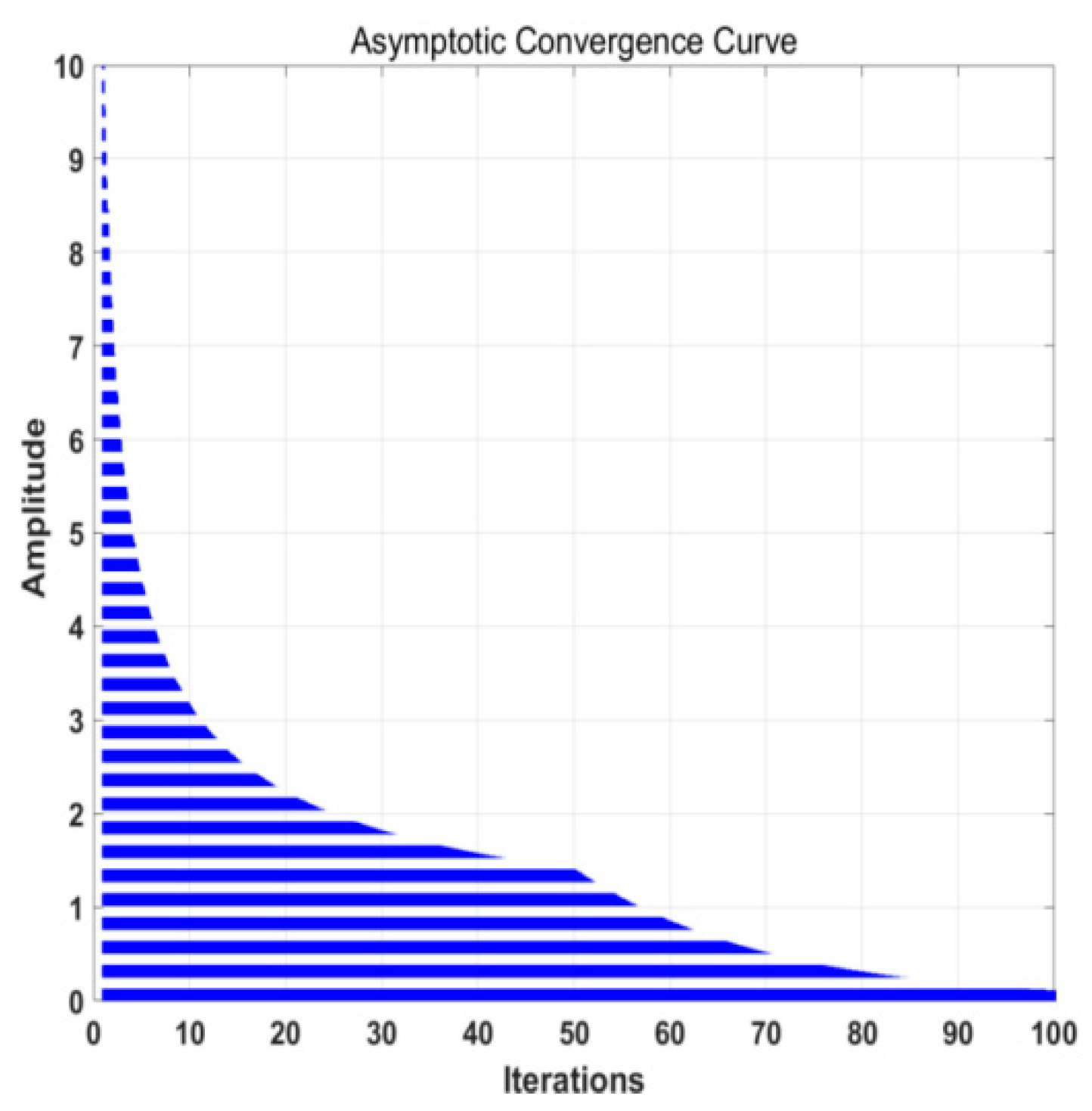
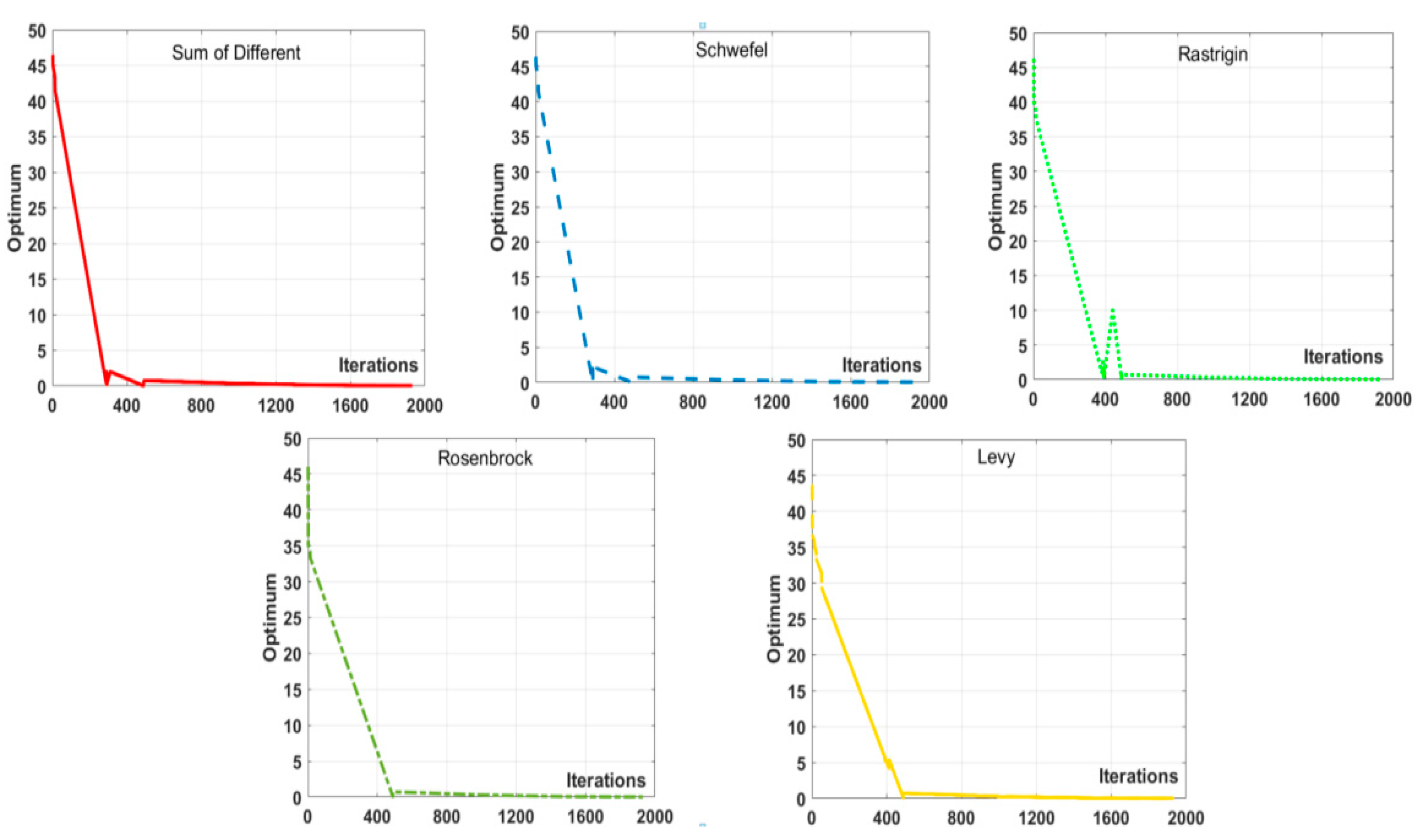
4.2.5. Testing of the Improved Particle Swarm Algorithm

To assess the effectiveness of the enhanced PSO algorithm, a selection of benchmark functions was utilized for testing. These benchmark functions comprise the following five elements:

• Sum of Different Powers: This function serves as a tool to evaluate the convergence rate of the enhanced algorithm;
• Schwefel: Used to test the precision of the search conducted by the improved algorithm;
• Rastrigin: Used to test the algorithm’s ability to avoid getting stuck in local minima;
• Rosenbrock: Used to evaluate the performance of the improved algorithm in a multi-dimensional space;
• Levy: Used to test the robustness of the algorithm. The relevant parameters for the benchmark functions are shown in

  Table 3. Relevant parameters of benchmark functions.

  Function Name	Dimension	Search Domain	Acceptance	Optimum
  Sum of Different Powers	50	[−10,10]D [−100,100]n[−100,100]n [−100,100]n[−100,100]n	0.01	0
  Schwefel	50	[−100,100]D	0.01	0
  Rastrigin	50	[−5,5]D	0.01	0
  Rosenbrock	50	[−50,5]D	0.01	0
  Levy	50	[−10,10]D	0.01	0

  .

To verify the advantages of the SCMPSO algorithm in terms of convergence and accuracy compared to the original PSO and other improved algorithms, we conducted comparative experiments under the same parameter settings between the second-order oscillating PSO and other algorithms. The basic experimental conditions were as follows: population size of 100, dimension of 50, and 2000 iterations. The test results of the benchmark functions are shown in Figure 5, and the comparison results between the improved second-order oscillating PSO and other algorithms are shown in Figure 6.

Figure 5 shows the test results of the SCMPSO algorithm using five benchmark functions. The results indicate that the SCMPSO algorithm demonstrates certain advantages in convergence speed, global search range, search accuracy, and escaping local optima. Figure 6 compares the SCMPSO algorithm with several other PSO algorithms. It can be seen that when the population iterates to around 500 times, the results of the four PSO algorithms tend to approach 0. To guarantee the reliability of the algorithm, it is crucial that the number of iterations does not fall below 500. To avoid insufficient validation of the algorithm’s effectiveness due to too few iterations, 2000 iterations were chosen as the standard in this paper.

4.3. Model Solution

The improved SCMPSO algorithm can be applied to solve the optimization problem presented in this paper. The detailed steps of the algorithm are shown in Figure 7:

Step 1: Initialize the basic parameters of the SCMPSO algorithm, which include 100 particles, 50 dimensions per particle, and 2000 iterations. Set the initial iteration to 0 and define the scheduling period as 24 h.

Step 2: Input the load data, electricity price data, and parameters for photovoltaic systems, wind generation systems, thermal generators, and energy storage devices.

Step 3: Initialize the particle population and assign values to the dimensions.

Step 4: Based on the scheduling strategy and constraints, adjust the operating states of the photovoltaic systems, wind generators, thermal generators, and energy storage units.

Step 5: Check whether the maximum iteration limit has been reached. If so, output the current scheduling strategy, the optimal particle fitness value, and the system’s minimum operating cost.

Step 6: If the iteration limit has not yet been reached, continue by updating the positions and velocities of the particles and the global best position of the population. Then, calculate the current individual and global best fitness values.

Step 7: Revise the scheduling strategy based on the individual and global best positions and their corresponding optimal fitness values, and calculate the system’s current minimum operating cost.

Step 8: Check again whether the maximum iteration count has been reached. If reached, output the required results; otherwise, repeat Steps 6 and 7.

5. Case Study

This study conducts a case analysis based on typical summer environmental data from a city in Jiangsu Province, China. Using the improved SCMPSO algorithm combined with a scheduling strategy, interaction parameters between distributed generation, microgrids, and the main grid were obtained. In this paper, the improved SCMPSO algorithm is applied to case simulations for optimization, and the relevant parameters after optimization are provided.

5.1. Case Introduction

The multi-source microgrid system structure used in this study is shown in Figure 8. The microgrid system includes 10 distributed photovoltaic generation units (each with a rated power of 10 kW), wind-power generation equipment (rated power of 10 kW), a thermal generator (rated power of 1000 kW), and 2 energy storage units (each with a rated power of 10 kW). In the case analysis, both residential and industrial electricity consumption were considered. The scheduling period is 24 h, with a time interval of 1 h.

The data pertinent to the case study are shown in Figure 9, Figure 10 and Figure 11. Figure 9 presents typical daily load data for the summer season. Jiangsu Province, China, has a subtropical monsoon climate characterized by hot and rainy summers. Figure 10 shows the typical wind speed in summer, Figure 11 illustrates the typical temperature conditions during summer, and Figure 12 provides the solar irradiance data.

Table 4. Microgrid system power purchase and sale price.

Time Period	Peak Period 11:00–14:00, 19:00–21:00	Standard Period 8:00–10:00, 15:00–18:00, 22:00–23:00	Off-Peak Period 0:00–7:00
Electricity Purchase Price (RMB/kWh)	0.83	0.49	0.17
Electricity Sale Price (RMB/kWh)	0.65	0.38	0.13

lists the electricity purchase and sale prices for the microgrid system at different periods.

5.2. Simulation Analysis

Based on the scheduling strategy proposed in Section 3.3, the output power of PV and wind-power generation equipment is maximized under the premise of meeting load demand. Based on this, the generator’s output power is progressively decreased to minimize the overall operational expenses of the system. Since the selected time period is in the summer, with high solar irradiance, the energy storage device can store electricity during periods of high solar intensity and release it when solar intensity decreases, reducing system fluctuations. Based on the scheduling strategy, the SCMPSO algorithm is used for simulation analysis. The simulation provides the output power of each distributed energy source during a typical summer day, as well as the microgrid’s electricity purchase and sale situation. Figure 13 illustrates the output power curves of the distributed energy sources over 24 h.

In summer, compared to other seasons, the increase in load is primarily concentrated on cooling and air conditioning. With the goal of meeting the load demand, clean energy sources such as PV and wind power should be fully utilized while energy storage devices are used to regulate the system’s stability. When small thermal generators, PV, wind power, and energy storage devices cannot meet the power demand, purchasing electricity from the main grid is considered to compensate for the power shortage.

Figure 14 illustrates the electricity transaction scenario of the microgrid system, which fully leverages PV, wind, and energy storage devices for both purchasing and selling purposes. In the figure, the electricity purchase is represented below the horizontal axis, indicating power bought from the main grid, while the electricity sale is shown above the axis, indicating power sold to the main grid. This figure clearly illustrates the microgrid system’s electricity trading status at different times, helping to evaluate the economic operation of the system.

• Electricity Purchase Period (00:00–04:00, 22:00–24:00)

During the periods from 00:00 to 04:00 and from 22:00 to 24:00, as shown in Figure 13 and Figure 14, neither the photovoltaic (PV) nor the wind-power generation equipment outputs power, while the energy storage device releases energy. However, the output power of the small thermal generator is still insufficient to cover the microgrid’s load demand. As a result, the microgrid needs to purchase electricity from the main grid to fulfill its energy requirements.

2.

No Interaction Period between Microgrid and Main Grid (05:00–09:00, 16:00–21:00)

During the periods from 05:00 to 09:00 and from 16:00 to 21:00, as shown in Figure 13 and Figure 14, the output power of the distributed energy sources within the microgrid (such as PV and similar systems) is balanced with the microgrid’s load demand. During this time, the microgrid is self-sufficient, requiring no electricity interaction with the main grid, meaning that no electricity is purchased or sold.

3.

Electricity Sale Period (10:00–15:00)

During the period from 10:00 to 15:00, as shown in Figure 13 and Figure 14, the output power generated by the distributed energy sources within the microgrid, including PV and wind-power equipment, surpasses the load demand of the microgrid. In this case, the microgrid has the capability to sell the excess electricity to the main grid, thereby optimizing its economic returns.

Table 5. Output power of distributed energy sources and their interaction power with the main grid.

Time Period	System Load Power/kW	PV/kW	WT/kW	DG/kW	ESS/kW	Interactive Power/kW
00:00–01:00	510.34	0	1.32	425.98	45.81	38.55
01:00–02:00	480.52	0	0	420.98	444.98	14.56
02:00–03:00	440.91	0	0	400	38.18	2.73
03:00–04:00	430.16	0	0	400	29.95	1.21
04:00–05:00	380.59	0	0	380.59	0	0
05:00–06:00	385.37	70.12	1.27	313.98	0	0
06:00–07:00	400.64	71.36	1.43	327.85	0	0
07:00–08:00	410.69	73.59	1.75	337.3	−1.95	0
08:00–09:00	450.73	78.65	2.15	410.69	−40.76	0
09:00–10:00	650.12	82.13	4.27	500.32	−150.73	−214.13
10:00–11:00	680.49	83.32	2.21	510.3	−130.98	−215.64
11:00–12:00	720.95	87.95	1.95	520.67	−157.73	−268.11
12:00–13:00	700.76	90.12	1.93	520.4	−180.85	−269.16
13:00–14:00	650.48	91.32	1.89	530.64	−193.13	−219.76
14:00–15:00	630.39	93.28	1.83	547.6	−170.46	−158.14
15:00–16:00	600.75	91.7	1.77	547.6	−40.68	0
16:00–17:00	580.13	90.12	1.74	528.95	−40.68	0
17:00–18:00	570.48	85.69	1.83	526.91	−43.95	0
18:00–19:00	550.72	79.48	1.77	427.52	41.95	0
19:00–20:00	570.09	77.95	1.74	450.22	40.18	0
20:00–21:00	600.48	0	1.27	555.26	43.95	0
21:00–22:00	610.87	0	0	550.79	47.68	12.4
22:00–23:00	615.48	0	0	540.39	445.48	29.61
23:00–24:00	580.48	0	0	480.37	47.35	52.76

visually presents the output power of various distributed energy sources and their interaction with the main grid. This table provides insight into the energy exchange status between the distributed energy sources, the microgrid, and the main grid system during different time periods, offering a basis for the subsequent scheduling plan.

Table 6. Economic cost of system operation.

Types	Types of Costs	Operation and Maintenance Cost/RMB	Fuel Cost/RMB	Depreciation Cost/RMB	Grid Interaction Cost/RMB	Environmental Cost/RMB
SCMPSO	detailed data	3542.64	2865.43	712.86	−642.80	95.17
CPSO	detailed data	3615.72	2931.54	722.65	−554.18	100.59
QPSO	detailed data	3684.42	2955.17	740.43	−541.75	103.05
PSO	detailed data	3773.59	3170.43	757.29	−500.48	108.72

shows the daily economic costs of the system optimized by the SCMPSO, CPSO, QPSO, and PSO algorithms.

Table 6 presents the economic costs of the system under optimization by four different algorithms. As shown in the figure, the SCMPSO algorithm demonstrates significant advantages in terms of system operating costs, fuel costs, and environmental management costs. With the current global emphasis on environmental protection and carbon emission reduction, the SCMPSO algorithm stands out with the lowest environmental management costs and the lowest pollutant emissions, aligning well with these global objectives.

Table 7. Pollutant emissions and treatment costs under four optimization algorithms.

Types	CO2 Emissions (KG)	CO2 Treatment Cost/RMB	SO2 Emissions (KG)	SO2 Treatment Cost/RMB	NOX Emissions (KG)	NOX Treatment Cost/RMB	Environmental Cost/RMB
SCMPSO	224.765	44.953	0.17	2.465	0.752	47.752	95.17
CPSO	247.675	49.535	0.184	2.668	0.762	48.387	100.59
QPSO	256.0925	51.2185	0.185	2.6825	0.774	49.149	103.05
PSO	278.075	55.615	0.194	2.813	0.792	50.292	108.72

presents the pollutant emissions and their treatment costs under four different optimization algorithms. It is clear from the table that, after optimization by the SCMPSO algorithm, both the microgrid and main grid systems exhibit significantly lower pollutant emissions, thereby minimizing environmental pressure. Furthermore, the SCMPSO algorithm not only reduces pollutant emissions but also effectively controls treatment costs, achieving a better balance between economic benefits and environmental protection. These optimization results highlight the potential of the SCMPSO algorithm in promoting sustainable development.

6. Conclusions

Based on the operating characteristics of various distributed energy sources in the microgrid system, this study established an optimization model and, with the goal of ensuring a stable system operation, used SCMPSO for simulation and optimization. The following conclusions were drawn:

• Typical Summer Dispatch Plan: In a subtropical monsoon climate, such as in a certain region of Jiangsu, China, summer is characterized by heat and abundant sunlight. Based on the scheduling strategy and comprehensive cost considerations, the specific dispatch plan is as follows: distributed photovoltaic (PV) and wind-power generation should be fully utilized as much as possible. On this basis, to ensure a stable system operation, small thermal generators must bear the main power output. Additionally, energy storage devices play a key role in peak shaving and valley filling, as well as improving power quality. This dispatch plan not only guarantees system stability but also increases the utilization of clean energy, reduces environmental pollution, and enhances overall economic efficiency.
• SCMPSO: Compared to the traditional PSO algorithm, the SCMPSO algorithm accelerates the search speed and broadens the search range in the early stages of optimization, while effectively avoiding local optima in the later stages. The reliability and superiority of the SCMPSO algorithm were confirmed through validation with multiple benchmark functions.

References

1. Yao, Y.; Du, H.; Zou, H.; Zhou, P.; Antunes, C.H.; Neumann, A.; Yeh, S. Fifty years of Energy Policy: A bibliometric overview. Energy Policy 2023, 183, 113769. [Google Scholar] [CrossRef]
2. Feng, C.; Liao, X. An overview of “Energy þ Internet” in China. J. Clean. Prod. 2020, 258, 120630. [Google Scholar] [CrossRef]
3. Duan, Y.; Zhao, Y.; Hua, J. An initialization-free distributed algorithm for dynamic economic dispatch problemsinmicrogrid: Modeling, optimization and analysis. Sustain. Energy Grids Netw. 2023, 34, 101004. [Google Scholar] [CrossRef]
4. Abdelghany, M.B.; Al-Durra, A.; Gao, F. A Coordinated Optimal Operation of a Grid-Connected Wind-Solar Microgrid Incorporating Hybrid Energy Storage Management Systems. IEEE Trans. Sustain. Energy 2024, 15, 39–51. [Google Scholar] [CrossRef]
5. Gholami, A.; Shekari, T.; Aminifar, F.; Shahidehpour, M. Microgrid scheduling with uncertainty: The quest for resilience. IEEE Trans. Smart Grid 2016, 7, 2849–2858. [Google Scholar] [CrossRef]
6. Correa-Posada, C.M.; Sánchez-Martın, P. Security-constrained optimal power and natural-gas flow. IEEE Trans. Power Syst. 2014, 29, 18–24. [Google Scholar] [CrossRef]
7. Sadeghian, H.; Ardehali, M. A novel approach for optimal economic dispatch scheduling of integrated combined heat and power systems for maximum economic profit and minimum environmental emissions based on Benders decomposition. Energy 2016, 102, 10–23. [Google Scholar] [CrossRef]
8. Shen, X.; Cao, M.; Zhou, N.; Zhang, L. Research on coordinated optimal scheduling and economic operation of multi-microgrid distribution system. J. Electron. Meas. Instrum. 2016, 30, 568–576. [Google Scholar]
9. Yin, L.; Cai, Z. Multimodal multi-objective hierarchical distributed consensus method for multimodal multi-objective economic dispatch of hierarchical distributed power systems. Energy 2024, 295, 130996. [Google Scholar] [CrossRef]
10. Rezaei, N.; Ahmadi, A.; Khazali, A.; Aghaei, J. Multi-objective risk-constrained optimal bidding strategy of smart microgrids: An IGDT-based normal boundary intersection approach. IEEE Trans. Ind. Inf. 2018, 15, 1532–1543. [Google Scholar] [CrossRef]
11. Huang, Z.; Xu, L.; Wangb, B.; Li, J. Optimizing power systems and microgrids: A novel multi-objective model for energy hubs with innovative algorithmic optimization. Int. J. Hydrogen Energy 2024, 69, 927–943. [Google Scholar] [CrossRef]
12. Zhao, F.; Ji, F.; Xu, T.; Zhu, N.; Jonrinaldi. Hierarchical parallel search with automatic parameter configuration for particle swarm optimization. Appl. Soft Comput. J. 2024, 151, 111126. [Google Scholar] [CrossRef]
13. Wang, C. The Optimal Operation of Microgrid Based on Improved Particle Swarm Optimization for Combined Cooling, Heating and Power. Master’s Thesis, China University of Mining and Technology, Beijing, China, 2022. [Google Scholar]
14. Xiong, G.J.; Shuai, M.H.; Hu, X. Combined heat and power economic emission dispatch using improved bare bone multi-objective particle swarm optimization. Energy 2022, 244, 123108. [Google Scholar] [CrossRef]
15. Jakubik, J.; Binding, A.; Feuerriegel, S. Directed particle swarm optimization with Gaussian-process-based function forecasting. Eur. J. Oper. Res. 2021, 295, 157–169. [Google Scholar] [CrossRef]
16. Zhao, X.G.; Zhang, Z.Q.; Xie, Y.M.; Meng, J. Economic-environmental dispatch of microgrid based on improved quantum particle swarm optimization. Energy 2020, 195, 117014. [Google Scholar]
17. Kacimi, M.A.; Guenounou, O.; Brikh, L.; Yahiaoui, F.; Hadid, N. New mixed-coding PSO algorithm for a self-adaptive and automatic cleaning of Mamdani fuzzy rules. Eng. Appl. Artif. Intell. 2020, 89, 103417. [Google Scholar] [CrossRef]
18. Wang, Y.; Zhang, H.; Zhang, G. CPSO-CNN: An efficient PSO-based algorithm for fine-tuning hyper-parameters of convolutional neural networks. Swarm Evol. Comput. 2019, 49, 114–123. [Google Scholar] [CrossRef]
19. Roudbari, F.N.; Ehsani, H.; Amiri, S.R.; Samadani, A.; Shabani, S.; Khodadad, A. Advances in photovoltaic thermal systems: A comprehensive review of CPVT andPVT technologies. Sol. Energy Mater. Sol. Cells 2024, 276, 113070. [Google Scholar] [CrossRef]
20. Teferra, D.M.; Ngoo, L.M.; Nyakoe, G.N. Fuzzy-based prediction of solar PV and wind power generation for microgrid modeling using particle swarm optimization. Heliyon 2023, 9, e12802. [Google Scholar] [CrossRef]
21. Ding, M.; Wang, B.; Zhao, B.; Chen, Z.N. Configuration optimization of capacity of standalone PV-wind-diesel battery hybrid microgrid. Power Syst. Technol. 2013, 37, 575–581. [Google Scholar]
22. Zhang, J.; Su, L.; Chen, Y.; Su, J.; Wnag, L. Energy management of microgrid and its control strategy. Power Syst. Technol. 2011, 35, 24–28. [Google Scholar]
23. Liu, J.; Xu, F.; Lin, S.; Cai, H.; Yan, S. A multi-agent-based optimization model for microgrid operation using dynamic guiding chaotic search particle swarm optimization. Energies 2018, 11, 3286. [Google Scholar] [CrossRef]
24. Chu, S.-C.; Panb, X.Y.J.-S.; Lin, B.-S.; Lee, Z.-J. Amulti-strategy surrogate-assisted social learning particle swarm optimization for expensive optimization andapplications. Appl. Soft Comput. J. 2024, 162, 11187. [Google Scholar] [CrossRef]
25. Priya, G.V.; Ganguly, S. Multi-swarm surrogate model assisted PSO algorithm to minimize distribution network energy losses. Appl. Soft Comput. J. 2024, 159, 111616. [Google Scholar] [CrossRef]
26. Tantu, A.T.; Biramo, D.B. Power flow control and reliability improvement through adaptive PSO based network reconfiguration. Heliyon 2024, 10, e36668. [Google Scholar] [CrossRef]
Figure 1. Optimized scheduling flowchart.
Electronics 13 04086 g001
Figure 2. Learning factor iteration graph.
Electronics 13 04086 g002
Figure 3. Oscillation convergence curve.
Electronics 13 04086 g003
Figure 4. Progressive convergence curve.
Electronics 13 04086 g004
Figure 5. Test results of each benchmark function.
Electronics 13 04086 g005
Figure 6. Iteration comparison of different Particle Swarm Optimization algorithms.
Electronics 13 04086 g006
Figure 7. Algorithm Flowchart.
Electronics 13 04086 g007
Figure 8. Multi-source microgrid structure.
Electronics 13 04086 g008
Figure 9. Daily load data diagram.
Electronics 13 04086 g009
Figure 10. Typical summer wind speed.
Electronics 13 04086 g010
Figure 11. Typical summer 24-h temperature.
Electronics 13 04086 g011
Figure 12. Measurement of 24-h solar irradiance intensity.
Electronics 13 04086 g012
Figure 13. Image of 24-h power curves of distributed energy sources and energy storage devices.
Electronics 13 04086 g013
Figure 14. Diagram of electricity purchase and sale between microgrid and main grid system.
Electronics 13 04086 g014