Station-Keeping Control of Stratospheric Balloons Based on Simultaneous Optimistic Optimization in Dynamic Wind

Abstract

Stratospheric balloons serve as cost-effective platforms for wireless communication. However, these platforms encounter challenges stemming from their underactuation in the horizontal plane. Consequently, controllers must continually identify favorable wind conditions to optimize station-keeping performance while managing energy consumption. This study presents a receding horizon controller based on wind and balloon models. Two neural networks, PredRNN and ResNet, are utilized for short-term wind field forecast. Additionally, an online receding horizon controller, based on simultaneous optimistic optimization (SOO), is developed for action sequence planning and adapted to accommodate various constraints, which is especially suitable due to its gradient-free nature, high efficiency, and effectiveness in black-box function optimization. A reward function is formulated to balance power consumption and station-keeping performance. Simulations conducted across diverse positions and dates demonstrate the superior performance of the proposed method compared with traditional greedy and A* algorithms.

1. Introduction

Stratospheric balloons, as a type of high-altitude platform (HAP), have great potential to provide wireless communication for satellites, terrestrial systems, and offshore users, offering low signal delays and high resilience for months. Although their channel capacity is lower compared with terrestrial stations, HAPs can service areas ranging from 60 km to 400 km in diameter [1,2]. Moreover, HAPs exhibit superior propagation performance and higher signal-to-noise ratios compared with that of low earth orbit satellites, making them an essential option for wireless communication especially for rural areas.

Novel stratospheric balloons, as lighter-than-air vehicles, can control their working altitude between 18 and 22 km by pumping air in or out. Additionally, their horizontal movement is dominated by the local winds. Therefore, balloon controllers should be able to continuously seek favorable wind layers over extended periods during station-keeping missions. Further, energy balance and restricted flight zone should also be taken into consideration. To maintain the balloon above a fixed ground station, an indirect trajectory should be taken through the wind field.

1.1. Balloon Control

In Project Loon, Bellmare [3] compared a rule-based method, optimistic deterministic planning (OPD), and reinforcement learning (RL) for station-keeping navigation. It was found that RL leveraged wind field information and past flight data, yielding results with superior computational efficiency. Sniderman [4] investigated formation control of large balloon fleets along specified latitudes. A distributed control method was proposed that each balloon adjusted its position relative to the next one to minimize errors in virtual formation placement; it achieved consensus when longitudinal distances were equal. Vandermeulen [5] employed distributed extremum-seeking control (ESC), a data-driven approach, for formation control. Parameters such as balloon distance, coverage area, internet bandwidth, and connected users were considered in the loss function. ESC continuously explored and exploited the action space to enhance network performance. Rossi [6] studied autonomous navigation and exploration of Venusian volcanism. Dynamic programming with stochastic wind flow models was employed, which increased close-up observations of volcanic events by 63% compared with passive drifters, demonstrating robustness in uncertain flow conditions.

1.2. Wind Speed Forecast

Wind speed forecast is critical for balloon station- keeping. Traditional methods of weather forecast rely on two primary approaches: numerical weather prediction (NWP) and statistical methods. NWP incorporates complex physical models and data assimilation, which updates every 6 to 12 h. In contrast, statistical methods are more effective for short-term predictions (less than 6 h) [7]. Recently, neural network-based approaches have been developed rapidly and offer comparable accuracy with high efficiency. These techniques have been successfully employed in medium-range global forecasts [8,9,10], nowcasting [11,12,13], and wind power prediction [14,15].

For medium-range global forecasts, Kochkov [10] integrated physical processes, such as aerodynamics and thermodynamics, with neural networks to forecast wind speed and predict unresolved processes, including precipitation, humidity, and cloud formation. This approach is computationally efficient, exhibits low complexity, and yields more interpretable results. For precipitation nowcasting, Ravuri [12] developed a recurrent neural network utilizing convolutional gated recurrent units. This network extracts temporal features to predict 18 future precipitation fields over a 90-min period. The method has demonstrated superior capabilities in predicting spatial coverage and convection over extended periods without overestimating intensities. Zhang [13] proposed a two-path U-Net to model both the motion and intensity of precipitation, utilizing motion regularization and accumulation loss to enhance accuracy in predicting both position and intensity. For wind power prediction, Acikgoz [14] applied variational mode decomposition as a preprocessing step and implemented a convolutional neural network (CNN) with a channel attention module to forecast wind speed for wind farms, achieving competitive performance.

The application of neural networks to forecasting tasks represents a significant advancement in predicting wind speed and related weather phenomena. These methods leverage rich historical data to produce increasingly accurate and reliable forecasts across various meteorological domains.

1.3. Optimistic Optimization

Optimistic optimization is a numerical, gradient-free optimization method for black-box functions, with the key assumption that the function is Lipschitz continuous. The technique approximates unknown functions using upper bounds, guiding the selection of sample points for expansion. Thus, the guiding principle behind this class of strategies is to be optimistic in the face of uncertainty [16]. A well-known application of this concept is the K-armed bandit problem, where the upper confidence bound principle is used [17]. In Bayesian optimization, this principle helps balance exploration and exploitation, leading to exponentially vanishing instantaneous regret [16].

Wang [18] introduced BaSOO, which combined Bayesian optimization with simultaneous optimistic optimization (SOO). This method used Gaussian processes (GP) to estimate unknown sample points, reducing iterations. However, BaSOO is slower than SOO due to the GP’s additional expansion and rejection of sample points, so it is more suited for functions with high computational demands. Busoniu [19] applied optimistic optimization to continuous planning problems, demonstrating its effectiveness.

While RL and dynamic programming offer global solutions, they are often constrained by the dimensionality of the state space [17]. ESC struggles with non-convex problems and balancing exploration with exploitation in dynamic wind conditions. Traditional hierarchical trajectory planning methods are inadequate for under-actuated systems and discrete action spaces. This paper adopts the SOO-based planning (SOOP) method proposed in [17], modified for constraints. SOOP proves highly efficient for discrete action spaces and model-driven planning.

The main contributions are as follows:

• Two neural networks, based on a residual convolutional network and a recurrent neural network, are proposed for wind forecast. They are more accurate than a persistence model.
• A receding horizon control approach, based on SOOP, is proposed for the station-keeping problem under multiple constraints. This method outperforms both the greedy approach and A*.
• This is the first work to combine deep wind forecasting with planning techniques for balloon control. The solution is both efficient and asymptotically optimal.

2. Deep Learning for Wind Speed Forecast

Two networks are developed for wind speed forecast. The first one is a recurrent neural network; it has minimal forecast error in 1–3 h, and the error accumulates rapidly. Additionally, the second one is a residual convolutional neural network. It has minimal forecast error in 4 h.

2.1. PredRNN

PredRNN [20] is a recurrent neural network (RNN) designed for spatiotemporal predictive learning. It benefits many practical applications, such as traffic flow prediction [21] and video frame prediction. PredRNN is highly suited for tasks requiring simultaneous modeling of spatial and temporal information. Its architecture consists of stacked convolutional LSTM units, which capture temporal dependencies in spatiotemporal data while also addressing the vanishing gradient problem using a memory cell structure.

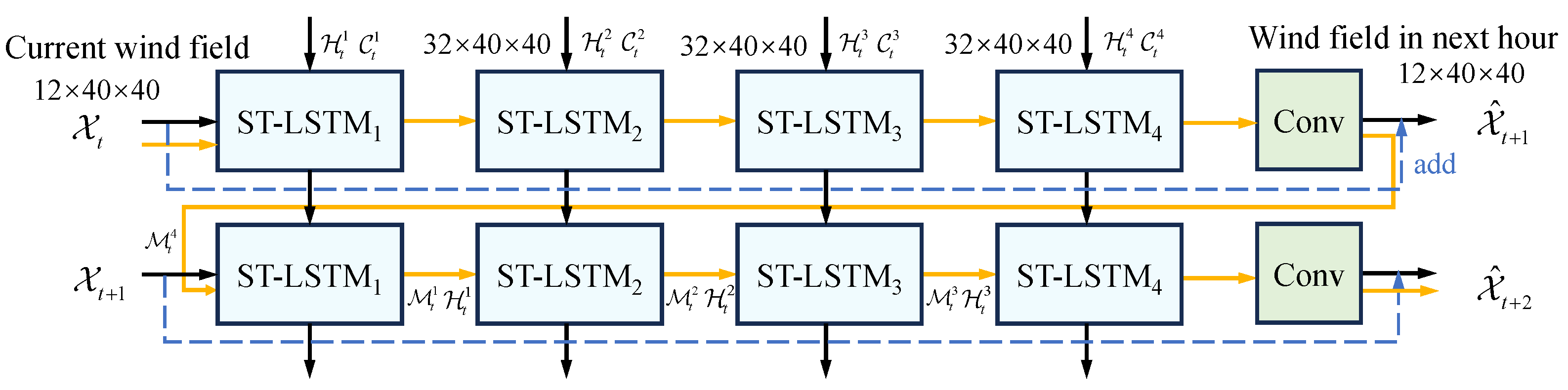
PredRNN introduced Spatiotemporal LSTM (ST-LSTM), which induced a spatiotemporal memory flow. This flow traverses the network in a zigzag pattern, allowing for more efficient communication between layers and enabling joint modeling of spatial correlations and temporal dynamics. This joint modeling is critical for accurately predicting complex spatiotemporal data like wind speed. Figure 1 illustrates the architecture of PredRNN, showing the flow of information through the network’s memory cells.

The loss function in PredRNN includes two main components: the frame reconstruction loss and the memory decoupling loss. These are combined to ensure that the model accurately predicts future frames while preventing redundant features between the memory cells. The frame reconstruction loss ensures that the predicted frames are close to the ground truth. This is typically implemented as the Mean Squared Error (MSE) between the predicted frame and the ground truth frame, as follows:

$$L_{\mathrm{recon}}=\sum _{t=1}^T{∥{\widehat{X}}_t-X_t∥}_2^2$$

(1)

where T is the length of the input sequence, ${\widehat{X}}_t$ is the wind speed forecast at time step t, $X_t$ is the true wind field, and ${∥·∥}_2$ represents the squared Euclidean norm.

A memory decoupling loss is employed to prevent redundancy between the two memory cells within the ST-LSTM unit. This loss maximizes the diversity of memory representations, enabling the model to focus on distinct aspects of spatiotemporal variations. Additionally, the cosine similarity is utilized to maximize the orthogonality between their updates $\Delta {\mathcal{C}}_t^l$ and $\Delta {\mathcal{M}}_t^l$, as follows:

$$L_{\mathrm{decouple}}=\sum _{t=1}^T\sum _{l=1}^L\sum _{c=1}^C{\displaystyle \frac{\left|{\langle \Delta {\mathcal{C}}_t^l,\Delta {\mathcal{M}}_t^l\rangle }_c\right|}{\parallel \Delta {\mathcal{C}}_t^l{\parallel }_c{\parallel \Delta {\mathcal{M}}_t^l\parallel }_c}}$$

(2)

where L is the number of layers in the network, C is the number of channels, ${\langle \Delta {\mathcal{C}}_t^l,\Delta {\mathcal{M}}_t^l\rangle }_c$ is the dot product between the memory updates of ${\mathcal{C}}_t^l$ and ${\mathcal{M}}_t^l$ for channel c, and $\parallel \Delta {\mathcal{C}}_t^l{\parallel }_c$ and $\parallel \Delta {\mathcal{M}}_t^l{\parallel }_c$ are the norms of the memory updates.

For wind speed forecasting, PredRNN predicts the residual of the wind field instead of the wind field directly. The predicted wind field is computed as the sum of the current state and the residual output, improving the model’s accuracy and enabling deeper networks [22].

2.2. ResNet

ResNet has demonstrated significant effectiveness in deep learning tasks, particularly in optimizing efficiency and accuracy as layer depth increases [22]. The architecture leverages skip connections, allowing the model to learn residuals instead of directly learning transformations. These skip connections bypass one or more layers, enabling gradients to flow more effectively through the network, thereby alleviating the vanishing gradient problem.

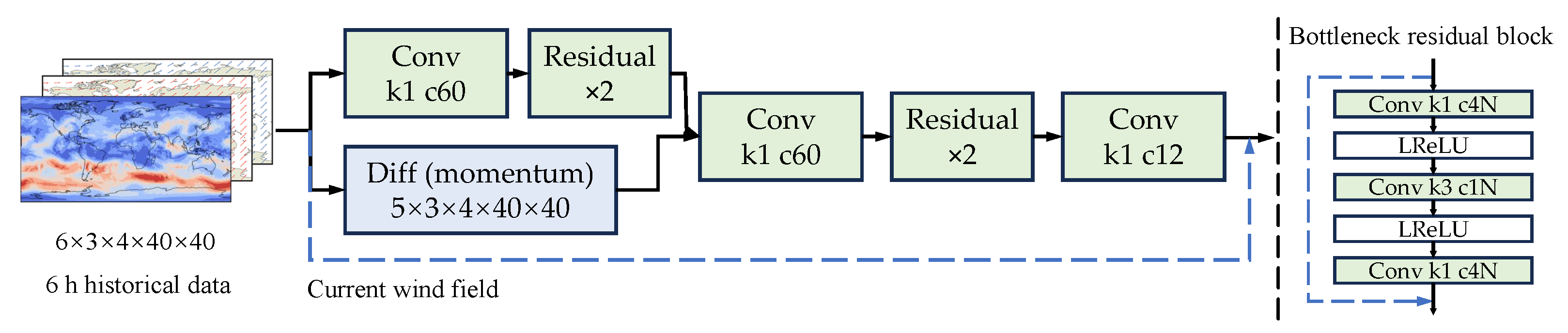
Figure 2 (right) illustrates the architecture of the ResNet model. A bottleneck residual block is employed to reduce computational cost while maintaining high accuracy. The first convolution reduces the number of channels, the second $3\times 3$ convolution extracts spatiotemporal features, and the third restores the original number of channels.

The wind field demonstrates temporal and spatial relationships with historical data and exhibits gradual changes in the stratosphere. As a result, forecasting the residual between the current and subsequent hourly wind states enhances performance significantly. Furthermore, ResNet utilizes features derived from temporal differences to predict this residual in Figure 2 (left), which captures the “momentum” of wind speed. The differences function similarly to the hidden states in PredRNN.

During inference, data from the past 6 h are used iteratively to predict the wind field for the next hour. Compared with RNN-based models, ResNet does not have hidden states, making it faster and easier to train. Additionally, ResNet’s use of more historical data helps in improving prediction accuracy over longer time frames.

2.3. Implementation and Training Detail

Both models were trained using the ERA5 dataset, a comprehensive global reanalysis of climate and atmospheric data [23]. The dataset includes three-dimensional wind velocity at pressure levels of 30, 50, 70, and 100 hPa across two geographical regions, as shown in Figure 3. The input consists of wind velocity data across five dimensions: time sequence, velocity components, pressure levels, and geographical coordinates (latitude and longitude).

The main parameters of PredRNN and ResNet are summarized in

Table 1. The parameters of PredRNN and ResNet.

Type	PredRNN	ResNet
Loss function	Equation (1) + (2)	Equation (1)
Input size	$1\times 4\times 3\times 40\times 40$	$6\times 4\times 3\times 40\times 40$
Output size	$1\times 4\times 3\times 40\times 40$
Training sequence length	6
Optimizer	Adam
Learning rate	Cosine, the initial condition is 0.003
Epochs	10
Batches (Region 1)	138	70
Batches (Region 2)	69	35
Batch Size	32	64

.

Since the ERA5 dataset has a grid resolution of 0.25°, precise wind velocity at specific points requires interpolation. This is achieved through four-dimensional linear interpolation on latitude, longitude, pressure height, and time parameters to derive accurate wind field estimations.

2.4. Prediction Errors of Wind Speed

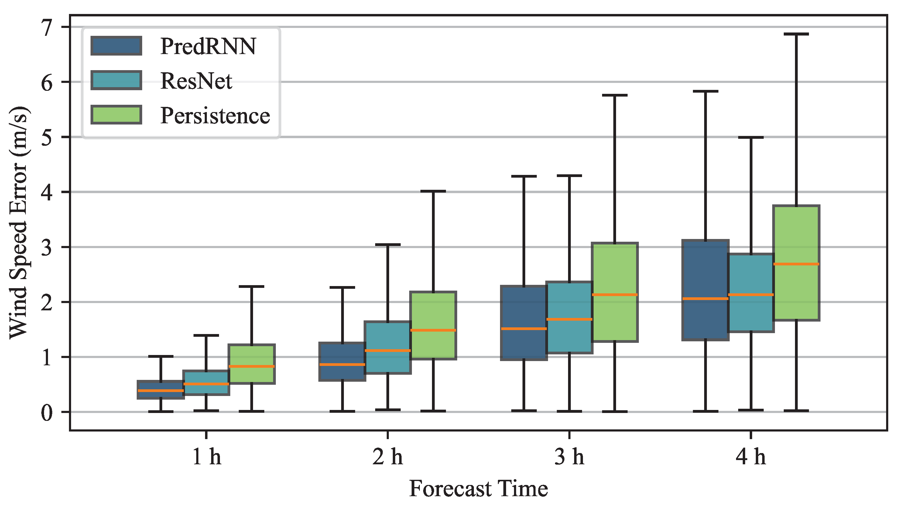
The absolute prediction errors for wind speed over time, using PredRNN, ResNet, and a persistence model (which uses the current wind field as the forecast), are shown in Figure 4. As time progresses, prediction accuracy declines across all models. Each box in the figure represents the interquartile range of the data, with the line inside the box indicating the median value, and the whiskers showing the maximum error.

For 1 h predictions, the median error is 4.8% for PredRNN, 6.1% for ResNet, and 10.0% for the persistence model, with corresponding maximum errors of 12.4%, 17.1%, and 27.9%. As the prediction horizon extends to 4 h, the average error rises to 25.3%, 26.2%, and 33.0%, respectively. Despite this deterioration, both PredRNN and ResNet exhibit approximately 5% greater accuracy compared with the persistence model, suggesting that neural networks enhance wind prediction performance.

While PredRNN achieves the lowest median error overall, ResNet outperforms in terms of the maximum error for 4 h predictions. This difference might be due to the accumulation of errors in PredRNN’s hidden states over extended periods.

3. Balloon Dynamic Model and Energy Model

The balloon is regarded as a particle model, and the states include position $\mathit{x}=[x,y,z]$ and velocity ${\mathit{v}}_{balloon}=[v_x,v_y,v_z]$ in an East–North–Up (ENU) frame, weight of air $m_{air}$, and state of charge (SOC). The following are assumed:

• The ENU frame is an inertial frame and the origin located at the station-keeping target;
• The volume of the balloon remains constant;
• The temperature of the balloon is equivalent to that of the local air;
• The 1976 US standard atmosphere model [24] is utilized for the pressure $p_{local}\left(z\right)$, temperature $T\left(z\right)$, density $\rho \left(z\right)$ and viscosity of air $\mu \left(z\right)$.

3.1. Dynamics

System weight $m_{total}$ includes helium $m_{He}$, air $m_{air}$, and structure $m_{structure}$ items, as follows:

$$m_{total}=m_{He}+m_{air}+m_{structure}$$

(3)

The external forces on the balloon include buoyancy, gravity, aerodynamic drag, and the momentum exchange with the surrounding air due to differential mass flow. Because of the large volume of the balloon, its movement drives the surrounding air; thus the added-mass effect is significant. The dynamic formula is as follows:

$$(m_{total}+C_{V}V\rho )\mathit{a}=-\rho \mathit{g}V+m_{total}\mathit{g}+{\displaystyle \frac{1}{2}}{C}_D\rho {\mathit{v}}_r\left|v_r\right|V^{{\displaystyle \frac{2}{3}}}-{\dot{m}}_{air}{\mathit{v}}_{balloon}$$

(4)

where $C_V$ is the added-mass factor, V is the volume of the balloon, the gravity coefficient is $g=9.8$ N/kg ${\mathit{v}}_r={\mathit{v}}_{wind}-{\mathit{v}}_{balloon}$, and ${\mathit{v}}_r$ and ${\mathit{v}}_{wind}$ are the wind relative velocity and wind absolute velocity in the ENU frame.

The drag coefficient $C_D$ of the balloon is estimated using an empirical formula derived from the aerodynamics of a ball [25].

$$\begin{array}{c}\hfill \left\{\begin{array}{c}\begin{array}{ccc}\hfill C_D& ={\displaystyle \frac{24}{Re}}+{\displaystyle \frac{6}{1+\sqrt{Re}}}+0.4,\hfill & \hfill Re<2.7\times {10}^5\\ \hfill lg{C}_D& =25.821-4.825lgRe,\hfill & \hfill 2.7\times {10}^5<Re<3.7\times {10}^5\\ \hfill lg{C}_D& =-0.699-0.347e^{-38.533{\left(lg{\displaystyle \frac{Re}{3.7\times {10}^5}}\right)}^{5.306}},\hfill & \hfill 3.7\times {10}^5<Re<{10}^6\\ \hfill C_D& =0.2,\hfill & \hfill otherwise\end{array}\hfill \end{array}\right.\end{array}$$

(5)

where $Re={\displaystyle \frac{\rho v_{r}d}{\mu }}$ is the Reynolds number of the balloon, d is the diameter of the balloon.

The altitude control of stratospheric balloons primarily relies on the operation of valves and pumps. The model for the valve and pump system is described as follows:

$${\displaystyle \frac{\mathrm{d}{m}_{air}}{\mathrm{d}t}}=\left\{\begin{array}{cc}-A_{valve}c\sqrt{2\Delta p\rho },\hfill & u=-1\hfill \\ 0,\hfill & u=0\hfill \\ {\displaystyle \frac{P_{pump}{\eta }_{pump}}{\Delta p\rho }},\hfill & u=1\hfill \end{array}\right.$$

(6)

where $A_{valve}$ is the area of the valve, c is the valve flow coefficient, $P_{pump}$ is the power of the pump, and ${\eta }_{pump}$ is the efficiency of the pump.

The difference of pressure $\Delta p$ and the internal pressure of the balloon $p_{internal}$ are

$$\left\{\begin{array}{c}{p}_{internal}=({\displaystyle \frac{m_{He}}{M_{He}}}+{\displaystyle \frac{m_{air}}{M_{air}}}){\displaystyle \frac{RT}{V}}\hfill \\ \Delta p=p_{internal}-p_{local}\hfill \end{array}\right.$$

(7)

where the molar mass of air $M_{air}$ is 28.9644 g/mol, the molar mass of helium $M_{He}$ is 4.003 g/mol, and the gas constant R is 8.31432 J.

3.2. Energy Model

The power consumption comprises pump ($P_{pump}=$ 100 W) and payload ($P_{payload}=$ 200 W), while electricity is generated by solar panels ($P_{solar}$), as follows:

$${\displaystyle \frac{\mathrm{d}SOC}{\mathrm{d}t}}={\displaystyle \frac{P_{solar}-P_{pump}-P_{payload}}{E}}$$

(8)

where the total battery capacity E is 3500 Wh.

A stratospheric aircraft solar power model was studied in [26,27]. It is assumed that the power generated by the balloon is independent of the balloon attitude, the solar panels are placed horizontally, and a simplified Earth precession model is used, as follows:

$$sinh=sin\delta sin\varphi +cos\delta cos\omega cos\varphi$$

(9)

where $\delta$ is declination, $\varphi$ is latitude, $\omega$ is solar time angle.

Declination moves between the Tropic of Cancer, as follows:

$$\delta =23.45sin\left(2\pi {\displaystyle \frac{284+n}{365}}\right)$$

(10)

where n is the days since 1 January of this year.

The following formula is used for the approximation of the solar time angle $\omega$:

$$\omega ={\displaystyle \frac{\pi }{12}}\left(t_{UTC}-12\right)+l$$

(11)

where l is longitude. $t_{UTC}$ is the hours of UTC since the day.

The solar irradiation intensity is

$$I_D={\tau }_{atm}{I}_{0}sin\left(h\right)$$

(12)

The average solar radiation intensity $I_0=1367$ W, ${\tau }_{atm}$ is the atmospheric transmission coefficient, and the formula is

$$\left\{\begin{array}{c}{\tau }_{atm}=0.5\sqrt{exp\left(-0.65m_{air}\right)+exp\left(-0.095m_{air}\right)}\hfill \\ m_{air}={\displaystyle \frac{p_{local}\left(z\right)}{p_{local}\left(0\right)}}\left[\sqrt{1229+614{sin}^2\left(h\right)}-614sin\left(h\right)\right]\hfill \end{array}\right.$$

(13)

For this work, the necessary simulation parameters are selected, as shown in

Table 2. Parameters of balloons in the simulation.

Type	Symbol	Value	Unit
Structure mess	$m_{structure}$	177	kg
Helium mess	$m_{He}$	31.6	kg
Volume	V	4211.3	m3
Diameter	d	20	m
Added-mess factor	$C_V$	0.5
Valve diameter	$d_{vavle}$	120	mm
Valve flow coefficient	c	0.3
Power of pump	$P_{pump}$	100	W
Efficiency of pump	${\eta }_{pump}$	50%
Capacity of battery	E	3500	Wh
Solar panel area	$A_{solar}$	3.5	m2
Efficiency of solar	${\eta }_{solar}$	18%
Min differential pressure	$min\Delta p$	50	Pa
Max differential pressure	$max\Delta p$	500	Pa
Min SOC	$minSOC$	10%

.

4. Simultaneous Optimistic Optimization for Planning and Reward Function Design

Optimistic optimization is a numerical method for optimizing black-box functions, which assumes that the target function is Lipschitz continuous under a constant L. This means that, for any two points $x_1$ and $x_2$ in the domain $\mathcal{X}$, the following inequality holds:

$$\left|\right|f\left(x_1\right)-f\left(x_2\right)\left|\right|\le L\left|\right|x_1-x_2\left|\right|$$

(14)

Figure 5 illustrates the key principle of this method. The curve represents the unknown function $f\left(x\right)$ to be optimized, and the red sample points $\left\{x_i\right\}$ are known. The dotted line indicates the upper bound on the function as derived from the Lipschitz condition. As more sample points are added, the upper bound approaches the true function $f\left(x\right)$.

The primary ideas behind this method are as follows:

• The Lipschitz condition is used to approximate the true distribution of the function through its upper bound.
• A strategy, such as bisection, is employed to select points for expansion. This approach explores the distribution while efficiently approaching its maximum value.

The term “Optimistic” refers to the method’s reliance on the upper bound to guide the selection of points.

Contrary to the requirement of Lipschitz L, SOO introduces a function $h_{max}\left(t\right)$, which limits the maximum depth of the search tree after t expansions. To identify the maximum point of $f\left(x\right)$, SOO expands all the leaves $(h,j)$ of the current tree simultaneously at each round, where h is the depth and j is the index of the leaf nodes. The selection criterion for expansion is the existence of a semi-metric l such that the corresponding upper bound $b\left(x_{h,j}\right)$ could be the highest. In other words, all cells potentially to be optimal are selected [17], as follows:

$$b\left(x_{h,j}\right)=f\left(x_{h,j}\right)+\underset{x\in X_{h,j}}{sup}l(x_{h,j},x)$$

(15)

where $h_{max}\left(t\right)=\sqrt{t}$ in this work.

4.1. Simultaneous Optimistic Optimization for Planning

The objective of the balloon controller is to optimize the sequence of control inputs $\left\{u_i\right\}$, to maximize the value function $V\left(x_0\right)$, which is different from the typical function optimization. In function optimization, the process involves splitting corresponding squares into 2D squares of half length. In contrast, in trajectory planning, the search tree grows according to the action sequence. The value function is defined as

$$V\left(x_0\right)=\sum _{t=0}^N{\gamma }^{t}r\left(x_t\right)$$

(16)

Here, the discounted factor $\gamma$ is 0.99, and $r\left(x_t\right)$ represents the reward function at time step t.

Since networks provide short-term wind predictions, a receding horizon control strategy is adopted. This strategy involves re-planning the valve and pump actions every 30 min for the next 3.5 to 4 h, with the first action in the sequence being executed immediately.

Safety and power constraints are critical considerations in the proposed approach. Specific rules are enforced to ensure that the balloon remains superpressured ($\Delta p>50$ Pa), maintain the SOC above 10%, and prevent structural damage ($\Delta p<500$ Pa).

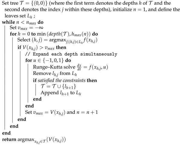
Consequently, the planning algorithm deviates from the SOO framework as outlined in Algorithm 1.

Algorithm 1: Simultaneous Optimistic Optimization for Planning

4.2. Reward Function

The reward function evaluates the value of state and action, promoting improved station-keeping performance and reduced power consumption. Typically, differences in power consumption are integrated into the reward function. However, as balloons are equipped with solar panels for power generation, the SOC is incorporated instead, as follows:

$$r\left(\mathit{x}\right)={\displaystyle \frac{1+e^{-1}}{1+exp(\frac{\left|\right|\mathit{x}\left|\right|}{50km}-1)}}SO{C}^n$$

(17)

where $r\in [0,1]$ and $n\in (0,1)$; $n=0.5$ in this study. This reward function resembles a sigmoid curve: it encourages the balloon to approach the station when it is far away, while maintaining a flat curve when the balloon is near the station. Additionally, $\sqrt{SOC}$ promotes energy-consuming actions when energy is abundant and energy-saving actions when it is scarce.

If two action sequences result in the same trajectory, the difference in reward is

$$\Delta r\left(\mathit{x}\right)=c[{(SO{C}_0+\Delta SOC)}^n-SO{C}_0^n]=c\left[nSO{C}_0^{n-1}\Delta SOC\right]+o(\Delta SOC)$$

(18)

When power consumption $\Delta SOC$ is equal, $\Delta r\left(\mathit{x}\right)$ is determined by $nSO{C}_0^{n-1}$. Thus, $n\in (0,1)$ satisfies the requirements. Furthermore, adjusting n can balance station-keeping performance and energy consumption effectively.

4.3. Baseline Algorithms: Greedy and A*

The Greedy and A* algorithms [28] are used as baseline methods. The Greedy algorithm selects the action that yields the highest immediate reward in the current state without accounting for future consequences or exploring alternative options, as follows:

$$u={\mathrm{argmax}}_{u\in \{-1,0,1\}}r(x,u)$$

(19)

In contrast, the A* algorithm employs a loss function as its optimization target. The loss of an action $a_i$ is defined as $1-r(x_i,a_i)$, and the loss of an entire action sequence is expressed as

$$\widehat{Q}(x,a)=\sum _{i=1}^n(1-r(x_i,a_i))+(N-n)(1-r(x,a))$$

(20)

The first term represents the cumulative loss of the previous action sequence, while the second term is the heuristic function, which estimates the remaining loss from the current state to the target. In this heuristic, it is assumed that the balloon remains stationary, with the loss multiplied by the remaining sequence length $N-n$.

It should be noted that this heuristic function underestimates the total loss and is not monotonic. Additionally, the solution provided by Equation (20) is not guaranteed to be optimal.

5. Simulation Results

5.1. Planning in Constrained State Space

Figure 6 illustrates the result of a balloon launched from position 2 (15° N, 112° E) on 20 March 2023 at 14:00 UTC, utilizing true wind data to assess planning capabilities. The blue area denotes the restricted flight zone, while the grey tree depicts the potential trajectories explored. The line indicates that the controller, through various expansion efforts, seeks to identify an optimal trajectory that avoids entering restricted zones. The SOOP algorithm prunes nodes from the tree when the path intersects the restricted flight zone, demonstrating the balloon’s capacity to navigate around the restricted area throughout the entire flight while achieving optimality.

In the right panel of Figure 6, it is apparent that, due to finite receding horizons, SOOP with fewer expansion times results in a higher $V\left(x\right)$ in the short term. Conversely, SOOP with more expansion times benefits from extended receding horizons, leading to a higher $V\left(x\right)$ over the long term. For the 4 h prediction, expanding all actions requires $3^8=6561$ computations; in contrast, SOOP only necessitates 64, as $h_{max}\left(t\right)=\sqrt{t}$. Thus, SOOP efficiently balances exploration and exploitation, with a time complexity of $O\left(t^2\right)$.

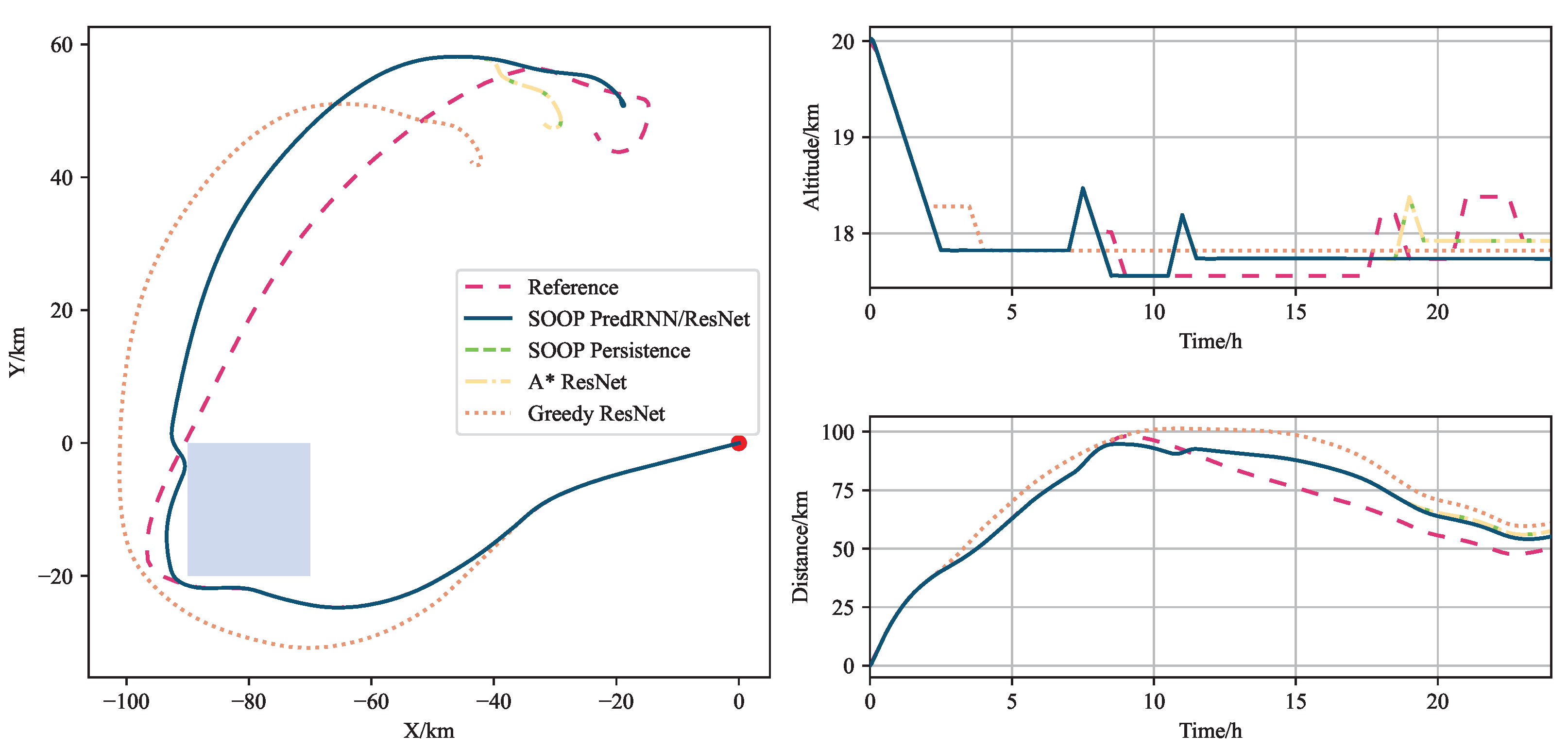
In Figure 7, the balloon is launched from position 1 (40° N, 100° E) on 1 August 2023 at 14:00 UTC. It shows the trajectory in the horizon panel, altitude, and distance to the origin with different networks and control methods. These trajectories illustrate how the balloon navigates around the restricted flight zone while attempting to maintain proximity to the station. Initially, the SOOP method closely follows the reference trajectory, but its performance declines after approximately 10 h. This degradation is attributed to the limited planning horizon of the SOOP controller, which is constrained to 4 h. Despite this limitation, SOOP still outperforms the greedy algorithm.

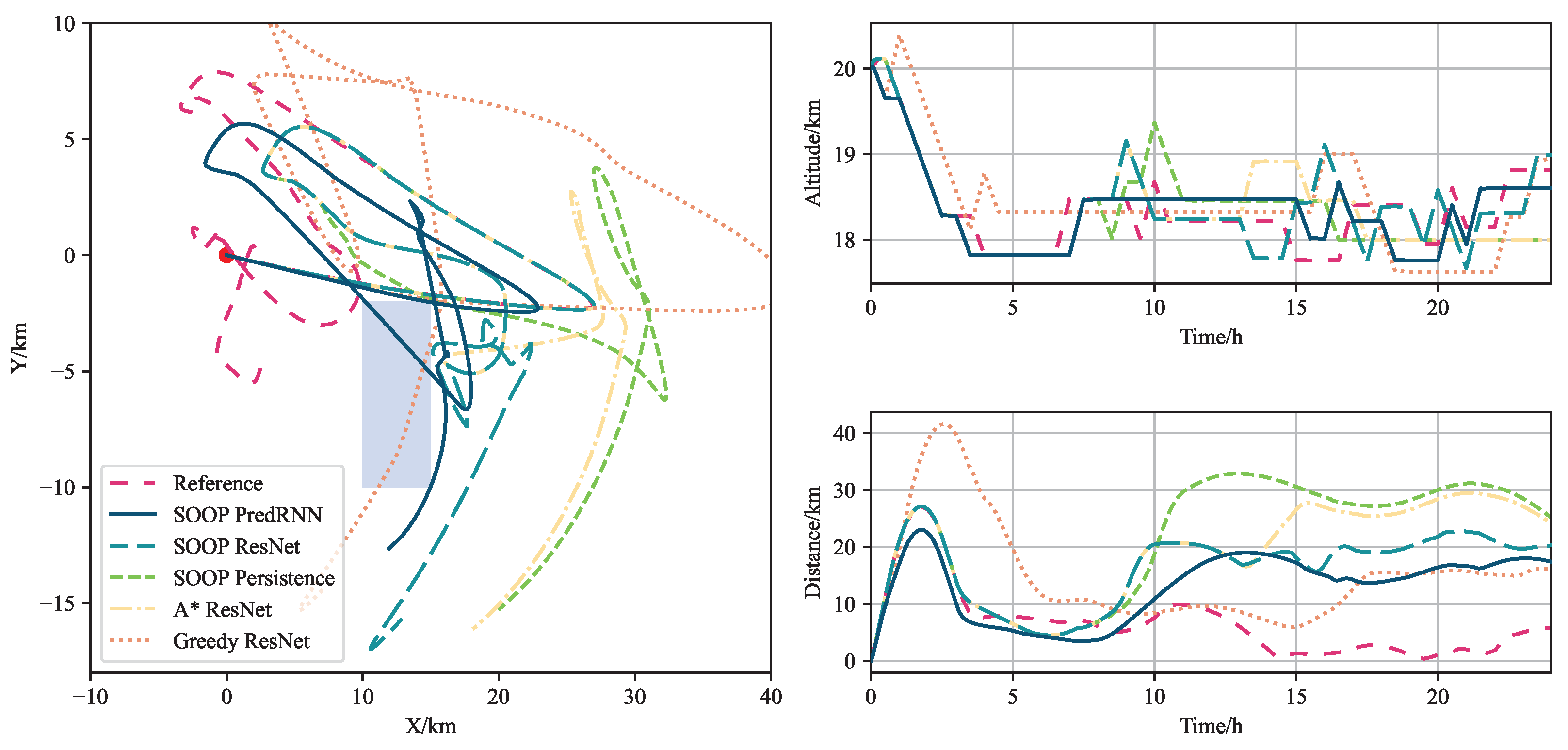
Figure 8 shows the trajectories at position 2. In the Figure 8 (left), the reference trajectory maintains a radius of approximately 10 km from the station. The SOOP controller, using PredRNN, achieves a distance of less than 20 km, while the SOOP method based on ResNet maintains a radius of around 20 km. However, the SOOP method using persistence and the A* algorithm with ResNet performs the worst, with a radius of approximately 30 km. The greedy method initially reaches up to 40 km before returning to within 20 km. Thus, station-keeping performance depends not only on the control methods but also on the wind distribution.

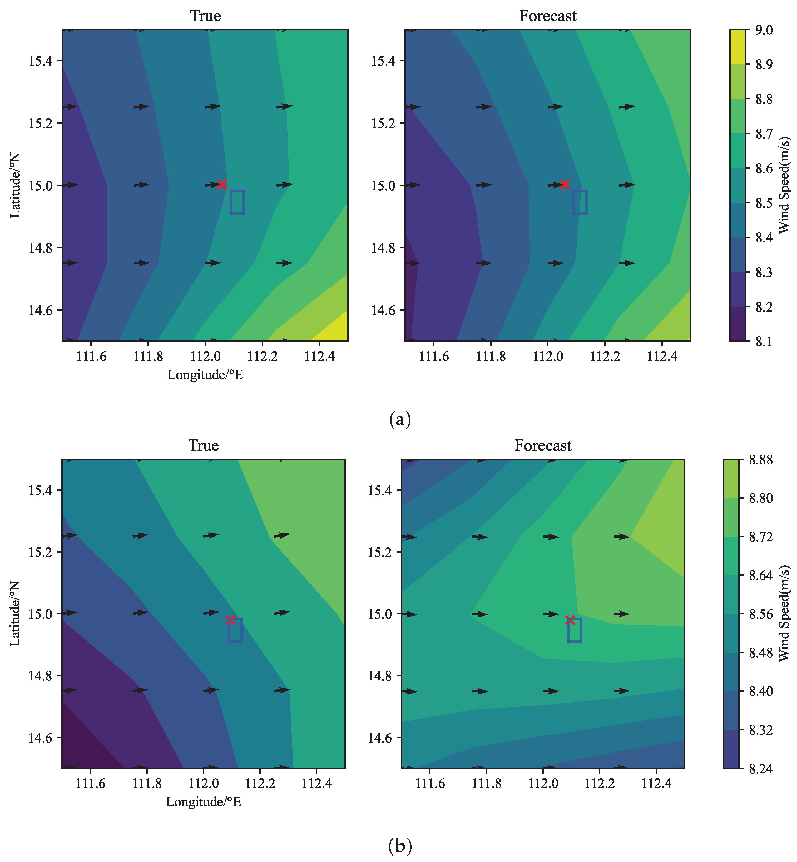
SOOP with PredRNN and the greedy method violate the flight constraints by flying into the restricted area. Figure 9a,b depict the true wind fields at 09:00 and 10:00 UTC, respectively, alongside forecast wind fields generated at 08:00 UTC. The cross markers indicate the balloon’s true positions at 09:00 and 10:00 UTC, while the blue square represents the restricted area, and the arrows indicate wind direction. Despite the wind forecast generated by PredRNN having an error of less than 1 m/s, the wind’s direction remains consistent. Therefore, the primary cause of the balloon entering the restricted area is the absence of suitable winds to steer it away. In contrast, both the reference and the SOOP method using ResNet manage to successfully avoid the restricted area.

These results reveal the significant impact of finite receding horizons and wind distribution on the controller’s performance. Errors in the wind prediction provided by PredRNN, particularly in the 4 h forecast window, restrict the controller’s effectiveness, leading to suboptimal trajectory planning.

5.2. Launch in Different Time

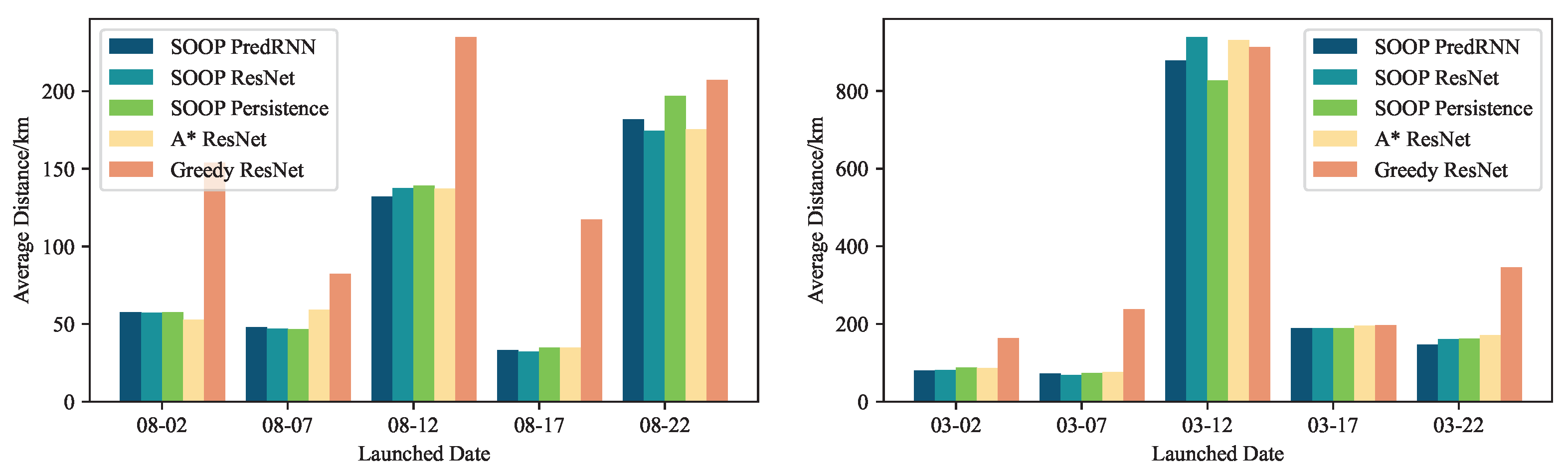
The impact of launch date on the average distance between balloons and their target station has been analyzed for various planning methods, as illustrated in Figure 10. This analysis evaluates the influence of both flight date and launch position. The observed average distances from the station vary significantly, ranging from 30 km to 800 km. Notably, certain launch dates prove unsuitable for flight operations—12 August and 22 August for position 1 and 12 March for position 2—as the average distance is greater than 100 km.

The SOOP method exhibits superior average station-keeping capability when compared with both A* and the greedy algorithm. In the 10 cases examined, PredRNN enhances performance in 7 instances while showing minor degradation in 2 cases. Furthermore, PredRNN and ResNet display varying levels of performance across different scenarios, attributable to their differing accuracies in short-term and long-term predictions. These findings suggest that SOOP outperforms A* and greedy algorithms. While neural networks generally improve performance in most scenarios, their impact on short-range and long-range capabilities varies case by case.

5.3. Long Duration Flight

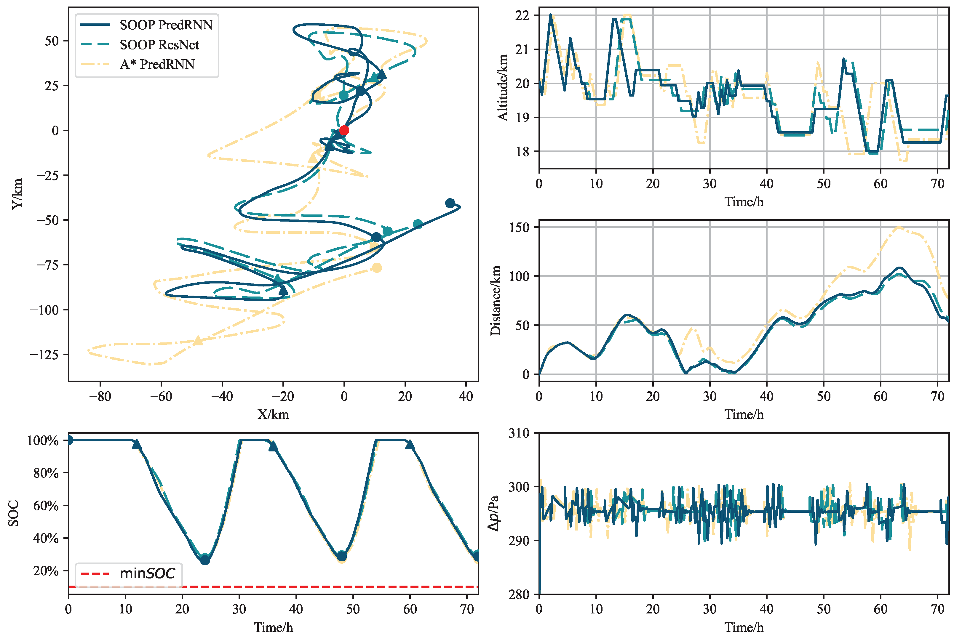
Figure 11 presents the trajectories, SOC, and $\Delta p$ for a balloon launched at position 2 on 22 March 2023 over a 3-day period. The energy management and pressure requirements are successfully maintained throughout the duration. Data points are plotted at 12 h intervals, with triangles denoting sunset and circles indicating sunrise. Notably, the balloon’s movement pattern exhibits an eastward trajectory at sunrise and a westward path in the afternoon. This behavior optimizes sunlight capture in the morning and extends the duration of electricity generation in the afternoon, underscoring the significant influence of SOC in the reward function.

The SOOP method with PredRNN demonstrated better performance for the initial 63 h. Subsequently, the SOOP method utilizing the persistence model achieved the best results. This observation suggests that employing a more accurate forecast model does not guarantee optimal performance consistently. The finite receding horizons and wind distribution may lead to suboptimal methods occasionally yielding better outcomes. Furthermore, the absence of southerly winds resulted in a periodic east–west movement, indicating that this particular date may not be suitable for flight operations.

Figure 12 illustrates the trajectories, SOC, and $\Delta p$ for a balloon launched at position 1 on 7 August. This scenario reveals two distinct flight patterns. Initially, the methods leveraged different wind directions to enhance performance. The balloon first traveled up to 50 km away before approaching the station during the 25–35 h period. Subsequently, due to the absence of reversing winds in the north–south direction, the balloon adopted a periodic movement between west and east.

6. Conclusions

This study introduced a novel receding horizon control approach based on optimistic optimization to enhance station-keeping performance under various constraints. Wind field forecasts, generated by PredRNN or ResNet, were utilized for action planning. The problem was formulated as a discretized optimal control problem with constraints, enabling the solution to address complex environmental conditions while satisfying specified constraints. A reward function has been developed to optimize station-keeping performance and manage power consumption effectively.

Extensive simulations have validated the effectiveness of the proposed approach. The results demonstrate significant improvements in computational efficiency and performance compared with traditional techniques such as greedy and A* algorithms. Neural network integration has shown slight performance enhancements, although the impact varies across different scenarios. It is noteworthy that the employment of a more accurate forecast model and SOOP does not consistently guarantee optimal performance.

The achievement of optimal station-keeping performance is heavily dependent on wind field characteristics and the range of receding horizons. Future research directions should integrate wind field physical constraints to improve wind forecasting accuracy and consider thermodynamics with solar radiation. Furthermore, the proposed method has potential applications in long-range balloon trajectory planning, and the corresponding accessibility conditions should be investigated.

References

- Arum, S.C.; Grace, D.; Mitchell, P.D. A review of wireless communication using high-altitude platforms for extended coverage and capacity. Comput. Commun. 2020, 157, 232–256. [Google Scholar] [CrossRef]
- Karabulut Kurt, G.; Khoshkholgh, M.G.; Alfattani, S.; Ibrahim, A.; Darwish, T.S.J.; Alam, M.S.; Yanikomeroglu, H.; Yongacoglu, A. A Vision and Framework for the High Altitude Platform Station (HAPS) Networks of the Future. IEEE Commun. Surv. Tutor. 2021, 23, 729–779. [Google Scholar] [CrossRef]
- Bellemare, M.G.; Candido, S.; Castro, P.S.; Gong, J.; Machado, M.C.; Moitra, S.; Ponda, S.S.; Wang, Z. Autonomous navigation of stratospheric balloons using reinforcement learning. Nature 2020, 588, 77–82. [Google Scholar] [CrossRef] [PubMed]
- Sniderman, A.C.; Broucke, M.E.; D’Eleuterio, G.M.T. Formation control of balloons: A block circulant approach. In Proceedings of the 2015 American Control Conference (ACC), Chicago, IL, USA, 1–3 July 2015; pp. 1463–1468. [Google Scholar] [CrossRef]
- Vandermeulen, I.; Guay, M.; McLellan, P.J. Distributed Control of High-Altitude Balloon Formation by Extremum-Seeking Control. IEEE Trans. Control Syst. Technol. 2018, 26, 857–873. [Google Scholar] [CrossRef]
- Rossi, F.; Saboia, M.; Krishnamoorthy, S.; Hook, J.V. Proximal Exploration of Venus Volcanism with Teams of Autonomous Buoyancy-Controlled Balloons. Acta Astronaut. 2023, 208, 389–406. [Google Scholar] [CrossRef]
- Ding, Y. Data Science for Wind Energy, 1st ed.; Chapman and Hall/CRC: Boca Raton, FL, USA, 2019. [Google Scholar] [CrossRef]
- Bonev, B.; Kurth, T.; Hundt, C.; Pathak, J.; Baust, M.; Kashinath, K.; Anandkumar, A. Spherical Fourier Neural Operators: Learning Stable Dynamics on the Sphere. arXiv 2023, arXiv:2306.03838. [Google Scholar]
- Lam, R.; Sanchez-Gonzalez, A.; Willson, M.; Wirnsberger, P.; Fortunato, M.; Alet, F.; Ravuri, S.; Ewalds, T.; Eaton-Rosen, Z.; Hu, W.; et al. Learning skillful medium-range global weather forecasting. Science 2023, 382, 1416–1421. [Google Scholar] [CrossRef]
- Kochkov, D.; Yuval, J.; Langmore, I.; Norgaard, P.; Smith, J.; Mooers, G.; Klöwer, M.; Lottes, J.; Rasp, S.; Düben, P.; et al. Neural general circulation models for weather and climate. Nature 2024, 632, 1060–1066. [Google Scholar] [CrossRef]
- Trebing, K.; Stanczyk, T.; Mehrkanoon, S. SmaAt-UNet: Precipitation nowcasting using a small attention-UNet architecture. Pattern Recognit. Lett. 2021, 145, 178–186. [Google Scholar] [CrossRef]
- Ravuri, S.; Lenc, K.; Willson, M.; Kangin, D.; Lam, R.; Mirowski, P.; Fitzsimons, M.; Athanassiadou, M.; Kashem, S.; Madge, S.; et al. Skilful precipitation nowcasting using deep generative models of radar. Nature 2021, 597, 672–677. [Google Scholar] [CrossRef]
- Zhang, Y.; Long, M.; Chen, K.; Xing, L.; Jin, R.; Jordan, M.I.; Wang, J. Skilful nowcasting of extreme precipitation with NowcastNet. Nature 2023, 619, 526–532. [Google Scholar] [CrossRef] [PubMed]
- Acikgoz, H.; Budak, U.; Korkmaz, D.; Yildiz, C. WSFNet: An efficient wind speed forecasting model using channel attention-based densely connected convolutional neural network. Energy 2021, 233, 121121. [Google Scholar] [CrossRef]
- Wang, Y.; Zou, R.; Liu, F.; Zhang, L.; Liu, Q. A review of wind speed and wind power forecasting with deep neural networks. Appl. Energy 2021, 304, 117766. [Google Scholar] [CrossRef]
- Shahriari, B.; Swersky, K.; Wang, Z.; Adams, R.P.; De Freitas, N. Taking the Human Out of the Loop: A Review of Bayesian Optimization. Proc. IEEE 2016, 104, 148–175. [Google Scholar] [CrossRef]
- Munos, R. From Bandits to Monte-Carlo Tree Search: The Optimistic Principle Applied to Optimization and Planning. Found. Trends® Mach. Learn. 2014, 7, 1–129. [Google Scholar] [CrossRef]
- Wang, Z.; Shakibi, B.; Jin, L.; Freitas, N. Bayesian Multi-Scale Optimistic Optimization. In Proceedings of the Seventeenth International Conference on Artificial Intelligence and Statistics PMLR, Reykjavik, Iceland, 22–25 April 2014; pp. 1005–1014, ISSN 1938–7228. [Google Scholar]
- Buşoniu, L.; Páll, E.; Munos, R. Continuous-action planning for discounted infinite-horizon nonlinear optimal control with Lipschitz values. Automatica 2018, 92, 100–108. [Google Scholar] [CrossRef]
- Wang, Y.; Wu, H.; Zhang, J.; Gao, Z.; Wang, J.; Yu, P.S.; Long, M. PredRNN: A Recurrent Neural Network for Spatiotemporal Predictive Learning. IEEE Trans. Pattern Anal. Mach. Intell. 2023, 45, 2208–2225. [Google Scholar] [CrossRef]
- Bao, Y.; Shen, Q.; Cao, Y.; Ding, W.; Shi, Q. Residual attention enhanced Time-varying Multi-Factor Graph Convolutional Network for traffic flow prediction. Eng. Appl. Artif. Intell. 2024, 133, 108135. [Google Scholar] [CrossRef]
- He, K.; Zhang, X.; Ren, S.; Sun, J. Deep Residual Learning for Image Recognition. In Proceedings of the 2016 IEEE Conference on Computer Vision and Pattern Recognition (CVPR), Las Vegas, NV, USA, 27–30 June 2016; pp. 770–778. [Google Scholar] [CrossRef]
- Hersbach, H.; Bell, B.; Berrisford, P.; Hirahara, S.; Horányi, A.; Muñoz-Sabater, J.; Nicolas, J.; Peubey, C.; Radu, R.; Schepers, D.; et al. The ERA5 global reanalysis. Q. J. R. Meteorol. Soc. 2020, 146, 1999–2049. [Google Scholar] [CrossRef]
- US Standard Apparel. US Standard Atmosphere; National Oceanic and Atmospheric Administration: Washington, DC, USA, 1976. [Google Scholar]
- Wu, Z. Aerodynamics; Tsinghua University Press: Beijing, China, 2007. [Google Scholar]
- Yang, X.; Liu, D. Renewable power system simulation and endurance analysis for stratospheric airships. Renew. Energy 2017, 113, 1070–1076. [Google Scholar] [CrossRef]
- Gao, X.Z.; Hou, Z.X.; Guo, Z.; Liu, J.X.; Chen, X.Q. Energy management strategy for solar-powered high-altitude long-endurance aircraft. Energy Convers. Manag. 2013, 70, 20–30. [Google Scholar] [CrossRef]
- Russell, S.J.; Norvig, P.; Davis, E. Artificial Intelligence: A Modern Approach, 3rd ed.; Prentice Hall Series in Artificial Intelligence; Prentice Hall: Upper Saddle River, NJ, USA, 2010. [Google Scholar]