Comparative Analysis of Machine Learning Models for Predictive Maintenance of Ball Bearing Systems

Abstract

In the era of Industry 4.0 and beyond, ball bearings remain an important part of industrial systems. The failure of ball bearings can lead to plant downtime, inefficient operations, and significant maintenance expenses. Although conventional preventive maintenance mechanisms like time-based maintenance, routine inspections, and manual data analysis provide a certain level of fault prevention, they are often reactive, time-consuming, and imprecise. On the other hand, machine learning algorithms can detect anomalies early, process vast amounts of data, continuously improve in almost real time, and, in turn, significantly enhance the efficiency of modern industrial systems. In this work, we compare different machine learning and deep learning techniques to optimise the predictive maintenance of ball bearing systems, which, in turn, will reduce the downtime and improve the efficiency of current and future industrial systems. For this purpose, we evaluate and compare classification algorithms like Logistic Regression and Support Vector Machine, as well as ensemble algorithms like Random Forest and Extreme Gradient Boost. We also explore and evaluate long short-term memory, which is a type of recurrent neural network. We assess and compare these models in terms of their accuracy, precision, recall, F1 scores, and computation requirement. Our comparison results indicate that Extreme Gradient Boost gives the best trade-off in terms of overall performance and computation time. For a dataset of 2155 vibration signals, Extreme Gradient Boost gives an accuracy of 96.61% while requiring a training time of only 0.76 s. Moreover, among the techniques that give an accuracy greater than 80%, Extreme Gradient Boost also gives the best accuracy-to-computation-time ratio.

1. Introduction

The study of ball bearings in rotating machines has evolved over time due to technological advancements. Ancient civilisations developed early rotational devices such as waterwheels and windmills [1]. The rise of industrialisation further prompted innovation in rotating machines. These advancements led to the development of more efficient and sophisticated rotating machines with novel applications in various fields, including transportation, manufacturing equipment, domestic equipment, and power production. Ball bearings, consisting of outer and inner rings, a set of balls, and a cage, reduce friction and improve smooth rotation. They are an integral part of any rotating machinery and are responsible for 40 percent of machinery breakdowns [2,3,4]. These breakdowns are associated with their installation, poor maintenance strategy, fatigue, and regular wear.

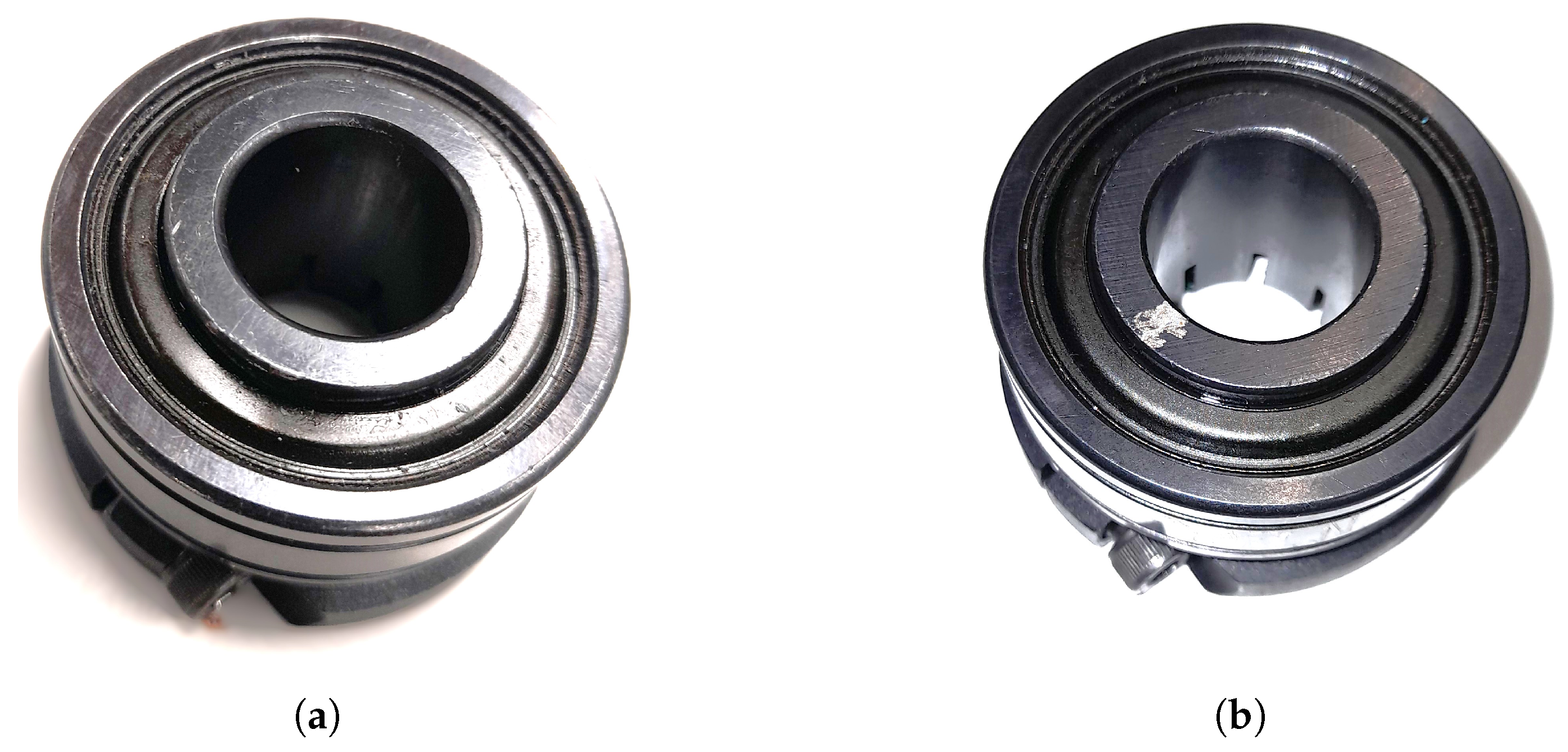
The performance and efficiency of rotating machinery are greatly affected by bearings. Unexpected bearing faults often develop from their installation, maintenance strategy, fatigue, and regular wear, posing diagnostic challenges. These faults can be classified into two categories: distributed defects that affect a wide area, and localised defects that start as single-point defects (ref Figure 1). Inspection techniques like visual checks, ultrasound, and vibration analysis [5] help identify these faults, which is vital for machinery reliability.

Distributed Defects: These defects impact bearings significantly and are challenging to identify based on specific frequency. They occur due to various reasons such as heat, vibrations, noise during operation, production errors, and excessive loads [6]. These faults can cause early rotor system failure or severe damage, making their detection challenging [7]. However, several inspection techniques such as visual observations and non-destructive methods can be employed [5].

Localised Defects: These faults are single-point issues caused by flaws in the manufacturing process, quality of raw material, or fitting errors [8]. Over time, as the bearings age, these localised defects progress and expand, leading to distributed fault patterns. These manifest as distinct vibrations, minimal changes in the load torque, and the emergence of multiple frequencies [9,10]. The distributed and localised defects pose a big problem to the throughput and efficiency of modern rotating machines. A timely identification of these faults can greatly improve the efficiency of rotating machines, and machine learning has a huge role to play in this regard.

By investigating failures, industries can identify weaknesses and refine their designs and manufacturing processes, leading to better quality. When products have defects or fail to meet standards, it results in unhappy customers, a decrease in market share, and increased costs due to quality-related problems such as recalls or repairs [11]. Even brief failures can impact continuous operations, leading to missed deadlines, financial losses, and delayed deliveries. To keep the production line running smoothly and safely, it is essential to have a well-organised system in place that effectively manages all aspects of the equipment, including machines and components. This requires a system that can diagnose potential breakdowns and taking proactive measures to prevent any impending faults or downtime. Implementing preventive measures through condition monitoring systems uncover cost-effective solutions, enhance safety by identifying and minimising hazards, and contribute to product development and innovation by providing valuable insights for iterative improvements. In the past, preventive maintenance techniques like time- and usage-based maintenance, fixed replacement intervals, and manual data analysis have been used. While these traditional methods provided some level of preventive capability, they were often reactive, time-consuming, and imprecise. In future industrial systems, the usage of advanced technologies like Internet of Things (IoT) [12], digital twin [13], and data-driven approaches like big data analytics, machine learning, and cloud computing [14,15,16] are being explored and employed.

Compared to existing manual data analysis techniques, the utilisation of Machine Learning (ML) has the potential to perform the function of forecasting and anticipating malfunctions [17] through the creation of algorithms that can detect patterns from data and use that understanding to make accurate predictions or choices. In particular, machine learning algorithms are very good at recognising anomalies in data, learning from patterns, data analysis, and optimisation of maintenance schedules. In recent years, machine learning [18] has become widely accepted and is being employed in a broad range of applications. There is hardly an area of everyday life where machine learning or deep learning algorithms are not finding their applications. Today, we see their application in fields such as self-driven cars [19], smart management of energy consumption in renewable energy communities [20,21], healthcare, transportation, supply chain and operations, image classification, and fault detection [16,22,23], to name a few. The integration of machine learning into fault detection for predictive maintenance is crucial as it facilitates the examination of vast quantities of information to recognise patterns and produce precise forecasts. Machine learning supplements maintenance planning in industries by analysing extensive datasets pertaining to a production process [22], detecting malfunctions and anomalies, and enabling proactive preventive maintenance strategies. Machine learning as a branch of artificial intelligence has proven to be a potent instrument for creating intelligent predictive algorithms across numerous applications. However, the effectiveness of these applications is contingent upon the suitable selection of the machine learning technique [22].

This study aims at exploring machine learning models that can accurately analyse vibration data collected from ball bearings. To achieve this goal, vibration data under various operating conditions are collected. Due to the availability of labelled target data, supervised learning is considered. Raw time-series data are transformed into a structured dataset with statistical features, which are then used as input data. Random Forest (RF), Linear Regression (LR), Support Vector Machine (SVM), and Extreme Gradient Boost (XGBoost) algorithms are trained on the dataset before testing and comparing them for performance evaluation purposes. These models are compared with a neural network long short-term memory (LSTM) to determine the model that provides the best classification result for predictive maintenance of ball bearing systems. The success metrics depends on how well these trained models can predict different health states of the ball bearing. The models can be useful in industrial analysis to optimise machine safety and reduce maintenance cost. Comparison results show that XGBoost gives the best trade-off in terms accuracy and computation time.

The rest of this paper is organised as follows. Section 2 gives a detailed overview of the related work. Section 2 also details the novelty and contribution of this work. Section 3 explains the experimental setup developed and used in this work. This section gives details about the experimental configuration, data preprocessing, feature engineering, and data transformation. The simulation results and critical analysis of those results is presented in Section 4. This work is concluded in Section 5 with a discussion on future work.

2. Related Works

In recent years, machine learning, which is a sub-field of artificial intelligence [18], has become widely accepted and has been employed in a broad range of applications such as self-driven cars [19], forecasting and anticipating malfunctions [17], smart management of waste water treatment [24,25,26], smart building in healthcare [27,28], transportation, supply chain and operations, image classification, and fault detection [16,22,23]. The integration of machine learning into fault detection for predictive maintenance is crucial as it facilitates the examination of vast quantities of information to recognise patterns and produce precise forecasts. Prognostic and diagnostic maintenance models are two basic approaches to ML-enabled predictive maintenance that are used to identify and address equipment issues before they lead to failure. Diagnostics maintenance involves using various tools and techniques to inspect equipment and identify any issues after they have occurred [29]. Vibration analysis is utilised to detect faults in rotating machinery or perform regular inspections to identify wear or damage in components. Once these faults have been identified, maintenance personnel can take action to repair or replace the affected parts. Prognostic maintenance, on the other hand, uses data analytics and machine learning algorithms to analyse data from sensors and other sources to identify patterns and trends that may indicate future issues [29]. This approach monitors the performance of a machine and uses data analysis to predict when it may fail based on changes in performance metrics. Prognostic maintenance allows maintenance personnel to take proactive steps to address potential issues before they lead to unplanned downtime or equipment failure.

In the research work of [22], the authors explored Support Vector Machine (SVM), Artificial Neural Network (ANN), Convolutional Neural Network (CNN), Recurrent Neural Network (RNN), and Deep Generative Systems (DGN) to identify mechanical part failure by using low-cost sensors for preventive fault detection. The study highlights their effectiveness in fault detection with CNN and RNN resulting in higher accuracy. However, this comes with higher computational costs, the need for reliable data and labelling, and the potential for treating fault diagnosis as a clustering problem. The authors in [2] presented a time-frequency procedure for fault diagnosis of ball bearings in rotating equipment using an Adaptive Neuro-Fuzzy Inference System (ANFIS) technique for fault classification. It combines a wavelet packet decomposition energy distribution with a new method that selects spontaneous frequency bands utilising a combination of Fast Fourier Transform (FFT) and Short Frequency Energy (SFE) algorithms. This method is potentially effective and efficient for bearing fault detection and classification in various conditions, making it appropriate for online applications. In [30], the researchers performed experimental findings involving a comprehensive analysis of the roller bearing’s inner ring and cylindrical rollers. Several conventional techniques such as visual observation, Vickers Hardness (HV) testing, 3D Stereo-microscopy, Scanning Electron Microscopy (SEM), and lubricant inspection were employed. The study attributes severe wear to three-body abrasive wear and the introduction of metallic debris from broken gear teeth outside the roller bearing. Lubricant inspection was performed incorporating Fourier transform infrared spectroscopy, which concludes that the lubricant had not deteriorated significantly. The authors of [31] proposed the self-attention ensemble lightweight CNN with Transfer Learning (SLTL), combining signal processing via continuous wavelet transform (CWT) and integrating a self-attention mechanism into a SqueezeNet-based model for fault diagnosis. This method can be utilised on hardware platforms with limited capabilities while delivering high performance levels with a reduced amount of training dataset. SLTL achieves significant classification accuracy while keeping model parameters and computations low. However, challenges faced by the authors include manual sample selection and the absence of adaptive methods, hampering its optimisation and resource-efficient deployment.

In [32], the authors employed frequency domain vibration analysis and envelope analysis, in combination with Kernel Naive Bayes (KNB), Decision Tree (DT), and k-nearest neighbors (KNN), to detect bearing failures. The authors in [33] incorporated a Random Forest (RF) classifier and Principal Component Analysis (PCA) to detect bearing failures in induction motors utilising a time-varying dataset while similar work of [34] considered using Linear Discriminant Analysis (LDA), Naive Bayes (NB), and SVM to evaluate waveform length, slope sign changes, simple sign integral, and Wilson amplitude for bearing faults detection in induction motors.

In the light of the comprehensive literature review, it is evident that a lot of existing work has previously used conventional predictive maintenance mechanisms to improve the efficiency of industrial systems. There is some recent work that has used deep learning models but mainly for mechanical part failure prediction. Deep learning models are often favoured for vibration data analysis, which is well suited for complex and very large datasets. However, this study introduces a comparison framework for ML models and a deep learning model. Statistical methods are employed to extract features from vibration signals, while ensemble techniques serve as tools for feature classification. This research incorporates methodical experimental setup and modelling for bearing state classification. These features are fed into the suggested classifiers to diagnose bearing faults state using multi-class logic. Finally, this study presents a holistic view of various machine learning models, indicating the advantage of using ensemble method like XGBoost for classification prediction of ball bearings, with a specific emphasis on the uniqueness of each model’s computational efficiency. To the best of our knowledge, this kind of comprehensive work has not been conducted before for the predictive maintenance of ball bearing-based mechanical systems. The contributions of this work are also summarised below:

• Employment of statistical methods for feature extraction and usage of ensemble techniques for feature classification of vibration data of the ball bearings.
• Development of framework for various machine learning and deep learning algorithms’ performance evaluation.
• Comprehensive comparison of different machine learning and deep learning algorithms’ performance with a special emphasis on their computational efficiency.

3. Experimental Setup

The ability to effectively identify and categorise faults is vital for maintaining reliable and safe operations in industrial machinery and systems. This requires robust and reliable systems that can classify faults for predictive maintenance purposes. This study explores an experimental setup to identify the classification of faults in complex systems like rotating components. The main aim of this study is to explore, evaluate, and compare the performance of different machine learning models and a deep learning model in the accurate identification and classification of bearing faults. This section consists of:

• Experimental Configuration;
• Methodology;
• Classification Method.

3.1. Experimental Configuration

The dataset for the model training originates from Prognostics Center of Excellence Data Set Repository | NASA [35]. It stems from a run-to-failure experiment on a shaft bearing subjected to a 6000-pound load, rotating steadily at 2000 RPM. Four bearings along the shaft produced three datasets. Having the relevant data is crucial for identifying malfunctions, faults, and bearing health states. Each dataset contains one-second snapshots of vibration signals, with 20,480 data points sampled at 20 kHz. The first dataset used two accelerometers per bearing, while the other two used one. Dataset 1 identifies failure to inner race and rolling element of bearing 3 and bearing 4, respectively. Dataset 2 highlights damage to bearing 1 outer race, while dataset 3 focuses on damage to bearing 3 outer race. In conducting this study, we opted for the inclusion of dataset 1, although dataset 2 remained a viable alternative. Notably, dataset 3, recognised for its inconsistency in bearing data diagnosis, has not found application in existing literature [36].

3.2. Methodology

3.2.1. Data Preparation

Relevant data are selected and preprocessed to create a final dataset. Data quality validation was conducted, addressing issues such as missing data and inconsistencies in labelling. Time units were standardised, and all dates were converted to a consistent format. For outliers, a boundary that reflects the normal pattern of an operating ball bearing was created. Before coming to conclusions about these unusual data points, it is essential to study and understand their occurrences. Are these irregularities due to measurement errors, mechanical glitches, or just extreme yet valid values? Rather than just removing these outliers, models such as tree-based, which are less sensitive to outliers than linear models, can be considered. There were no missing data found in the dataset, while wrong labelling was addressed to fit the models.

3.2.2. Feature Engineering and Data Transformation

The vibration signals consist of the performance and health of four bearings. These signals play a pivotal role in the health monitoring of rotary equipment. As visually represented in Figure 2, different time-domain features offer valuable insights into the behavioural patterns, comprising metrics like mean, standard deviation, kurtosis, and root mean square. To better understand the health pattern of these bearings, new functionalities were created using pre-existing data [37], resulting in their operational health states being organised into dictionaries. Each entry in the dictionary shows a health state and the time period when a bearing remained in that state. To determine the health status of a bearing at any moment, a built-in function is used. When given a specific time and the bearing’s dictionary, this function identifies the bearing’s health status during that time. If there are no matching states found for the provided time, it returns ‘None’, indicating a data gap or an undefined state. By going through the dataset, every timestamp is labelled with its corresponding health state or status for each bearing.

Models are constantly built with the aim to improve accuracy and enhance performance. To achieve this, it is vital that data transformation is considered in ensuring that the data align with the investigative or operating needs of the project at hand. Using the built-in method, each timestamp is matched with corresponding bearing health state. Within the function, there is a loop that assigns health states to each timestamp. At first glance, this might seem repetitive since the function has been utilised, but it offers an alternative approach for cross-checking or demonstrating different methods. After this step, the column names in the dataset are updated to mirror their specific bearing. The data related to each bearing are then merged together, streamlining the dataset. In order to optimise the performance of the machine learning model, the class column is converted from text into a format that is more compatible with machines.

The radial basic function for the SVMs classifier is applied to measure the similarity between data points to capture non-linear relationships. The ensemble method of Random Forest is used to withstand overfitting and improve accuracy by combining the predictions of multiple decision trees. The algorithm constructs many decision trees and each tree is built using a random subset of the training data and features [38]. While it measures the impact of each feature on prediction accuracy, it may overlook complex interactions and dependencies between variables. However, the interpretability of the model is limited, as understanding the internal workings of each tree and the overall model can be challenging [39]. This is a significant advantage when dealing with noise in a dataset. The RF algorithm can also handle missing values naturally without relying on data substitution. When it comes to feature importance, the algorithm can provide ranking representation for better understanding of the underlying patterns in the vibration data. Logistic regression employs the logistic function, or sigmoid function [40], to model the relationship between input variable and the response variable. The algorithm is fairly straightforward and the results are interpretable which can function as an effective baseline model. It requires less computational resources compared to complex models while it provides probability estimates as its output which can be insightful in understanding the reliability of the predictions. In handling imbalanced data and regularisation issues, XGBoost is very much reliable as it has built-in regularisation parameters, which mitigate the risk of overfitting and handling imbalanced classes in vibration data. The XGBoost algorithm works by building an ensemble of decision trees [41], each of which predicts equipment failure based on a subset of the features. The algorithm then combines the predictions of the individual trees to make a final prediction. Once the XGBoost model is trained, it can be used to predict equipment failure based on new data [42]. Before the actual training starts, the data are split into training and test sets.

Finally, the data structure is adjusted to fit an LSTM neural network, which is particularly good at handling time series data [43]. The LSTM network involves a more complex configuration, with special features called gates. These gates control and monitor the flow of memory details, making LSTMs more efficient at storing data over longer dependencies. The dataset was initially separated into features (X) and target labels (y), with the target variable being the ’class’ attribute. This process involved encoding the categorical target labels into numerical values using the ordinal-encoding. The dataset was then split into training and testing sets, with 70% of the data allocated for training (X_train, y_train) and the remaining 30% for testing (X_test, y_test). The random_state parameter was set to ensure the reproducibility of our results. This train–test split allowed us to assess the generalisation performance of our models on unseen data, facilitating a robust evaluation of their effectiveness. Finally, the input data structure was adjusted utilising the MinMaxScaler ranging from 0 to 1 to fit a LSTM neural network, which is particularly good at handling time series data. The reshaping was performed to have a sequence length of 12. The StratifiedKFold of cross-validation method was integrated to assess the performance and generalisation of the LSTM model by splitting the dataset into multiple folds or subsets of 5. The data were shuffled before splitting, and random_state = 42 provided a fixed seed for reproducibility. In the loop, we iterated over the folds created by the StratifiedKFold. For each iteration, train_index and val_index represent the indices of the training and validation subsets, respectively. Using the indices obtained from the current fold, we created training and validation sets for the current iteration. Inside the loop, we performed the hyperparameter tuning and training of the LSTM model using the training subset. Then, we evaluated the model on the validation subset to obtain performance metrics.

3.3. Classification Method

Predictive maintenance is a key application in machine learning, and the choice of model should suit the specific challenge. When the goal is to determine the remaining operational life of a machine, regression models are often considered as they provide continuous value predictions [44]. However, for predicting potential machine failures or understanding the current health status, classification models are more suitable [45]. In failure analysis of vibration data, it is evident that classification models should be considered. Vibrations can provide insight into the health status of machines and components, allowing classification models to effectively categorise faults as ‘early state’, ‘normal state’, ‘suspect state’, or ‘failure state’ conditions, among other health status. While deep learning models, such as neural networks can capture sophisticated trends in vibration data, they require extensive data and processing or computational power [46]. However, simpler models such as decision trees and classification algorithms are faster, straightforward, and more interpretable but could miss delicate pattern. In industrial scenarios, tree-based or linear models can offer more insight than complex neural networks. Some models might perform well on training data but falter with new data when faced with the challenge of overfitting. In this work, we use different classification, ensemble, and deep learning algorithms. A discussion on these algorithms and their parameter tuning is provided next.

3.3.1. Classification Algorithms

Logistic Regression, which is a common statistical modelling technique for binary classification tasks, predicts the probability of an event happening based on input features [47]. This model was initially trained using a specific technique, followed by hyperparameter tuning to enhance its performance. The influence of individual hyperparameters on model performance is not dominant. The RandomizedSearch method was employed to suggest values for the regularisation parameter, searching according to logarithmic progression [40] between ${10}^{-3}$ and ${10}^3$. L2 regularisation was applied to penalise the magnitude of coefficients. With Optuna hyperparameter tuning, trials are looped over. For this model, 20 trials were considered and executed, each assessing various values of hyperparameters. The model having the best performance on validation data was selected.

Support Vector Machine (SVM), which is a supervised learning method used for binary and multi-class classification tasks [48], aims to find the hyperplane that best separates a dataset into classes. A set of hyperparameters are employed at the level of regularisation. A lower value creates a wider boundary but may result in some incorrect classifications. A higher value tends towards a narrow boundary and aims for more accurate classification of the training data [49]. In this work, C-value was picked from a range that spans from ${10}^{-3}$ to ${10}^3$, which was chosen logarithmically. The method explores various values over several ranges to identify the best balance between margin and classification error. The Radial Basis Function (RBF) kernel was utilised in order to manage nonlinear data by moving it into a space with more dimensions (higher-dimensional space). The RBF kernel coefficient is set by the gamma parameter, and in this study, scale was chosen. This means the gamma value adjusts according to the variance in the features, which makes it suitable for many applications. The SVM model was trained using the training dataset. The training start time and finish time were noted to determine how long the training process takes. After training, this model predicts results on test data. The prediction accuracy was compared against the true outcome. The performance metrics were then logged with SVM as the identifier.

3.3.2. Ensemble Algorithms

Random Forest is an ensemble learning technique which combines results from several trees [38], enhancing accuracy and generalisation, which aids in preventing overfitting. To fine-tune this classifier, the trial methods, which systematically experiment with various aspects of model development to find the best structure, were utilised to designate possible values or ranges for various hyperparameters. The total number of trees in the ensemble ranges between ${10}^2$ and ${10}^3$. Various parameters are used to determine the longest path from the root of the tree to a leaf, the least number of samples needed for a node split, the number of features that should be considered during each split, and the square root of the aggregate features which iteratively enhance the learning rates [33], regularisation, and tree depth during the optimisation progression to find the best combination of hyperparameters.

The scalable effect of XGBoost aids in optimising a loss function by adding, at each step, a new tree that best reduces the error of the previous collection of trees [41]. Various hyperparameters were employed to optimise the reliability and accuracy of the model. The learning rate determines the magnitude of steps it takes to minimise errors from a range between ${10}^{-2}$ to 3 × 10${}^{-1}$. The model has multiple decision-making trees set between numbers of estimators, to help it make informed predictions. Each tree is allowed to train, but only with maximum depth parameter. When it makes its decision trees, the model utilises only half of the available features or the full set with the aid of Column Sampling by Tree. Gamma acts as a tuning mechanism. With higher gamma values, the model adopts a more cautious approach to predictions. The model employs a method to boost its learning, and when arranging data, it groups them using a specific technique. Once the classifier is set up with these parameters, the model starts its training cycles on the provided dataset. The duration of this training process is captured. The model is then tasked with making predictions on a separate set of test data. The accuracy of these predictions is evaluated by contrasting them to the true output from the test data, and the total time taken to train the model is also logged.

3.3.3. Long Short-Term Memory for Classification

LSTM has been designed to address issues like vanishing and exploding gradients, making it particularly effective at identifying trends over long sequence of data. They are widely used in time series forecasting due to the sequential characteristic of data [50]. In this study, the neural network configuration comprises alternating LSTM and dropout layers. Initially, the trial object provided by the optimisation framework is used to suggest values for selecting integers in a logarithmic scale, floating-point number, and the learning rate. After defining the algorithm, it is compiled using sparse categorical cross-entropy as the loss, the Adam optimiser [51] with the chosen learning rate, and accuracy as the metric to track during training. The model is trained on the training data for 50 epochs with a batch size of 32 while 30% of the training data is reserved for validation. Once model training is completed, the predictions for the test set are generated in probability format and then converted to class labels. The model’s accuracy and the duration of operation are also logged.

RandomSearch initialisation was employed to sample the hyperparameters from predefined ranges (min_value = 32, max_value = 512, step = 32). This randomness allows the parallelisation of hyperparameter trials and for a further efficient exploration of various combinations, covering a diverse set of configurations early in the tuning process. This exploration is beneficial for identifying regions of the hyperparameter space that led to good model performance. Different configurations can be evaluated concurrently, which is useful when dealing with computationally expensive models. This speeds up the overall tuning process. The hyperparameters are described below:

The value range of the units ranged from 32 to 512, and after careful evaluation, the optimal number of units was determined to be 480. Similarly, dense units ranged from 32 to 512, and the optimal configuration was identified as 128 dense units. The activation function was evaluated with both ’tanh’ and ’softmax’. The ’tanh’ activation function was found to be an excellent choice, contributing to the model’s overall effectiveness. Finally, the optimisation algorithm utilised was ’adam’, which was selected for its ability to combine the advantages of Root Mean Square Propagation (RMSprop) and Momentum, facilitating faster convergence, and improving the model’s effectiveness.

4. Results and Analysis

This section provides a complete summary, interpretation, and analysis of the results of this study. The performance metrics employed are examined to enhance the depth and clarity of the models’ interpretation. The tests were conducted on a computer with an Intel Core i5—12450H processor featuring Octa core processor with a burst speed of 4.4 GHz. This machine had 16GB of RAM, NVIDIA RTX 30 Series 3050 graphics card with 4 GB RAM GDDR6, and ran on a 64-bit Windows 11 operating system. Once the initial setup and configuration were accomplished, standardisation tests were conducted prior to the main tests to prevent background tasks from influencing the model execution process.

4.1. Exploratory Data Analysis

The crucial step of this section provides understanding and insights into the dataset to uncover patterns, inconsistencies, trends, and relationships within the vibration data as discussed in Section 3. In Figure 3, four test files are presented. The patterns show how the vibration varies over time as the bearings go through their cycles. The vibration intensity is measured in “g” units and ranges from −0.8 to 0.8. The cycles, numerically identified from 0 to 20,480, represent the operational phases of the ball bearings. Within the vibration data, traceable spikes emerge. Between cycles 3000 and 8000, there are noticeable spikes indicating moments when vibration suddenly increased quite a bit and then rises significantly. These occurrences likely indicate sudden changes in operating conditions or as a result of external factors impacting its performance. Between cycles 11,000 and 16,000, there is a recurring pattern of spikes in the vibration amplitude. This anomaly shows a consistent occurrence in the vibration behaviour of the ball bearings during this cycle range.

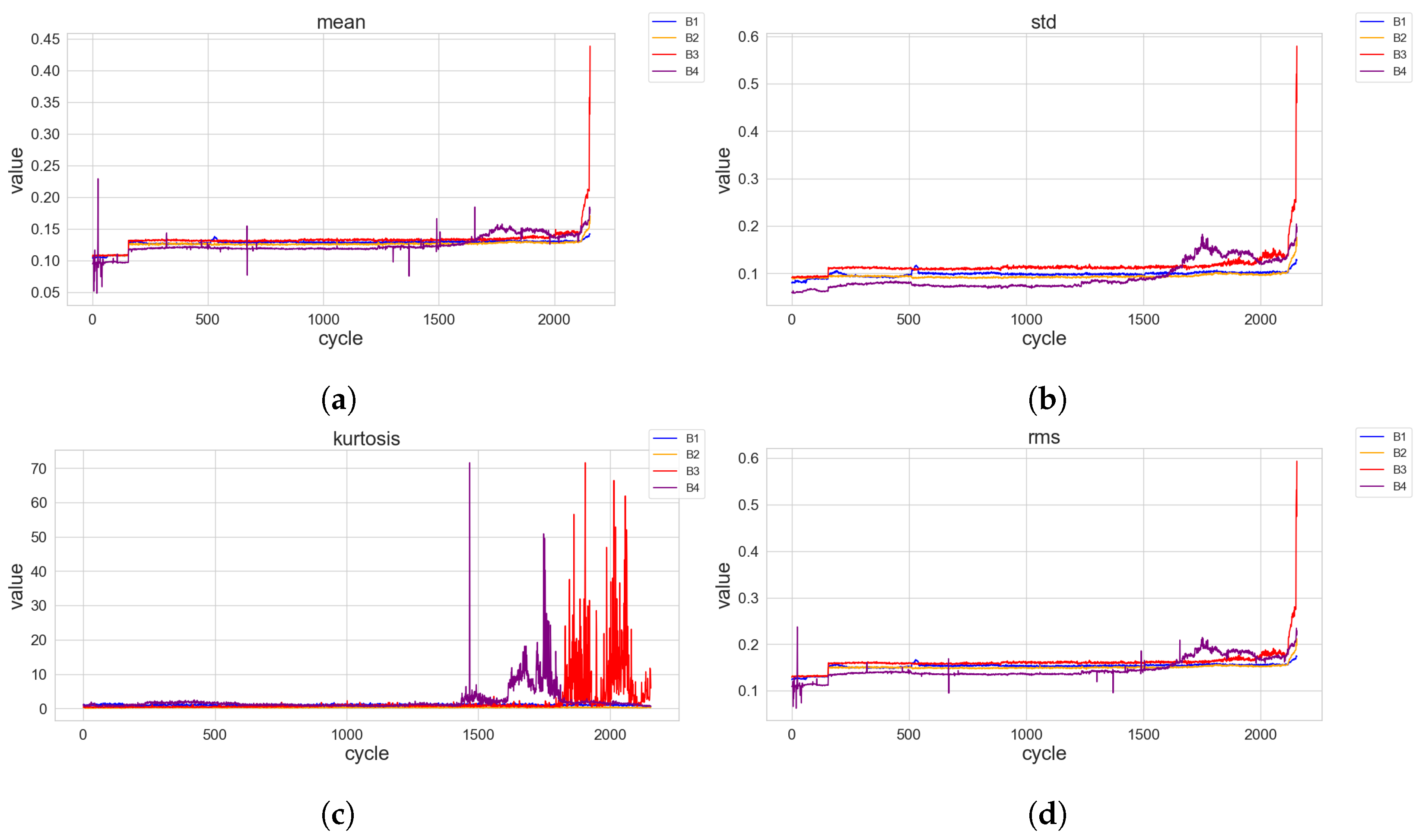
The data had been carefully cleaned to eliminate potential outliers in terms of noise, irregularities and abnormal vibration readings that might affect the accuracy of the feature extraction process, as depicted in Figure 4. By employing an array of statistical and mathematical techniques, diverse range of significant features from the vibration data were computed for a more insightful knowledge. Fundamental measurements such as mean, standard deviation, kurtosis, root mean square (RMS), skewness, entropy, maximum amplitude, peak-to-peak amplitude, crest factor, clearance factor, shape factor, and impulse were involved.

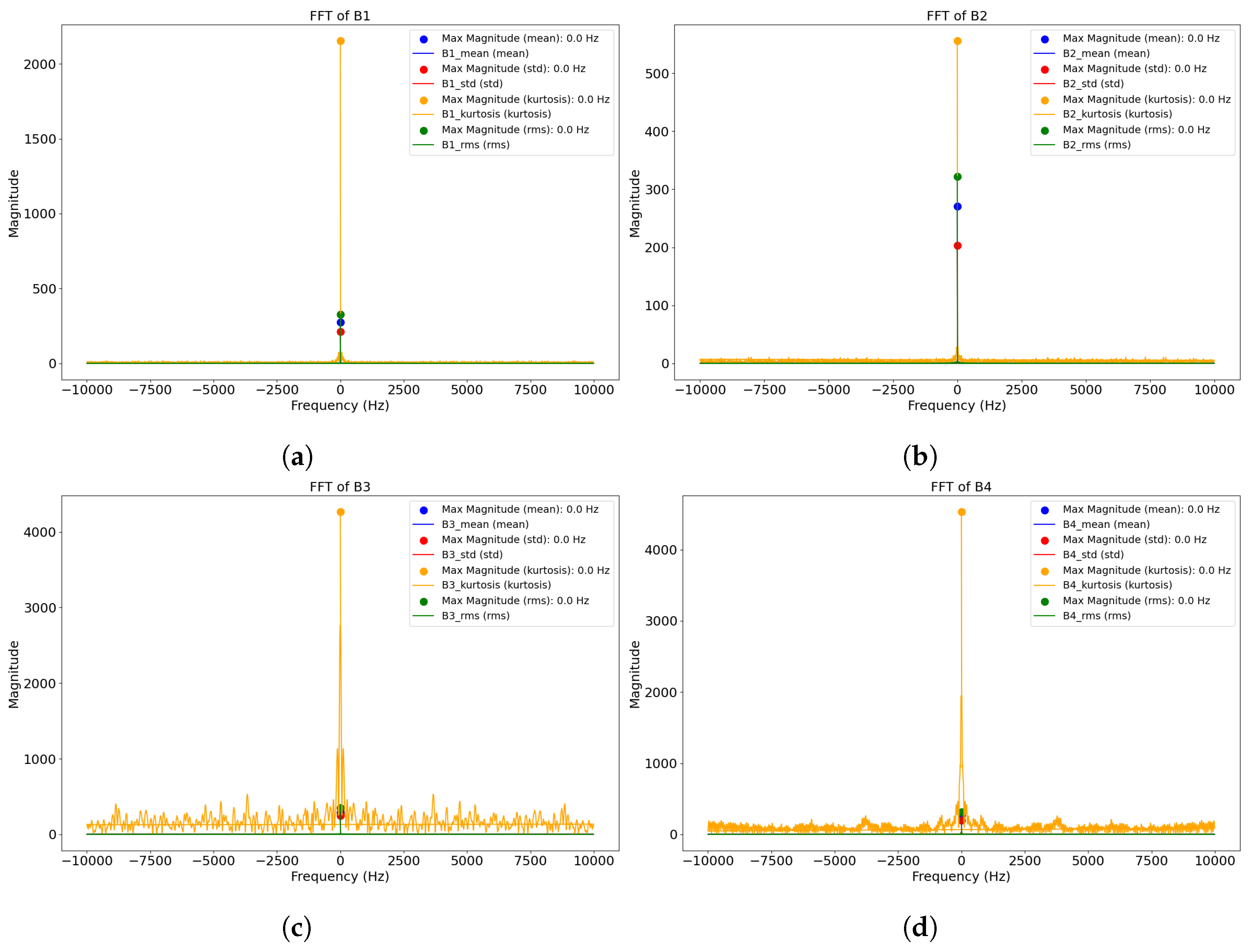
Fast Fourier Transform, Cepstrum Analysis, and Amplitude Envelope were employed to explore the periodic components and anomalies in the vibration signals are illustrated in Figure 5, Figure 6 and Figure 7. In the Fast Fourier Transform, it can be deduced that the bearings have energy distributed symmetrically around zero frequency (both positive and negative showing a projecting DC offset close to 0) with a dominant frequency component at about 290 magnitudes for mean, standard deviation, and root mean square. The Cepstrum Analysis reveals a significant Cepstrum value around data point zero, indicating an excited frequency close to 0 Hz. The Amplitude Envelope plots shared more insights into the relationship and trends between the data signals and the amplitude envelope. This suggests that there is a significant magnitude of energy around 0 Hz, indicating dominant harmonic in the signal while the presence of energy forming a “tiny cone” shape indicates the presence of noise or other low-frequency components in the signal. This perspective is based on the zoomed-out image represented in Figure 5, Figure 6 and Figure 7. We know that the fault for inner race and ball spin has been determine by [36]. However, in reality this is not the case. The kurtosis feature of the bearings has a concentrated distribution of signal levels across the frequency series with the presence of short spikes signifying distinct periodic events. Close to the zero frequency, there is the presence of widening DC component with rapid decline in energy as it moves upwards in magnitudes.

4.2. Performance Metrics and Model Evaluation

It is essential to carefully select the appropriate metrics when assessing the effectiveness of ML models on ball bearing vibration data. Considering the characteristics of the vibration data and the importance of identifying early faults in ball bearings, the following performance metrics were considered:

1.

Accuracy provides an overview of how the model’s true outcomes align with the actual outcomes. In the case where faults are uncommon, a high accuracy could be misleading. For instance, a model that predicts “no fault” can have a misleading high accuracy.

$$Accuracy=\frac{TP+TN}{TP+TN+FP+FN}$$

(1)

2.

Precision informs how many of the predicted positives are actual positives. In rotating machines, a model with high precision minimises false alarms, ensuring reliability and productivity.

$$Precision=\frac{TP}{TP+FP}$$

(2)

3.

Recall evaluates the model’s efficiency at detecting and spotting all true positive instances. It is essential for ball bearing health monitoring, because industries want to ensure as many true positives as possible are detected. Misclassifying a fault could lead to mechanical failure, leading to significant financial loss or safety risks.

$$Recall=\frac{TP}{TP+FN}$$

(3)

4.

Harmonising precision and recall, thereby providing a unified performance metric like F1, is essential. This balance aids imbalance data such as infrequent fault occurrences when comparing different models.

$$F1 score=2\times \frac{TP}{TP+FP+FN}$$

(4)

Different ML models are evaluated based on the four performance metrics mentioned above. The analysis of ML models covers the initial outcomes produced by each model and a detailed exploration of hyperparameters aimed at optimising their performance at various stages of the models evaluation process. Further details on the different ML model results are provided next.

4.2.1. Logistic Regression

After 20 test trials, the best outcome (lowest value) was an objective value of about 0.3179. This corresponds to an accuracy of 1–0.3179. The most effective setting for the C-value was about 95.28. In

Table 1. Evaluation Metrics for Logistic Regression.

Performance Metrics	Values
Accuracy	67.71%
F1 Score	59.72%
Precision	79.45%
Recall	55.41%

, the model shows accuracy of 67.71% of all predictions made by the model are correct. The harmonic mean of Precision and Recall have given a better assessment of the incorrectly classified cases than the accuracy outcome. It is essential to consider the F1 score when data classes are not evenly distributed. Of all positive predictions made by the model, about 79.45% are correct. From all actual positive cases, the model successfully detects around 55.41% of them.

4.2.2. Random Forest

A broad hyperparameter tuning was conducted to optimise the model’s performance. The primary goal was to achieve the highest accuracy and reduce inconsistences as much as possible. During the optimisation process, various sets of hyperparameters were assessed while undergoing 20 trials with each trials testing different combination of hyperparameters. The best configurations identified were: ‘n_estimators’: 967, ‘max_depth’: 10, ‘min_samples_split’: 4, ‘min_samples_leaf’: 2, ‘max_features’: ‘sqrt’}. These optimal settings attained a good accuracy rate of 84.46%, as shown in

Table 2. Evaluation Metrics for Random Forest.

Performance Metrics	Values
Accuracy	84.46%
F1 Score	83.56%
Precision	90.07%
Recall	79.71%

. This suggests that in all 85% of the instances, the RF model made true predictions. A high precision value indicates that a significant amount of the RF model’s positive predictions were correct as it accurately detected about 79.71% of all true positive cases.

4.2.3. Support Vector Machine (SVM)

A study was conducted to optimise the SVM model. The objective was to fine-tune the model’s performance by leveraging different hyperparameters. Each trial represented a unique combination of these hyperparameters, and after each test, the model’s performance was assessed. For instance, during the first trial, the model employed a linear approach with parameters such as C = 9.63, gamma = 10, coef0 = −0.28, and class_weights = None. This trial resulted in an accuracy of approximately 0.5560. After 20 trials of study, the model indicated the average cross validation score of about 0.7420. Once the model was fine-tuned, an accuracy value of 83.69% was achieved while F1 score was approximately 0.8465, depicting the model’s capability in balancing precision and recall.

Table 3. Evaluation Metrics for SVM.

Performance Metrics	Values
Accuracy	83.69%
F1 Score	84.65%
Precision	91.37%
Recall	80.94%

shows the SVM classifier made positive predictions with about 91.37% accuracy and managed to correctly detect about 80.94% of all true positive instances.

4.2.4. Extreme Gradient Boosting (XGBoost)

The non-boosted XGBoost classifier was initially employed for this application to compare with the performances of the other classifiers. The XGBoost accurately predicted about 85.01% of cases in the test dataset, which is a strong performance.

A new hyperparameter optimisation task was initiated to improve the performance of the model. This task consisted of 20 trials, with the first iteration giving the best improvement with a value of around 0.9661. The key hyperparameters tested involved a learning rate of 0.2469 and the use of 535 estimators. The model presented an overall improvement when compared to other models employed in this study. As shown in

Table 4. Evaluation Metrics for XGBoost.

Performance Metrics	Values
Accuracy	96.61%
F1 Score	97.10%
Precision	98.10%
Recall	96.17%

, the model achieved about 96.61% accuracy, which reveals the percentage of predictions made from all predictions. A harmonious balance between the accuracy of positive predictions and the fraction of positives that were captured was approximately 0.9710. The values 0.9810 and 0.9617 of precision and recall, respectively, show a high consistency of the model’s predictions. The average cross validation score on the training data is approximately 0.8516. The model learning curve is represented in Figure 8.

4.2.5. Long Short-Term Memory (LSTM)

According to literature, the LSTM, which is a type of RNN designed to handle sequence of data such as time series has been employed as a deep learning model to compare with other machine learning models in terms of performance and computational time. The LSTM model was trained for 50 epochs with both training and validation metrics recorded at the end of each epoch. The loss and accuracy on the training set started at 1.2653 and 0.5326, respectively, and by the tenth epoch, they improved to 0.8678 and 0.5977, respectively. This is an indication that the model was learning and improving its predictions on the training set over time. The validation loss and accuracy provide insight into how the model might perform on unseen data. There exist a decrease in validation loss and an increase in validation accuracy across the epochs. However, there were variations, indicating model overfitting.

To improve the training process and model convergence, amplitude scaling was also employed to transform the input data. The boosted LSTM model correctly detected about 79.30% of the instances, as shown in

Table 5. Evaluation Metrics for LSTM.

Performance Metrics	Values
Accuracy	79.30%
F1 Score	77.48%
Precision	86.83%
Recall	73.87%

. While a better value of 0.7748 F1 score was achieved over the non-boosted algorithm. This indicates a reasonable balance between the precision and recall. Precision numbers indicate that 86.83% of the instances detected as positives are true positives of the ball bearing health state. The model was able to identify about 73.87% of the true positive instances for each class. After 50 tested epochs, ‘unit’ and ‘dense_units’ values of 128 and 128 were found as the best choices, respectively. Activation was evaluated with ‘tanh’ and ‘softmax’, with ‘tanh’ being the better configuration. The Adaptive Moment Estimation (Adam) was employed to combine the Root Mean Square Propagation (RMSprop) and Momentum for a faster convergence and effectiveness of the model. The training and validation accuracy for this model is shown in Figure 9.

4.3. Computational Time Analysis

To achieve an efficient training time suitable for real-world applications, the time taken for each model’s training was used to evaluate its computational efficiency. The models were configured and optimised. The parameters of the ML models, including the number of LSTM units and dense units, were tuned to find the best configuration. The start and end times of each model training were recorded to calculate the training time for each experiment. The analysis reveals that the training time for each model varied based on the hyperparameter configurations. The training time variations are shown in

Table 6. Computational Comparison.

Classifier	Training Time (s)
Logistic Regression	0.13
Random Forest	23.91
SVM	1.12
XGBoost	0.76
LSTM	80.58

, highlighting the impact of optimising algorithm parameters on computational efficiency.

4.4. Comparative Analysis

In a data-driven industrial setting, the evaluation of model performance is of great necessity. A thorough comparative analysis of various models is often conducted to determine a well-suited process for a given task. Each of Equations (1)–(4) plays a distinct and fundamental role in the evaluation process. The comparative analysis highlights the vital role of performance metrics in assessing the effectiveness of ML models. The selection of the most appropriate model focuses on the specific objectives of the task at hand. The performance metrics comparison of different ML models under consideration is shown in

Table 7. Comparative Analysis Evaluation of Each Model.

Model Name	Hyperparameters	Accuracy	F1 Score	Precision	Recall	Training Time
Logistic	C = 95.28	67.71%	59.72%	79.45%	55.41%	0.13 s
Regression	solver-lbfgs
Random	n-estimator = 967	84.47%	83.56%	90.07%	79.71%	23.91 s
Forest	criterion = gini
SVM	C = 9.63	83.69%	84.65%	91.37%	80.94%	1.12 s
	kernel = rbf
XGBoost	n-estimator = 535	96.61%	97.10%	98.10%	96.17%	0.76 s
	max-depth = 4
LSTM	units = 128	79.30%	77.48%	86.83%	73.87%	80.58 s
	dense-units = 128

.

In the context of accuracy, XGBoost achieved an overall measure of 96.61% at a training time of 0.76 s, indicating how well the model predicted both the positive and negative categories. This reflects the research work of [52], who demonstrated the effectiveness of XGBoost in various classification tasks. In contrast, Logistic Regression recorded the lowest accuracy of 67.71% at a training time of 0.13 s. The XGBoost model recorded the highest F1 score of 97.10%, which offers a balanced metric especially in cases of imbalanced class distribution. On the other hand, Logistic Regression logged the lowest value at 59.72%. This inconsistency highlights the challenges of Logistic Regression in imbalanced datasets, as discussed by [53].

It is evident that XGBoost is not only superior in terms of performance but is also significantly efficient in terms of training times. This efficiency can be attributed to its use of parallel and distributed computing, enabling it to reach optimal solutions faster. Furthermore, XGBoost introduces randomness in its logic, making it more robust to over-fitting, and it handles missing values proficiently, resulting in accurate tree structures.

Based on these comparative analysis and observations, it is evident that XGBoost consistently out-performed other models across various key performance metrics evaluated in this study. It is also noteworthy to recognise the performance of RF, which aligns with the findings of [54], surpassing the more sophisticated LSTM exhibiting accuracy value of 79.30% at a training time of 80.58 s. This could suggest that, for this dataset, tree-based models might be more efficient than deep learning models. On the other hand, the under-performing Logistic Regression suggests its shortcomings for this dataset.

5. Conclusions

In the modern industrial systems, inefficient operations, unplanned plant downtime, and huge maintenance expenses can be caused by mechanical failures in the plant. To avoid this, conventional preventive maintenance mechanisms like time-based maintenance, oil analysis, and manual data analysis have been used previously. However, these conventional methods are time-consuming, reactive, and imprecise. Recently, advanced technologies like IoTs, big data analytics, machine learning, and cloud computing have been employed to make the modern industrial systems more efficient. In this work, we have used different machine learning models because of their high performance, ability to handle large data and adaptability to learn quickly from their experience. For comparison among different machine learning models, we have developed a framework to handle the large data from four ball bearings and extract useful features. The data preprocessing and feature extraction provided a significant insight of the data. This aided a better understanding of important patterns from vibration signals that are vital for fault detection. By comparing five distinct machine learning models, a holistic view on their computational efficiency and capability in identifying different fault categories was achieved. This comparison made it obvious how each model performed with ball bearing health status data and highlighted the effectiveness of early fault detection in modern industrial systems.

This study leverages machine learning models to evaluate various health status of four ball bearings with a total 2155 samples of vibration signals. Among the machine learning models compared, XGBoost emerges as the most favoured choice in predicting about 96.61% of all instances and 96.17% of all true positive instances at a training time of 0.76s. This study also demonstrated the superiority of XGBoost over other models under consideration when comparing the ratio of accuracy to computational time while detecting fault occurrences of the ball bearing. In the future, we would like to generate indigenous data and expand the dataset size. Larger data size would give us a better understanding of the accuracy of different ensemble algorithms and would allow us to perform an in-depth comparison with more deep learning algorithms.

References

1. Fansa Saleh, G.; Iranzo García, E.; Pérez Cueva, A.J. Comparative Analysis of Animal-Powered Waterwheels in Mediterranean Alluvial Plains: Medjerda (Tunisia) and Jucar Rivers (Spain). Land 2023, 12, 594. [Google Scholar] [CrossRef]
2. Attoui, I.; Fergani, N.; Boutasseta, N.; Oudjani, B.; Deliou, A. A new time–frequency method for identification and classification of ball bearing faults. J. Sound Vib. 2017, 397, 241–265. [Google Scholar] [CrossRef]
3. Cui, L.; Jin, Z.; Huang, J.; Wang, H. Fault Severity Classification and Size Estimation for Ball Bearings Based on Vibration Mechanism. IEEE Access 2019, 7, 56107–56116. [Google Scholar] [CrossRef]
4. Burda, E.A.; Zusman, G.V.; Kudryavtseva, I.S.; Naumenko, A.P. An Overview of Vibration Analysis Techniques for the Fault Diagnostics of Rolling Bearings in Machinery. Shock Vib. 2022, 2022, e6136231. [Google Scholar] [CrossRef]
5. de Castelbajac, C.; Ritou, M.; Laporte, S.; Furet, B. Monitoring of distributed defects on HSM spindle bearings. Appl. Acoust. 2014, 77, 159–168. [Google Scholar] [CrossRef]
6. Kulkarni, S.; Wadkar, S.B. Experimental Investigation for Distributed Defects in Ball Bearing Using Vibration Signature Analysis. Procedia Eng. 2016, 144, 781–789. [Google Scholar] [CrossRef]
7. Jadhav, P.M.; Kumbhar, S.G.; Desavale, R.G.; Patil, S.B. Distributed fault diagnosis of rotor-bearing system using dimensional analysis and experimental methods. Measurement 2020, 166, 108239. [Google Scholar] [CrossRef]
8. Hao, Y.; Zheng, C.; Wang, X.; Chen, C.; Wang, K.; Xiong, X. Damping characteristics of integral squeeze film dampers on vibration of deep groove ball bearing with localized defects. Ind. Lubr. Tribol. 2020, 73, 238–245. [Google Scholar] [CrossRef]
9. Dolenc, B.; Boškoski, P.; Juričić, Đ. Distributed bearing fault diagnosis based on vibration analysis. Mech. Syst. Signal Process. 2016, 66–67, 521–532. [Google Scholar] [CrossRef]
10. Ojaghi, M.; Sabouri, M.; Faiz, J. Analytic Model for Induction Motors Under Localized Bearing Faults. IEEE Trans. Energy Convers. 2018, 33, 617–626. [Google Scholar] [CrossRef]
11. Abu Dabous, S.; Ibrahim, F.; Feroz, S.; Alsyouf, I. Integration of failure mode, effects, and criticality analysis with multi-criteria decision-making in engineering applications: Part I—Manufacturing industry. Eng. Fail. Anal. 2021, 122, 105264. [Google Scholar] [CrossRef]
12. Tyagi, A.K.; Dananjayan, S.; Agarwal, D.; Thariq Ahmed, H.F. Blockchain—Internet of Things Applications: Opportunities and Challenges for Industry 4.0 and Society 5.0. Sensors 2023, 23, 947. [Google Scholar] [CrossRef] [PubMed]
13. Jovanovic, V.; Kuzlu, M.; Cali, U.; Utku, D.H.; Catak, F.O.; Sarp, S.; Zohrabi, N. Digital Twin in Industry 4.0 and Beyond Applications. In Digital Twin Driven Intelligent Systems and Emerging Metaverse; Springer: Singapore, 2023; pp. 155–174. [Google Scholar]
14. Aceto, G.; Persico, V.; Pescapé, A. Industry 4.0 and health: Internet of things, big data, and cloud computing for healthcare 4.0. J. Ind. Inf. Integr. 2020, 18, 100129. [Google Scholar] [CrossRef]
15. Sahal, R.; Breslin, J.G.; Ali, M.I. Big data and stream processing platforms for Industry 4.0 requirements mapping for a predictive maintenance use case. J. Manuf. Syst. 2020, 54, 138–151. [Google Scholar] [CrossRef]
16. Rai, R.; Tiwari, M.K.; Ivanov, D.; Dolgui, A. Machine learning in manufacturing and industry 4.0 applications. Int. J. Prod. Res. 2021, 59, 4773–4778. [Google Scholar] [CrossRef]
17. Dalzochio, J.; Kunst, R.; Pignaton, E.; Binotto, A.; Sanyal, S.; Favilla, J.; Barbosa, J. Machine learning and reasoning for predictive maintenance in Industry 4.0: Current status and challenges. Comput. Ind. 2020, 123, 103298. [Google Scholar] [CrossRef]
18. Huber, M.; Meier, J.; Wallimann, H. Business analytics meets artificial intelligence: Assessing the demand effects of discounts on Swiss train tickets. Transp. Res. Part B Methodol. 2022, 163, 22–39. [Google Scholar] [CrossRef]
19. Yang, Q.; Liu, Y.; Chen, T.; Tong, Y. Federated Machine Learning: Concept and Applications. ACM Trans. Intell. Syst. Technol. 2019, 10, 1–19. [Google Scholar] [CrossRef]
20. Grève, Z.D.; Bottieau, J.; Vangulick, D.; Wautier, A.; Dapoz, P.D.; Arrigo, A.; Toubeau, J.F.; Vallée, F. Machine learning techniques for improving self-consumption in renewable energy communities. Energies 2020, 13, 4892. [Google Scholar] [CrossRef]
21. Cicceri, G.; Tricomi, G.; D’Agati, L.; Longo, F.; Merlino, G.; Puliafito, A. A Deep Learning-Driven Self-Conscious Distributed Cyber-Physical System for Renewable Energy Communities. Sensors 2023, 23, 4549. [Google Scholar] [CrossRef]
22. Ciaburro, G. Machine fault detection methods based on machine learning algorithms: A review. Math. Biosci. Eng. 2022, 19, 11453–11490. [Google Scholar] [CrossRef] [PubMed]
23. Chen, T.; Sampath, V.; May, M.C.; Shan, S.; Jorg, O.J.; Aguilar Martín, J.J.; Stamer, F.; Fantoni, G.; Tosello, G.; Calaon, M. Machine Learning in Manufacturing towards Industry 4.0: From ‘For Now’ to ‘Four-Know’. Appl. Sci. 2023, 13, 1903. [Google Scholar] [CrossRef]
24. Miao, S.; Zhou, C.; AlQahtani, S.A.; Alrashoud, M.; Ghoneim, A.; Lv, Z. Applying machine learning in intelligent sewage treatment: A case study of chemical plant in sustainable cities. Sustain. Cities Soc. 2021, 72, 103009. [Google Scholar] [CrossRef]
25. Cicceri, G.; Maisano, R.; Morey, N.; Distefano, S. A novel architecture for the smart management of wastewater treatment plants. In Proceedings of the 2021 IEEE International Conference on Smart Computing (SMARTCOMP), Irvine, CA, USA, 23–27 August 2021; pp. 392–394. [Google Scholar]
26. Cicceri, G.; Maisano, R.; Morey, N.; Distefano, S. SWIMS: The Smart Wastewater Intelligent Management System. In Proceedings of the 2021 IEEE International Conference on Smart Computing (SMARTCOMP), Irvine, CA, USA, 23–27 August 2021; pp. 228–233. [Google Scholar]
27. Cicceri, G.; Scaffidi, C.; Benomar, Z.; Distefano, S.; Puliafito, A.; Tricomi, G.; Merlino, G. Smart healthy intelligent room: Headcount through air quality monitoring. In Proceedings of the 2020 IEEE International Conference on Smart Computing (SMARTCOMP), Bologna, Italy, 14–17 September 2020; pp. 320–325. [Google Scholar]
28. Alanne, K.; Sierla, S. An overview of machine learning applications for smart buildings. Sustain. Cities Soc. 2022, 76, 103445. [Google Scholar] [CrossRef]
29. Rathore, S.S.; Mishra, S.; Paswan, M.K.; Sanjay. An overview of diagnostics and prognostics of rotating machines for timely maintenance intervention. IOP Conf. Ser. Mater. Sci. Eng. 2019, 691, 012054. [Google Scholar] [CrossRef]
30. Gong, Y.; Fei, J.L.; Tang, J.; Yang, Z.G.; Han, Y.M.; Li, X. Failure analysis on abnormal wear of roller bearings in gearbox for wind turbine. Eng. Fail. Anal. 2017, 82, 26–38. [Google Scholar] [CrossRef]
31. Zhong, H.; Lv, Y.; Yuan, R.; Yang, D. Bearing fault diagnosis using transfer learning and self-attention ensemble lightweight convolutional neural network. Neurocomputing 2022, 501, 765–777. [Google Scholar] [CrossRef]
32. Alonso-González, M.; Díaz, V.G.; Pérez, B.L.; G-Bustelo, B.C.P.; Anzola, J.P. Bearing Fault Diagnosis With Envelope Analysis and Machine Learning Approaches Using CWRU Dataset. IEEE Access 2023, 11, 57796–57805. [Google Scholar] [CrossRef]
33. Abedin, T.; Koh, S.P.; Chong, T.Y.; Chen, C.P.; Tiong, S.K.; Tan, J.D.; Ali, K.; Kadirgama, K.; Benedict, F. Vibration Signal for Bearing Fault Detection using Random Forest. J. Phys. Conf. Ser. 2023, 2467, 012017. [Google Scholar] [CrossRef]
34. Nayana, B.R.; Geethanjali, P. Analysis of Statistical Time-Domain Features Effectiveness in Identification of Bearing Faults From Vibration Signal. IEEE Sens. J. 2017, 17, 5618–5625. [Google Scholar] [CrossRef]
35. Qiu, H.; Lee, J.; Lin, J.; Yu, G. Wavelet filter-based weak signature detection method and its application on rolling element bearing prognostics. J. Sound Vib. 2006, 289, 1066–1090. [Google Scholar] [CrossRef]
36. Gousseau, W.; Antoni, J.; Girardin, F.; Griffaton, J. Analysis of the Rolling Element Bearing data set of the Center for Intelligent Maintenance Systems of the University of Cincinnati. In Proceedings of the CM2016, Charenton, France, 10–12 October 2016. [Google Scholar]
37. Cardoso, D.; Ferreira, L. Application of Predictive Maintenance Concepts Using Artificial Intelligence Tools. Appl. Sci. 2021, 11, 18. [Google Scholar] [CrossRef]
38. Wang, Y.; Xia, S.T.; Tang, Q.; Wu, J.; Zhu, X. A Novel Consistent Random Forest Framework: Bernoulli Random Forests. IEEE Trans. Neural Netw. Learn. Syst. 2018, 29, 3510–3523. [Google Scholar] [CrossRef]
39. Scornet, E. Random Forests and Kernel Methods. IEEE Trans. Inf. Theory 2016, 62, 1485–1500. [Google Scholar] [CrossRef]
40. Muideen, A.A.; Lee, C.K.M.; Chan, J.; Pang, B.; Alaka, H. Broad Embedded Logistic Regression Classifier for Prediction of Air Pressure Systems Failure. Mathematics 2023, 11, 1014. [Google Scholar] [CrossRef]
41. Wang, Z.; Hong, T.; Piette, M.A. Building thermal load prediction through shallow machine learning and deep learning. Appl. Energy 2020, 263, 114683. [Google Scholar] [CrossRef]
42. Sarswatula, S.A.; Pugh, T.; Prabhu, V. Modeling Energy Consumption Using Machine Learning. Front. Manuf. Technol. 2022, 2, 855208. [Google Scholar] [CrossRef]
43. Yuan, M.; Wu, Y.; Lin, L. Fault diagnosis and remaining useful life estimation of aero engine using LSTM neural network. In Proceedings of the 2016 IEEE International Conference on Aircraft Utility Systems (AUS), Beijing, China, 10–12 October 2016; pp. 135–140. [Google Scholar] [CrossRef]
44. Ahmad, W.; Khan, S.A.; Islam, M.M.M.; Kim, J.M. A reliable technique for remaining useful life estimation of rolling element bearings using dynamic regression models. Reliab. Eng. Syst. Saf. 2019, 184, 67–76. [Google Scholar] [CrossRef]
45. Rahman, U.; Mahbub, M.U. Application of classification models on maintenance records through text mining approach in industrial environment. J. Qual. Maint. Eng. 2022, 29, 203–219. [Google Scholar] [CrossRef]
46. Aminisharifabad, M.; Yang, Q.; Wu, X. A Deep Learning-Based Reliability Model for Complex Survival Data. IEEE Trans. Reliab. 2021, 70, 73–81. [Google Scholar] [CrossRef]
47. Assi, K.J.; Nahiduzzaman, K.M.; Ratrout, N.T.; Aldosary, A.S. Mode choice behavior of high school goers: Evaluating logistic regression and MLP neural networks. Case Stud. Transp. Policy 2018, 6, 225–230. [Google Scholar] [CrossRef]
48. Su, H.; Li, X.; Yang, B.; Wen, Z. Wavelet support vector machine-based prediction model of dam deformation. Mech. Syst. Signal Process. 2018, 110, 412–427. [Google Scholar] [CrossRef]
49. Huang, X.; Shi, L.; Suykens, J.A.K. Support Vector Machine Classifier With Pinball Loss. IEEE Trans. Pattern Anal. Mach. Intell. 2014, 36, 984–997. [Google Scholar] [CrossRef] [PubMed]
50. Vos, K.; Peng, Z.; Jenkins, C.; Shahriar, M.R.; Borghesani, P.; Wang, W. Vibration-based anomaly detection using LSTM/SVM approaches. Mech. Syst. Signal Process. 2022, 169, 108752. [Google Scholar] [CrossRef]
51. Kingma, D.P.; Ba, J. Adam: A Method for Stochastic Optimization. arXiv 2017, arXiv:1412.6980. [Google Scholar]
52. Liu, J.; Cheng, H.; Liu, Q.; Wang, H.; Bu, J. Research on the Damage Diagnosis Model Algorithm of Cable-Stayed Bridges Based on Data Mining. Sustainability 2023, 15, 2347. [Google Scholar] [CrossRef]
53. Hasanin, T.; Khoshgoftaar, T.M.; Leevy, J.L.; Bauder, R.A. Severely imbalanced Big Data challenges: Investigating data sampling approaches. J. Big Data 2019, 6, 1–25. [Google Scholar] [CrossRef]
54. Li, J.; Zhu, D.; Li, C. Comparative analysis of BPNN, SVR, LSTM, Random Forest, and LSTM-SVR for conditional simulation of non-Gaussian measured fluctuating wind pressures. Mech. Syst. Signal Process. 2022, 178, 109285. [Google Scholar] [CrossRef]
Figure 1. Example of two ball bearings with distributed and localised defects. (a) A ball bearing with distributed defects; (b) A ball bearing with a localised defect.
Electronics 13 00438 g001
Figure 2. Statistical features of the vibration signals. (a) Mean of vibration signals of four ball bearings over multiple cycles; (b) Standard deviation of vibration signals of four ball bearings over multiple cycles; (c) Kurtosis of vibration signals of four ball bearings over multiple cycles; (d) Root mean square of vibration signals of four ball bearings over multiple cycles.
Electronics 13 00438 g002
Figure 3. Vibration signal intensity plot of ball bearings.
Electronics 13 00438 g003
Figure 4. Root mean square anomaly detection for four ball bearings. (a) Root mean square anomaly detection of ball bearing 1; (b) Root mean square anomaly detection of ball bearing 2; (c) Root mean square anomaly detection of ball bearing 3; (d) Root mean square anomaly detection of ball bearing 4.
Electronics 13 00438 g004
Figure 5. FFT analysis of four ball bearings vibration signals. (a) FFT analysis of ball bearing 1 vibration signals; (b) FFT analysis of ball bearing 2 vibration signals; (c) FFT analysis of ball bearing 3 vibration signals; (d) FFT analysis of ball bearing 4 vibration signals.
Electronics 13 00438 g005
Figure 6. Cepstrum analysis of four ball bearings vibration signals. (a) Cepstrum analysis of ball bearing 1 vibration signals; (b) Cepstrum analysis of ball bearing 2 vibration signals; (c) Cepstrum analysis of ball bearing 3 vibration signals; (d) Cepstrum analysis of ball bearing 4 vibration signals.
Electronics 13 00438 g006
Figure 7. Amplitude envelope analysis of four ball bearings vibration signals. (a) Amplitude envelope analysis of ball bearing 1 vibration signals; (b) Amplitude envelope analysis of ball bearing 2 vibration signals; (c) Amplitude envelope analysis of ball bearing 3 vibration signals; (d) Amplitude envelope analysis of ball bearing 4 vibration signals.
Electronics 13 00438 g007
Figure 8. XGBoost Learning Curve.
Electronics 13 00438 g008
Figure 9. Boosted LSTM Training and Validation Accuracy.
Electronics 13 00438 g009