Abstract
The Controller Area Network with Flexible Data-Rate (CAN-FD) bus is the predominant in-vehicle network protocol, responsible for transmitting crucial application semantic signals. Due to the absence of security measures, CAN-FD is vulnerable to numerous cyber threats, particularly those altering its authentic physical values. This paper introduces Physical Semantics-Enhanced Anomaly Detection (PSEAD) for CAN-FD networks. Our framework effectively extracts and standardizes the genuine physical meaning features present in the message data fields. The implementation involves a Long Short-Term Memory (LSTM) network augmented with a self-attention mechanism, thereby enabling the unsupervised capture of temporal information within high-dimensional data. Consequently, this approach fully exploits contextual information within the physical meaning features. In contrast to the non-physical semantics-aware whole frame combination detection method, our approach is more adept at harnessing the physical significance inherent in each segment of the message. This enhancement results in improved accuracy and interpretability of anomaly detection. Experimental results demonstrate that our method achieves a mere 0.64% misclassification rate for challenging-to-detect replay attacks and zero misclassifications for DoS, fuzzing, and spoofing attacks. The accuracy has been enhanced by over 4% in comparison to existing methods that rely on byte-level data field characterization at the data link layer.
1. Introduction
With the progression of information technology and the rise of the Internet of Things (IoT), intelligent connected vehicles (ICVs) have emerged as the forefront of automobile evolution. ICVs represent a next-generation breed of vehicles, outfitted with cutting-edge chips and sensors, seamlessly integrated with the Internet, and endowed with sophisticated environmental perception and advanced intelligent control systems. As vehicle interfaces proliferate and the frequency of information exchange between automotive systems and the external environment intensifies, the vulnerability of the automobile network to hacker intrusions significantly escalates. The in-vehicle Controller Area Network with Flexible Data-Rate (CAN-FD) network plays a pivotal role in facilitating real-time data exchange among multiple sensors, actuators, and ECUs situated within critical subsystems. This network is responsible for transmitting crucial physical information, such as vehicle speed, brake pressure, and the operational status of each subsystem. Vehicle manufacturers segment this data into distinct fields within the CAN-FD payload in accordance with application layer requirements. Consequently, a single CAN-FD data frame can encapsulate multiple physical attributes.
Potential security vulnerabilities in ICVs enable attackers to breach the CAN-FD network, gaining access to essential ECUs for the purpose of reading and writing through external interfaces, including physical connections (e.g., OBD II and cellular interfaces), short-range wireless connections (e.g., Bluetooth and Wi-Fi), and long-range wireless connections (e.g., over-the-air updates and GPS), as illustrated in Figure 1. Such compromise could impact specific services within the vehicle, such as the powertrain and body/chassis server. Given that CAN-FD messages encapsulate a substantial amount of information with tangible physical significance, this information is integral for actuator control. Moreover, due to the absence of robust security mechanisms, CAN-FD networks remain susceptible to a range of attacks, including denial-of-service (DoS) attacks [1], fuzzing attacks [2,3], replay attacks [4,5], and spoofing attacks [6]. These attacks involve injecting attack messages to manipulate their authentic physical meaning. In Figure 1, the first 16 bits of the message with ID 0x304 have been tampered with. Its physical meaning is linked to the speed of the vehicle and, in accordance with the communication matrix definition, can be translated into a speed signal value. The last frame with ID 0x304 in the message corresponds to a vehicle speed of 5.76 m/s. However, the tampered message now corresponds to a vehicle speed of 22.76 m/s, introducing a potential risk of loss of speed control and posing a grave threat to vehicle safety. To ensure the stability and safety of vehicle operations, it is imperative to detect anomalies within the CAN-FD network, particularly focusing on any irregularities in the physical characteristics associated with each field in the CAN-FD message. This aspect is fundamental to maintaining the normal functionality of vehicle operations.
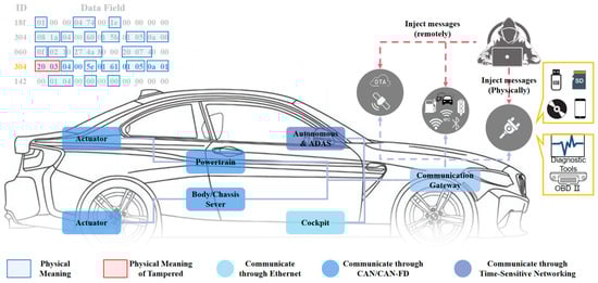
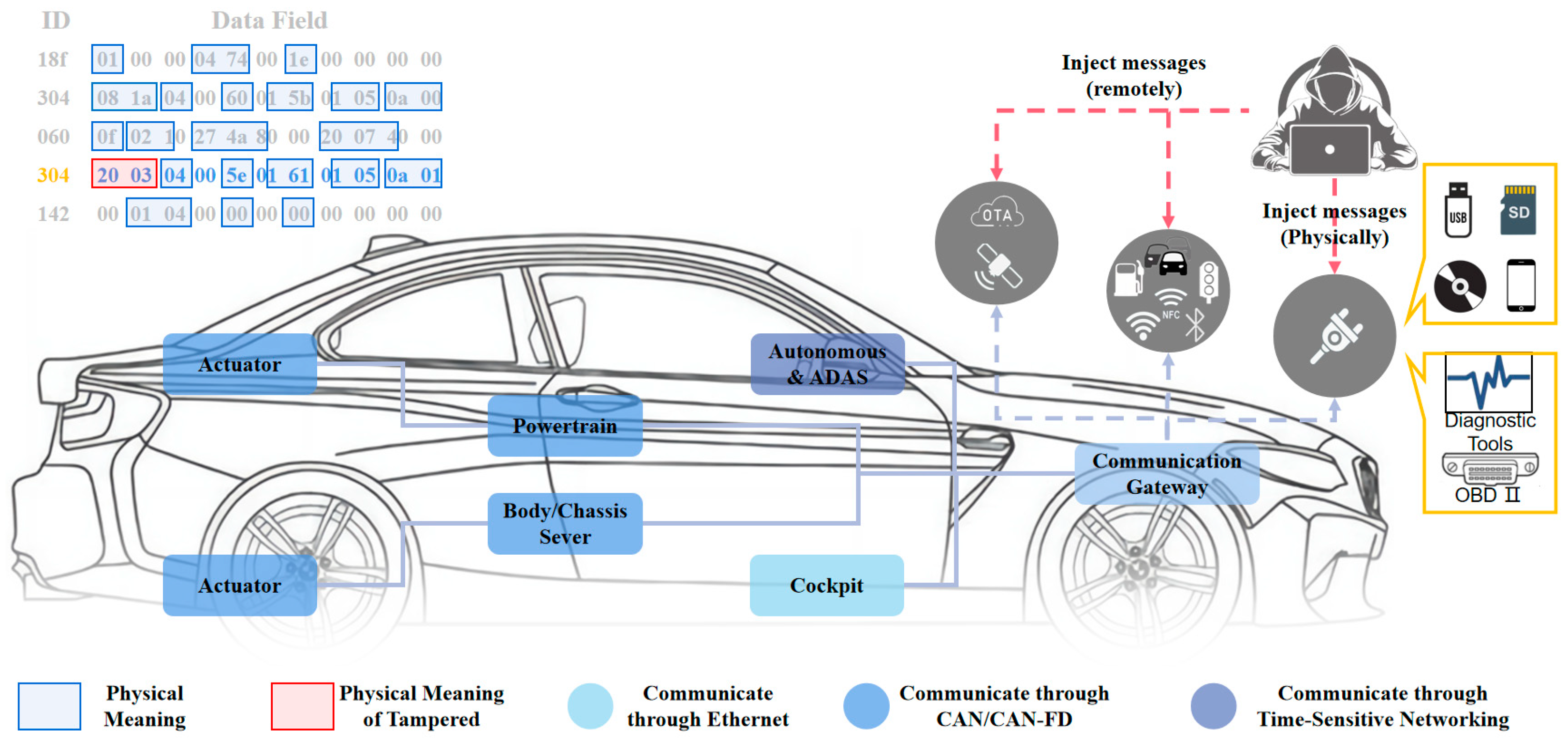
Figure 1.
In-vehicle network architecture and attack surface: The CAN/CAN-FD bus functions as the primary network application in both the powertrain and body/chassis domains within in-vehicle network architectures, exposing attack surfaces to potential threats, including near-physical contact, short-range wireless, and long-range wireless attacks.
Numerous studies have applied cryptographic algorithms, such as digital signatures, encryption, and message authentication codes, to improve message security in both CAN-FD and its foundational version, CAN. Farag [7] employs synchronized key generators across all nodes to dynamically alter the symmetric key, facilitating the encryption of the 8-byte payload data of a CAN message. This algorithm ensures the uniqueness of the encrypted message at any given time, rendering it effective in preventing replay attacks. Jo et al. [8] propose the MAuth-CAN authentication protocol to counter masquerade attacks on the CAN bus. Xie et al. [9] enhance security by incorporating message authentication codes into CAN-FD messages, achieved by promptly discarding most sequences to establish a lower bound for the on-board application and employing a generous interval from the lower bound to the deadline. Subsequently, they introduced the two-pointer moving rule to dynamically adjust the message authentication code size of each CAN-FD message, ensuring real-time performance [10]. However, the communication overhead associated with these techniques is generally high, posing challenges for their deployment in demanding real-time CAN bus networks.
In recent years, numerous intrusion detection algorithms have been proposed for CAN buses, categorized into periodicity-based and data-domain-based methods based on their detection scope and foundation. Periodicity-based methods leverage the regularity of CAN messages to identify potential anomalous behaviors within the CAN bus. Electronic Control Units (ECUs) typically generate CAN messages at specific frequencies, and deviations in message transmission frequency [11,12] or arrival interval time [13,14] can signal potential anomalies introduced by external attackers injecting messages. Normal, attack-free CAN messages exhibit standard or stable entropy, leading some researchers to propose entropy-based methods for anomaly detection in CAN [15,16]. External attacks on the CAN bus can induce abnormal changes in the physical attributes of the ECU, prompting the utilization of clock drift [17,18], clock skew [19], or voltage [20,21,22] of the ECU for anomaly detection. Olufowobi et al. [23] detect anomalies in the network based on the real-time schedulable response time of the CAN bus, while Marchetti et al. [24] construct transformation matrices using a standard CAN dataset, comparing sequences of attacked CAN message IDs to detect attacks. Yu et al. [25] establish and validate the network topology through simple random wandering-based network topology to identify external intrusion devices. Despite their effectiveness in determining the normality of message periodic properties, the aforementioned periodicity-based methods cannot identify anomalies within the data domain of the message.
Data-field-based anomaly detection methods identify anomalies by predicting the data fields of the message. Wang et al. [26] introduce an anomaly detection method based on hierarchical temporal memory (HTM) learning, wherein pre-decoded binary data streams are input into individual data sequence predictors. The output predictions are subsequently processed by an anomaly scoring mechanism. Taylor et al. [27] employ an LSTM network on CAN message data fields for prediction, utilizing prediction errors as signals for anomaly detection in the sequence. Dong et al. [28] construct a multi-observation Hidden Markov Model (HMM) based on the ID and data fields of normal CAN bus traffic. This model calculates the probability of frame existence within a defined time window and identifies anomalies based on whether the probability exceeds a threshold value. Zhang et al. [29] develop the CAN message graph, integrating statistical message sequences with message contents to construct and train Graph Neural Networks (GNNs) suitable for directed attribute graphs to predict intrusions. However, the aforementioned data-domain-based anomaly detection methods typically rely on the entire frame or individual bytes within the frame as the detection unit, resulting in a coarser detection granularity or potential segmentation of the complete physical meaning of the application. This may impede the machine’s ability to effectively learn and comprehend relevant physical features, posing challenges to improving detection accuracy.
CAN-FD presents clear advantages over CAN, including elevated data transfer rates, expanded data frames, and flexible data rates, positioning CAN-FD as a gradual replacement for conventional CAN. Current anomaly detection endeavors have concentrated on traditional CAN, with minimal consideration directed towards CAN-FD. The increased size of data frames implies that CAN-FD harbors greater physical meaning within its data fields. Given that each distinct physical meaning exhibits a unique pattern of variation, approaching the comprehensive data frame as a singular unit for detection poses a challenge in precisely delineating the normal and abnormal characteristics inherent in this heterogeneous application data. To enhance the precision and granularity of anomaly discrimination in CAN-FD networks, a shift from the data link layer to a higher network application layer is essential. Fine-grained detection for each application’s physical field within the CAN-FD data frame becomes necessary to accurately identify anomalies in the genuine physical meaning of each key feature. As a result, a Physical Semantics-Enhanced Anomaly Detection (PSEAD) method for CAN-FD data fields is proposed.
The contributions of this paper can be summarized as follows:
- Utilizing distinct physical meaning extraction rules for various ID messages, this approach extracts the genuine physical meaning features present in the data fields of CAN-FD messages. This enables the model to effectively identify abnormal variations in the vehicle’s key physical parameters. Additionally, based on the number of data types, the features associated with different CAN-FD IDs are reorganized and consolidated. The rearranged features undergo one-hot encoding and minimum-maximum scaling, significantly mitigating the dimensionality expansion introduced by one-hot encoding while preserving the numerical relationships intrinsic to the physical meanings.
- A novel CAN-FD timing prediction model, Multiple self-attention mechanisms for time-series prediction, which combines the multi-head self-attention mechanism with an LSTM network, is introduced. This model is well-suited for forecasting the physical meaning of CAN-FD messages, offering lower computational overhead and excellent real-time performance. By incorporating the multi-head self-attention mechanism, the model adeptly directs its attention to various segments within the input sequence, facilitating the acquisition of temporal feature representations across distinct hierarchical levels and granularities. This architectural choice empowers the model to holistically capture sequence information, thereby enhancing the precision of abnormal traffic detection within CAN-FD networks.
- Differing from data sources generated in simulated environments, our approach for the first time employs a dataset collected from an actual vehicle, utilizing a genuine communication protocol matrix to parse the physical meanings in CAN-FD messages. Meanwhile, attack datasets were curated by considering the mechanisms and distinctive characteristics of various attack methods. The experimental outcomes demonstrate that our method attains an accuracy improvement exceeding 4% when compared with the non-physical content-aware whole-frame combination detection method.
The remainder of this paper is structured as follows: Section 2 provides an overview of the CAN-FD message data frame composition, in-vehicle network architecture, various types of attacks, and problem definitions; Section 3 outlines the data preprocessing methods and delineates the construction of the attack dataset; Section 4 delves into the intricate design particulars of the constructed multiple self-attention mechanisms for the time-series prediction model; Section 5 focuses on the performance evaluation of the anomaly detection model; and, finally, the paper draws its conclusions in Section 6.
2. Background Information and Problem Definition
2.1. CAN-FD Background
As automotive electronic systems have grown in complexity, the traditional CAN bus protocol has faced limitations in terms of bandwidth and transmission rate. In response, CAN-FD was developed as an extension of CAN. CAN-FD offers support for data phase bit rates of up to 10 Mbps, accompanied by 64-byte payloads for messages. This extension of data fields [30] empowers CAN-FD with several advantages over CAN, including faster object pool transfer, reduced bus load usage, shorter worst-case response times, and lower jitter [31]. These characteristics render CAN-FD particularly well-suited for application scenarios where substantial data transfer is required, such as Advanced Driver Assistance Systems (ADAS) and autonomous driving. The composition of a complete CAN-FD standard data frame, as shown in Figure 2, comprises several key components:
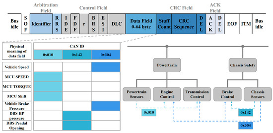
Figure 2.
CAN-FD frame structure and physical meaning of the data field.
- Start of Frame (SOF): This signals the beginning of data frame transmission.
- Arbitration Field: This field consists of the ID identifier and the RRS bit, which serve as the identification number of the receiving ECU and indicate the message’s priority. Generally, a lower ID value indicates a higher message priority.
- Control Field: This section provides control over various aspects of the data frame.
- Data Field: The core part of the message, it carries the actual data and is interpreted by the receiving ECU to discern its true physical meaning. In the case of CAN-FD, this field can hold up to 64 bytes of data.
- CRC Check Field: This field aids in detecting transmission errors. The sending node computes the CRC value and places it in this field, while the receiving node calculates the CRC using the same algorithm and compares it with the received CRC value to determine the accuracy of the message transmission.
- ACK Answer Field: All receiving nodes provide an ACK response to confirm whether the data frame was transmitted correctly.
- End of Frame (EOF): This bit marks the conclusion of the data frame.
Within the in-vehicle network, communication protocols such as CAN-FD primarily operate at the physical layer and data link layer. Automakers typically need to construct application layer protocols atop the data link layer. These three layers collaborate to facilitate the exchange of data and information among the internal components of the vehicle system connected to the CAN-FD network. The application layer protocol is responsible for defining and overseeing the data to be transmitted. For instance, it establishes the ID and the rules for the division and filling of the data domain fields. Additionally, it conveys information regarding the true physical significance of the vehicle’s speed, engine rpm, and brake pressure. To enhance cost-effectiveness, resource utilization, and network maintenance, it is often necessary to aggregate multiple signals interacting with the same ECU into a single CAN-FD frame, as illustrated in Figure 2. For instance, a message with ID 0x010 encompasses data such as shift, motor feedback speed, and torque. Both the sender and receiver of a CAN-FD message interpret the data based on a universal communication matrix. The sender of the message with ID 0x010 is the ECU responsible for powertrain, while the receivers include the ECUs associated with engine control and transmission control. The physical and data link layer communication capabilities provided by CAN-FD are then utilized to transmit this data.
2.2. Type of Attack
The broadcast nature of the CAN-FD network allows all ECUs connected to the bus to access the transmitted messages in the network. Upon receiving a CAN-FD message, each ECU arbitrates whether to accept the message based on its ID. However, the ID alone cannot authenticate the origin of a CAN-FD message without supplementary security measures. Attackers can exploit this security vulnerability to inject abnormal traffic into the CAN-FD network through various wired and wireless connections, posing a grave threat to vehicle security. Common attacks on CAN-FD networks encompass the following:
- DoS Attack: Crafted with the intent to impede authorized entities from accessing resources or to introduce delays in the operation of time-critical systems [32]. This disrupts the ability of other ECUs in the vehicle to process legitimate messages properly, potentially leading to interference, blockage, or paralysis of the CAN-FD bus. Consequently, the vehicle may become unable to function normally or carry out essential tasks.
- Fuzzing Attack: Involves the injection of randomly or semi-randomly generated data into a target system, aimed at scrutinizing the system’s response under the influence of anomalous or invalid inputs [33]. This is achieved by sending a large number of abnormal or random CAN-FD messages, which can result in erratic vehicle behavior. Symptoms may include actions such as steering wheel shaking, irregular activation of signal lights, or unexpected gear shifting [2].
- Replay Attack: Involves the recording of data from a node over a specific time interval, followed by its subsequent replay at a later point in time [34]. Legitimate CAN-FD messages are intercepted and subsequently resent to the CAN-FD bus to execute malicious operations or disrupt the vehicle’s normal operation. This can lead to the repetition of actions or inappropriate operations by the vehicle system, potentially endangering vehicle safety.
- Spoofing Attack: By transmitting counterfeit data frames to the targeted node with the aim of impersonating legitimate data or commands from an authentic source [35]. By simulating legitimate ECU communication through forged CAN-FD messages, attackers can spoof other ECUs or the vehicle control system. This can result in a loss of control over the vehicle, unintended operations, or confusion within the vehicle’s systems.
2.3. Problem Definition
The anomaly detection challenge in the CAN-FD network can be addressed by employing a network model that has acquired knowledge of typical timing variations to forecast messages. If the variance between the observed message and the predicted outcome is substantial, it can be inferred that an anomaly exists within the observed message. Assuming the training dataset is denoted as , the feature extraction process can be represented as follows:
where represents the features extracted from the training set and denotes the feature extraction function. The process of training the network model, denoted as , can be expressed as follows:
where represents the initial network model, stands for the trained network model, and symbolizes the training process. Assuming that a specific count of CAN-FD messages before the moment is represented as , where the feature , and a specific count of CAN-FD messages after the moment is denoted as , with the feature . The prediction of the message change utilizing can be expressed as follows:
where represents the anticipated feature of the CAN-FD message at a subsequent time interval, the loss value is computed by comparing with :
The threshold is defined as ; if , is considered normal, otherwise, an anomaly is detected.
3. Data Preprocessing
3.1. Data Acquisition
The initial attack-free CAN-FD dataset was gathered, comprising all CAN-FD messages transmitted on the vehicle’s CAN bus during a specific time interval. This dataset includes information such as timestamps of CAN-FD messages, IDs, data fields, and their lengths. The distribution of individual ID messages is illustrated in Figure 3a, while the variation in different CAN ID data fields is depicted in Figure 3b. To facilitate training and testing, part of the originally collected CAN-FD dataset is partitioned into the training set , while the remaining data is designated as the test set . Here, signifies a frame of message instances, and and represent message instances in the training and test sets, respectively.
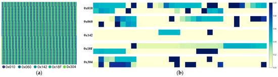
Figure 3.
Examples of the distribution of messages with varying IDs in the training set and changes in data fields: (a) various colors depict the distribution of messages with distinct IDs within the training set; (b) various colors represent alterations in the corresponding bits within the data field. Light yellow signifies that the bit remains consistently at 0, dark blue indicates that the bit remains consistently at 1, while other colors denote bits that are subject to change.
3.2. Data Augmentation
Data augmentation is a technique that expands the volume of trainable data by introducing modified versions of existing data or generating new data based on the existing dataset [36]. In our work, data augmentation was applied to the training set by altering the sliding step size of the original time-series data window and changing the sequence order of the original time-series data. Data augmentation effectively amplifies the diversity of data, intending to empower the model to grasp the inherent data domain invariants more adeptly [37]. This augmentation not only boosts the model’s generalization capabilities but also fortifies its robustness, thereby mitigating the risk of overfitting. The size of the sliding window for the input message sequence of the training set, denoted as , is represented by , and the sliding step is denoted as . Additionally, the size of the output message sequence , is represented as . In this context, the following relationships apply:
where and ( ∈ [1,2, …, ]) represent pairs of and corresponding to each other’s input and output sequences, respectively. The “ceil” function denotes the ceiling function, which rounds a number up to the nearest integer. These relationships satisfy the following conditions:
The sliding interval of the window can be controlled by employing various step sizes (where ∈ [1,2, …, ], and represents the total number of steps). In this manner, a broader range of input sequences and corresponding target output sequences can be generated based on the original data. This variation in step sizes allows for the creation of multiple input-output sequence pairs, providing a more diverse set of training data.
The training set data augmentation method is implemented in Algorithm 1, with the required initialization parameters including the training set , various sliding step sizes , the number of shuffle disruptions , the size of the sliding window , and the size of the output sequence . The algorithm proceeds as follows: It begins by generating the input sequence and the corresponding output sequence for different sliding step sizes . The input and output sequences created with different sliding steps are then randomly disrupted in correspondence, with this process being repeated times. This operation combines the input and output sequences produced in the previous step to obtain the data-enhanced input sequence and output sequence . For data augmentation of the training set, we employed a sliding window step = [1,2,3]. Subsequently, we sequentially merged the datasets generated by these three distinct sliding window steps. Following this, we subjected the merged dataset to two random disruptions. Finally, we merged the undisturbed dataset with the dataset generated by the two random disruptions, resulting in the ultimate data-augmented dataset. The aforementioned additions have been annotated in blue within the latest manuscript.
| Algorithm 1: Data augmentation | |
| Input: Training dataset , different slide step lengths , number of disruptions , sliding window size , output sequence size | |
| Output: Input sequence and output sequence after data augmentation. | |
| = empty,= empty | |
| For in do: | |
| calculate the input sequence and output sequence | |
| append →,→ | |
| End | |
| For in range do: | |
| disrupt in a random and corresponding order | |
| End | |
| For in range do: | |
| append →,→ | |
| End | |
| Return | |
3.3. Construction of the Attack Dataset
Based on the attack characteristics, this section outlines algorithms for generating attack datasets to simulate scenarios where an attacker conducts DoS, fuzzing, replay, and spoofing attacks against the CAN-FD network, as depicted in Algorithm 2. The initialization parameters needed for creating the attack dataset include the test set , the total number of selected data segments , the number of messages contained in each data segment , the range of data frames to be inserted , and the attack messages . To determine the insertion locations of the attack messages, the algorithm starts by randomly choosing non-overlapping data segments from the test set . These selected non-overlapping data segments are denoted as . Subsequently, the attack dataset is formed by randomly inserting frames of attack messages , where is a random number within the range , after each message frame within these data segments. The parameters , , , , and can be fine-tuned to align with the attack characteristics of various attack methods.
| Algorithm 2: Attack dataset generation | |||
| Input: Test dataset , total number of selected paragraphs , number of messages in each data segment , range of frames inserted , attack message | |||
| Output: Datasets subjected to attack . | |||
| = empty | |||
| select non-overlapping data segments | |||
| For in do: | |||
| append → | |||
| For in ( do: | |||
| For in range do: | |||
| append → | |||
| End | |||
| End | |||
| End | |||
| Return | |||
To create the attack dataset, the principles of different attack methods are followed, and the appropriate attack messages are injected into the normal dataset at a certain frequency. We sequentially executed denial-of-service (DoS), fuzzing, replay, and spoofing attacks on the test set. Furthermore, each of these attack messages is labeled according to the type of attack to generate the attack dataset. The attack message associated with each attack exhibits the following characteristics:
DoS attack: This type of attack is designed to disrupt the normal operation of the system by consuming the bandwidth or resources of the CAN bus. The are characterized by having an ID field of 0x000 with all zero data fields.
Fuzzy Attack: This type of attack involves searching for vulnerabilities or anomalies within the system by sending specially crafted or randomly generated CAN-FD messages. The have random ID numbers ranging from 0×000 to 0×7FF, and their data fields are filled with random data.
Replay Attack: This type of attack imitates legitimate communication by recording or intercepting a previously legitimate message and then resending it to the bus. The are identical to the previous frame messages at their insertion locations.
Spoofing Attack: In this type of attack, the vehicle’s system is spoofed by sending forged CAN-FD data frames. To generate the , the message with a specific ID is selected from the test set, and a physical feature within the message is chosen. This feature has a start bit at and an end bit at . Prior to the insertion point of the , the nearest normal message with the same ID is searched for, and the data within the range of of is modified to create the . To ensure that the generated attack message closely simulates the scenario where an attacker performs a spoofing attack, it is crucial to make the modified feature value, , sufficiently different from the original normal feature value, . Therefore, the provision:
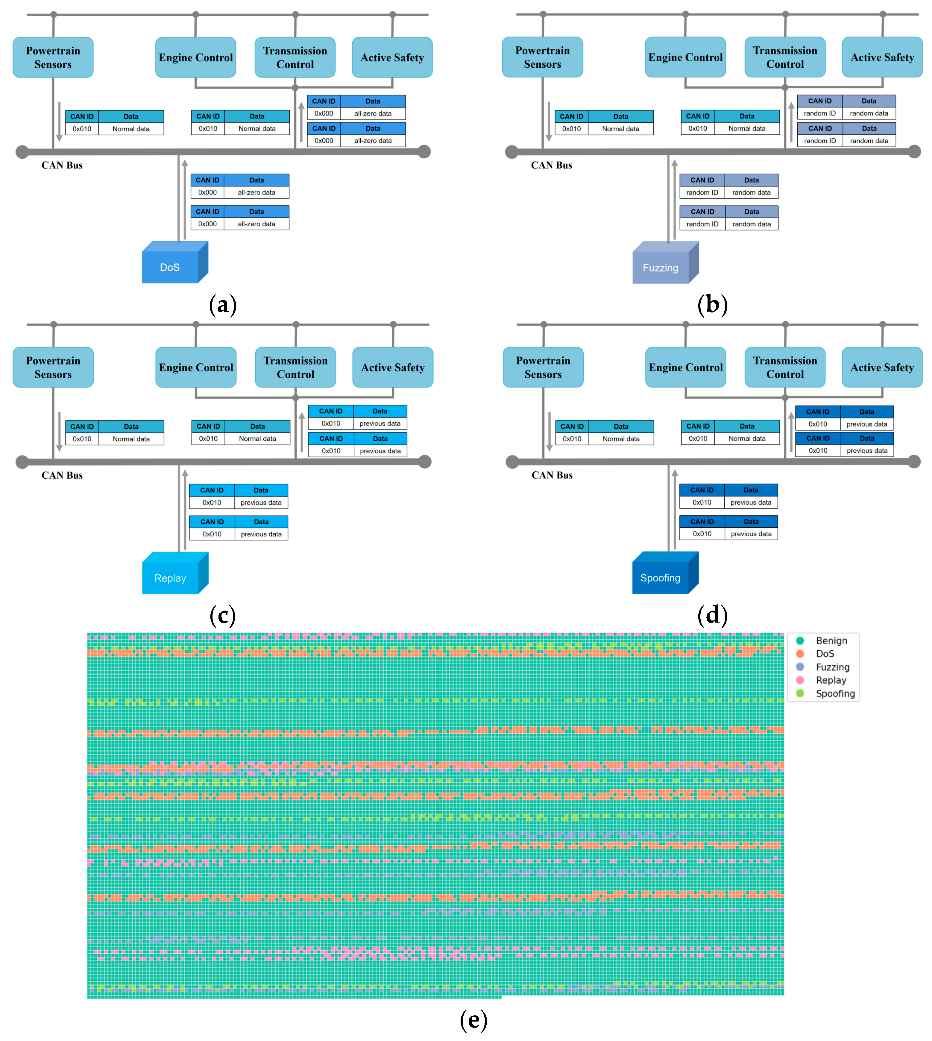
To simulate the DoS attack scenario, six data segments, each containing 100 frames of messages, were randomly selected from the original test set. Subsequently, 0–6 frames of the were randomly inserted after each frame in these segments, as depicted in Figure 4a. To simulate the fuzzy attack scenario, six segments were randomly selected from the original test set, each containing 100 frames of messages. Subsequently, 0–3 frames of the were randomly inserted after each frame in every segment, as depicted in Figure 4b. To simulate the replay attack scenario, five data segments were randomly selected from the original test set, each containing 120 frames of messages. Furthermore, 0–2 frames of the were then randomly inserted after each frame in every segment, as illustrated in Figure 4c, to simulate the replay attack scenario. To simulate a spoofing attack scenario, five data segments were randomly selected from the original test set, each containing 120 frames. Moreover, 0–2 frames of were then randomly inserted after each frame in each segment to simulate the spoofing attack scenario. For example, a can be constructed by modifying bits [20,36] in the data field of the normal message with the ID of 0x010, which corresponds to the physical quantity of motor feedback torque. This simulates the scenario of a spoofing attack, as illustrated in Figure 4d.

Figure 4.
Generation of attack dataset: (a) DoS attack, (b) fuzzing attack, (c) replay attack, (d) spoofing attack, and (e) the distribution of attack messages.
4. Physical Semantics-Enhanced Anomaly Detection
4.1. Model Framework
To detect potential anomalous messages in CAN-FD datasets, an innovative CAN-FD anomaly detection method is introduced, grounded in the genuine physical interpretations of data fields. The schematic representation of this framework is visually depicted in Figure 5, comprising four integral components: extraction and standardization of features, model training, and anomaly evaluation. Initially, feature extraction involves the extraction of authentic physical meaning features pertinent to various ID messages within the dataset, adhering to predefined extraction rules for each ID message. Subsequently, feature standardization entails the expansion of feature counts for all ID messages to align with a standardized dimension denoted as , where signifies the maximum feature count value across all ID messages. The aforementioned features are subsequently restructured, consolidated, and normalized to correspond to the number of feature types within . The same feature extraction procedure is applied to each frame, yielding the concatenated input sequence and output sequence . Model training is facilitated through the utilization of and for multiple self-attention mechanisms for time-series prediction model training. Anomaly evaluation requires the prediction of timing features using the trained multiple self-attention mechanisms for the time-series prediction model and determines whether an anomaly has occurred by comparing the difference between the predicted features and the actual features to determine whether the difference exceeds the threshold value.
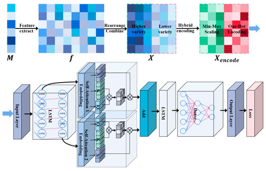
Figure 5.
The CAN-FD anomaly detection framework based on genuine physical implications.
4.2. Extraction and Standardization of Features
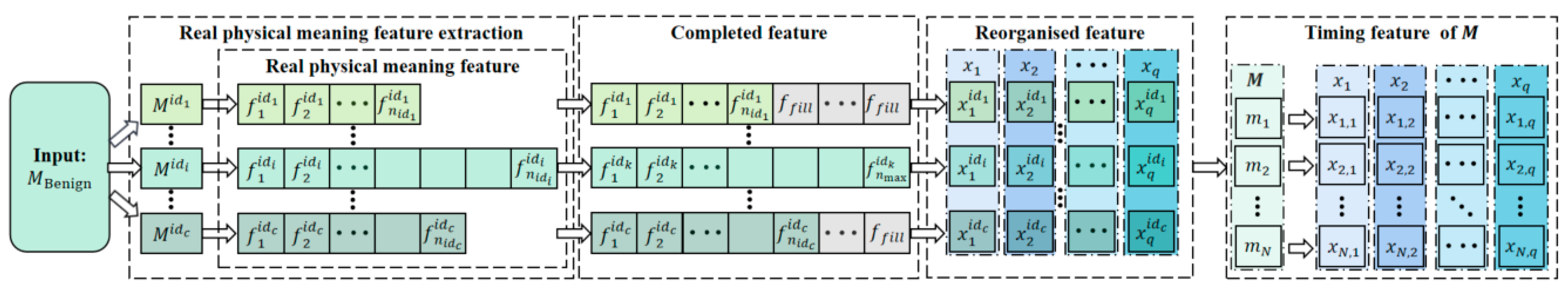
The extraction and standardization of genuine physical meaning features were conducted on the training data, as illustrated in Figure 6, and are detailed in Algorithm 3. This algorithm necessitates initialization parameters, encompassing the training set denoted as , the rule base for extracting genuine physical meaning features from various ID messages represented as , the filler feature , and the maximum number of genuine physical meaning features . For each frame of messages within the training set , the genuine physical meaning features were extracted based on their corresponding ID, following the extraction rule to preserve dataset integrity. In cases where the number of extracted features fell below , the feature count was augmented to using the . Subsequently, the extracted features were organized in descending order, taking into account the number of data types for each feature within each ID. This arrangement effectively mitigated the dimensionality inflation resulting from subsequent selective thermal encoding. These rearranged features were also standardized. Finally, eigenvalues for features with constant values were aggregated to enhance the model’s capacity to capture changing patterns in other critical features and to mitigate the risk of overfitting.
| Algorithm 3: Feature extraction and standardization | ||
| Input: Training dataset , genuine physical meaning extraction rule base , additional feature , maximum number of genuine physical meaning features | ||
| Output: Standardized features . | ||
| = empty, = empty | ||
| For in do: | ||
| If < then: | ||
| append (-)*→ | ||
| End | ||
| append → | ||
| End | ||
| For in do: | ||
| descend order by data type | ||
| standardized | ||
| End | ||
| For in do: | ||
| If unique ==1 then: | ||
| drop → | ||
| End | ||
| End | ||
| Return | ||
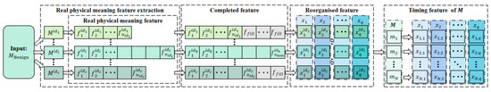
Figure 6.
The process of extracting genuine physical meaning features.
To standardize the features, a min–max scaling approach is employed. For each feature type , its minimum value and maximum value are calculated. Subsequently, the feature values within are mapped to using the following equation:
The features that are incorporated include the message IDs and their corresponding genuine physical meaning features. Features with a count of variable types not exceeding are encoded uniquely through a thermal encoding method, effectively mitigating the influence of weight bias and distance metrics. Conversely, for features with a variable type of count surpassing , their physical-value relationships are maintained to enrich the model’s comprehension of their authentic physical meaning features.
It is essential to note that, in cases where a message lacks a corresponding extraction rule in , its features will be populated with . During feature rearrangement in the test set , the order of rearrangement for each ID and the minimum and maximum for each feature type, used for standardization, remain consistent with those from the training set .
4.3. Training and Evaluation of Time-Series Prediction Models with Multiple Self-Attention Mechanisms
To obtain the input and output of the network model, features are extracted from all messages in the training set, which is denoted as . Where , indicating the -th class of features extracted from the message. Meanwhile, (j ∈ {1, 2, …, }) represents a feature value extracted from the -th frame of the message in the training set, and denotes the total number of training samples. Therefore, for , the following relationship holds:
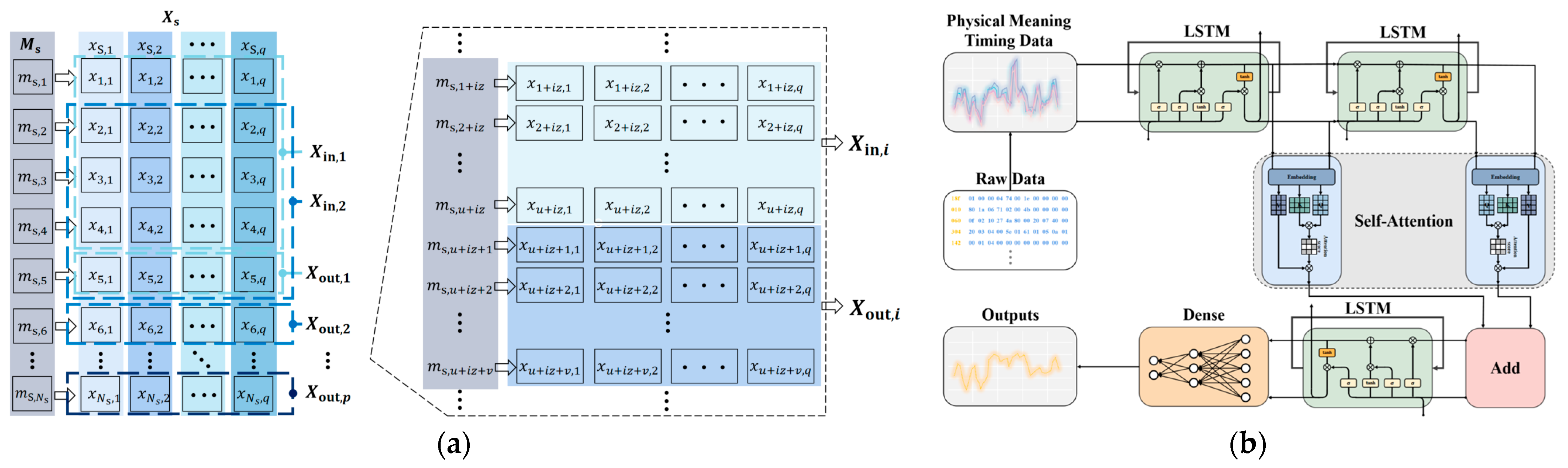
The input sequence, denoted as , and the output sequence, denoted as , are composed of features extracted from distinct sliding windows, as depicted in Figure 7a:
where and () form a paired relationship within the sequences and . In other words, when is provided as input, the anticipated output is for which and have the following relationship:

Figure 7.
The training process of the model includes: (a) model inputs and outputs; (b) multiple self-attention mechanisms for time-series prediction model architecture.
The architecture of the multiple self-attention mechanisms for time-series prediction model, as depicted in Figure 7b, incorporates a two-layer LSTM network following the input layer. This addition is aimed at enhancing the model’s ability to grasp temporal patterns and trends in the data, facilitating predictions for future time steps. Given that the cell states of the LSTM can transfer information across different time steps within the sequence, they are proficient at capturing long-term dependencies and prove effective in handling prediction tasks that demand the retention of extended historical information. LSTM’s gating mechanism enables superior management of gradient flow, mitigating the issue of gradient vanishing or explosion that traditional RNNs often encounter when dealing with lengthy sequences. The primary components of the LSTM cell architecture include an input gate , an output gate , and a forget gate . The LSTM relies on these three gates for feature selection, and their computation is as follows:
where ,, and represent the weighting matrices, ,, and are biases that are learned during the training process, are input vectors, are hidden input vectors, and signifies a sigmoid function. The process of generating candidate storage units for updating the information is as follows:
Let denote the new cell state and represent the old cell state. The process of updating the cell state is as follows:
The hidden output vector is defined as:
The forgetting gate chooses the information to retain from the old cell state , while the input gate decides the amount of information to be preserved.
In order to facilitate the modeling of associations among different positions within the sequence, capturing long-range dependencies and crucial information, a self-attention layer is introduced after the two-layer LSTM network. The core concept of the self-attention mechanism is to project each element within the sequence into a high-dimensional space and then determine element-specific weights by assessing the similarity between different elements [38]. These weights signify the degree of interconnection between the elements. This correlation empowers the model to focus on significant information at various positions, thus enhancing the processing of sequence data.
To enhance the model’s performance and bolster the network’s expressive capacity, an Add layer for residual concatenation is integrated within the self-attention layer. Subsequently, an LSTM layer is incorporated to capture and analyze temporal characteristics and patterns within the dataset. The final stage entails feature extraction and transformation through a fully connected layer, resulting in the generation of the output, denoted as .
5. Performance Evaluation and Comparative Analysis
5.1. Experiment Setup
Our experiments were conducted using Python 3.10 in the PyCharm IDE version 2023.1.2, and we implemented Keras 2.13.1 with TensorFlow 2.13.0 as the backend on a computer system equipped with an AMD Ryzen 7925HX with Radeon Graphics CPU, operating at 2.50 GHz, and 16 GB of RAM. The operating environment was Windows 11 (64-bit), and the system was equipped with an NVIDIA GeForce GTX 4060 laptop GPU.
The sliding window size for the input sequence was configured as , and the size of the output sequence was set to =1. After data preprocessing, the relevant input features and desired outputs were extracted from the training set. Subsequently, the training of the LSTM network model, combined with the attention mechanism, was carried out. The parameters of the network model were set in accordance with the specifications outlined in Table 1.

Table 1.
The configuration of model parameters.
CAN-FD datasets were procured from real vehicles, as illustrated in Figure 8. The CAN-FD transceiver, Kvaser HybridPro 2XCAN/LIN (manufactured by Kvaser, based in Brumma, Sweden), was employed to receive each CAN-FD message from the vehicle’s powertrain subnetwork interface. Subsequently, it facilitated the conversion of these messages into information, including ID, timestamp, and data fields, which were then uploaded to a PC server. On the PC side, the data fields of the CAN-FD message for each ID are correlated with the physical meaning of the characterization application through the utilization of the CAN-FD application layer protocol matrix supplied by the vehicle manufacturer. The original format of this dataset is in hexadecimal and comprises a total of 84,956 frames. Eighty percent of the messages in this dataset were allocated to the training set, with the remaining 20% reserved for the test set. The training set encompasses 67,964 frames, while the test set comprises 16,992 frames. Subsequently, various types of attack messages were introduced into the training set to create the attack dataset, and the distinct message types were appropriately labeled. Among the novel classification labels introduced in the dataset, signifies normal messages, represents DoS attack messages, characterizes fuzzy attack messages, designates replay attack messages, and denotes spoofing attack messages. The newly generated CAN-FD attack dataset comprises a total of 20,928 frames, with the distribution of attack messages illustrated in Figure 4e. Within this dataset, there are 1789 frames containing DoS attack messages, 837 frames containing fuzzing attack messages, 571 frames featuring replay attack messages, and 607 frames containing spoofing attack messages. As indicated in Table 2, the proportion of normal messages in the generated attack dataset stands at 81.71%, with DoS attack messages constituting 8.60%, fuzzing attack messages comprising 4.02%, replay attack messages accounting for 2.75%, and spoofing attack messages representing 2.92%.
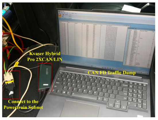
Figure 8.
Collection of authentic CAN-FD datasets from real vehicles.
Table 2.
The types and corresponding percentages of messages within the attack dataset.
These datasets were segregated in accordance with the concrete physical interpretations of data fields associated with various IDs. This partitioning facilitated the extraction of data segments with discernible physical connotations, which were subsequently transmuted into the corresponding real-world physical significance eigenvalues. The initial set of IDs encompassed 0x010, 0x142, 0x060, 0x304, and 0x18f.
The data field associated with the message ID 0x010 denoted physical quantities linked to MCU torque feedback. Message ID 0x142 was indicative of DBS state-related quantities, while message ID 0x060 encapsulated physical quantities associated with MCU drive motor feedback. Moreover, message ID 0x304 featured a data field representing the physical quantity of VCU vehicle state 2, and message ID 0x18f contained a data field representing the physical quantity associated with EPS state.
All data segments with genuine physical meanings embedded within these data fields were extracted. The values within these segments were converted to decimal format, categorized in accordance with Table 3, and assigned the corresponding feature labels in a sequential order. In order to ensure consistency, “−1” was employed to augment the number of features within each ID message, aligning them with the maximum number of features as specified in Table 3.
Table 3.
The genuine physical content encapsulated within the data fields corresponding to different IDs.
Additionally, the features within each ID message were sorted in descending order based on the nature of their values. Concurrently, they underwent normalization through min-max scaling. Finally, feature merging was carried out on features that maintained unchanged values.
5.2. Performance Evaluation
5.2.1. Evaluation Metrics
The trained model is validated through the utilization of the input features from the attack dataset in conjunction with their corresponding actual outputs. The evaluation of the model’s performance relies on a set of metrics, including TP (true positives), FP (false positives), TN (true negatives), FN (false negatives), accuracy, precision, recall, and F1 score. In order to assess the model’s performance, the trained model is loaded, and predictions are made for each element in the input features of the attack dataset. For each prediction, the mean squared loss value is computed, comparing the predicted value with its corresponding actual output.
A mean squared error threshold is established. If the mean square error loss value falls below , the prediction result aligns with our expectations, and the message is classified as normal. Conversely, if the mean square error loss value exceeds , the prediction result deviates from our expectations, and the message is deemed abnormal. The definitions of TP, FP, TN, and FN are as follows:
- TP: Represents instances where the model correctly identifies positive cases as positive.
- FP: Denotes cases where the model incorrectly identifies negative instances as positive.
- TN: Corresponds to cases where the model accurately identifies negative instances as negative.
- FN: Refers to instances where the model mistakenly identifies positive cases as negative.
Accuracy is calculated as the ratio of correctly predicted samples to the total number of samples in the model. A higher accuracy value indicates superior model performance. The accuracy can be calculated using the following formula:
Precision measures the proportion of correctly predicted positive cases among all samples that were predicted to be positive by the model. A high precision rate signifies a high degree of accuracy in the model’s positive case predictions. It can be calculated using the following formula:
Recall measures the proportion of all actual positive examples that the model correctly predicts as positive. A high recall indicates the model’s proficiency in recognizing positive examples. It is calculated as follows:
The F1 score is a metric that harmonizes precision and recall, providing a more comprehensive evaluation of the model’s performance. It is calculated as follows:
5.2.2. Experimental Verification
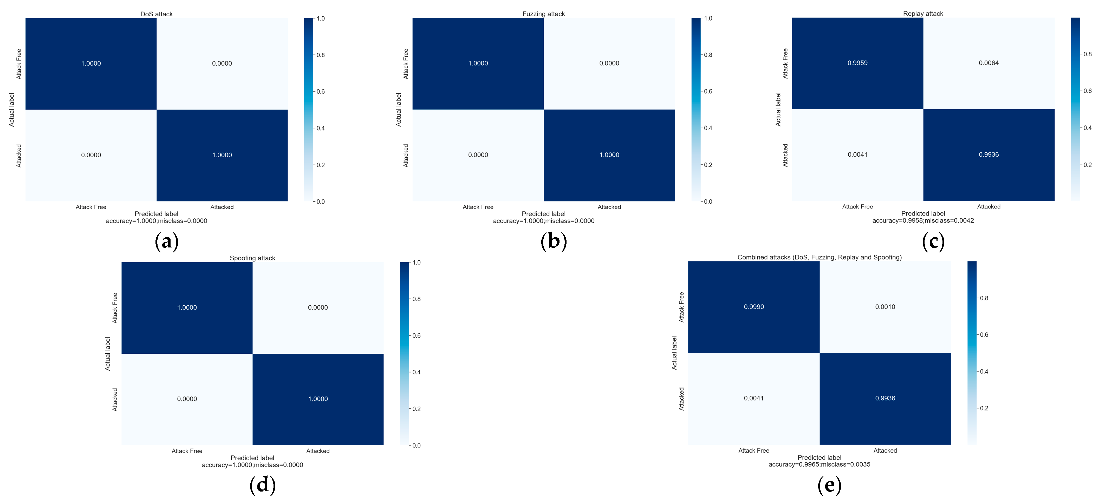
To obtain a lucid assessment of the model’s performance, it is imperative to evaluate the model’s efficacy using the aforementioned performance metrics. Figure 9 graphically depicts the relationship between the model’s predictions and the actual observations through the use of a confusion matrix, especially the model’s predictive accuracy and the rate of misclassification for normal and anomalous messages.
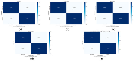
Figure 9.
The model’s performance in recognizing various types of attacks: (a) DoS attacks, (b) fuzzing attacks, (c) replay attacks, (d) spoofing attacks, and (e) hybrid attacks.
Leveraging the incorporation of authentic physical meanings in the data fields as input features and the utilization of an LSTM-based network model combined with a multi-head self-attention mechanism, the model accurately anticipates changes in the temporal characteristics of the genuine physical meanings. Table 4 illustrates the model’s accuracy in identifying different types of attacks. Under the optimal hyper-parameter configuration, the model achieves a remarkable accuracy of 99.646% in identifying anomalous messages, with an impressive F1 score of 0.99782. The recognition accuracy for DoS, fuzzing, and spoofing attacks reaches 100%, while the recognition accuracy for replay attacks, which are typically challenging to discern, remains notably high at 99.36%.
Table 4.
The model’s accuracy in recognizing a multitude of attack types.
To ascertain the significance of learning features with genuine physical meaning in messages and their impact on enhancing the model’s anomaly detection capability, it is imperative to evaluate the model’s performance when learning different input features. Reference [39] employs a deep learning-based LSTM algorithm for the detection of timing data anomalies in CAN networks. This approach demonstrates a combination of a low false alarm rate and a high detection rate, leveraging message data field byte features as input at the data link layer level. The approach in this paper, employing application layer physical semantics as input, was compared with the approach from the literature [39], which employs data link layer byte features as input, under identical training and test sets. Following the approach presented in [39], each byte (every 4 bits) within the data field was treated as a feature. In addition to this, the model’s performance was assessed when considering every two bytes (every 8 bits) as input features.
The specific outcomes are detailed in Table 5. Remarkably, models that employ input features derived from the genuine physical interpretation of data fields exhibit a 4–5% enhancement in anomaly detection accuracy when contrasted with non-physical content-aware approaches. Meanwhile, our method exhibits a misclassification rate of merely 0.412% for normal messages and a mere 0.102% for anomalous messages, whereas the method introduced in [39] demonstrates a misclassification rate exceeding 2.4% for normal messages and surpassing 12.9% for anomalous messages. This observation underscores the effectiveness of employing application-layer physical interpretations in anomaly detection, enabling the differentiation of fluctuations arising from typical operations from genuine anomalies and thereby substantially diminishing the misclassification rate for normal messages.
Table 5.
Comparison of model performance when learning different input features.
5.2.3. Ablation Study
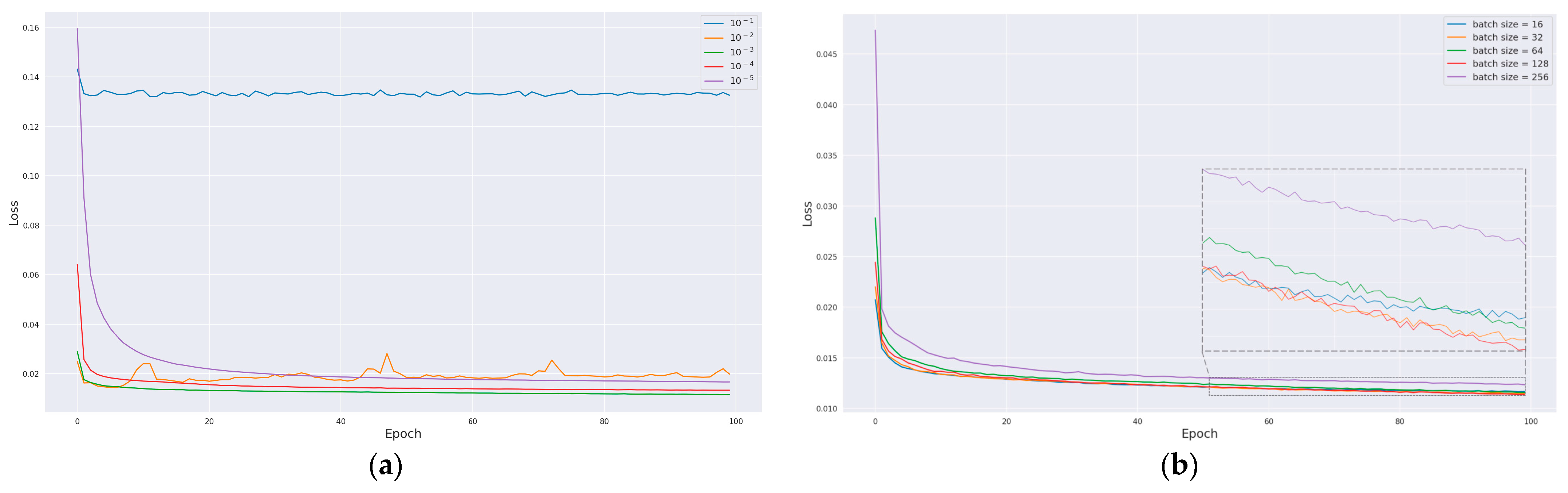
To determine the optimal learning rate, batch size, and activation function for further enhancing model performance, a comprehensive analysis was conducted. The model’s performance was assessed by comparing loss curves obtained under varying hyperparameters. Figure 10a displays the loss curves derived from training the model with different learning rates. Notably, when the learning rate is set at 0.001, the model exhibits a consistent decline in loss values throughout the training epochs, ultimately yielding the lowest loss value, thus yielding the most favorable training outcome. Subsequently, using this optimal learning rate, the impact of different batch sizes on the training performance was evaluated, as depicted in Figure 10b. The most favorable training outcome was achieved with a batch size of 128. Following this, the effect of various activation functions on model training was explored, as illustrated in Figure 10c, where it was observed that the leaky ReLU activation function demonstrated superior performance.
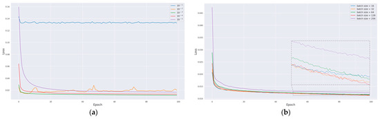
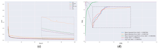
Figure 10.
Evaluation of different hyperparameters on model performance: (a) learning rate, (b) batch size, (c) activation function, and (d) ROC curves for different loss functions.
Furthermore, multiple loss functions were considered, including mean squared error, mean absolute error, mean squared logarithmic error, Huber, and log cosine error. The formula for mean squared error is provided below:
where is the number of samples, is the true value of the -th sample, and is the predicted value of the -th sample.
The formula for the mean absolute error is as follows:
The formula for the mean squared logarithmic error is expressed as follows:
The Huber loss function is defined by the following formula:
where is a non-negative constant.
The formula for the logarithmic cosine error can be expressed as follows:
The performance of the aforementioned five loss functions on the attack dataset is detailed in Table 6, while their corresponding receiver operating characteristic (ROC) curves are presented in Figure 10d. With the exception of MSLE, the area under the curve (AUC) scores of the other loss functions exhibit proximity to one another. Among these, Huber demonstrates a remarkable level of accuracy and F1 score in recognizing attack messages, second only to MSE, while concurrently achieving the highest AUC score. Consequently, it is concluded that Huber is the optimal choice for the loss function.
Table 6.
The impact of various loss functions on model performance.
To assess the effectiveness of the self-attention mechanism in enhancing the model’s ability to capture temporal features within the input data, models with variations were developed. These variations included models devoid of the attention mechanism and models employing different quantities of self-attention heads. The performance of these models is presented in Table 7. Notably, the most superior AUC score and overall performance were attained when utilizing two self-attention heads.
Table 7.
Comparison of model performance with an equal number of self-attention heads.
6. Conclusions
In this paper, an anomaly detection method for CAN-FD networks is proposed, with a focus on ascertaining the presence of abnormal network traffic by analyzing temporal changes in the genuine physical semantics within message data fields. The method commences by initially gathering CAN-FD datasets obtained from real vehicles devoid of any cyberattacks. These datasets are subsequently partitioned into a training set and a test set. The training set is further enriched through the adjustment of the sliding window step size and the introduction of sequence order disruptions. Simultaneously, the attack dataset is formulated by infusing distinct categories of attack messages into the test set, each with varying frequencies based on their specific attack attributes. Genuine physical semantic features within the message data fields are extracted and subsequently subjected to preprocessing, encompassing tasks such as padding, reordering, normalization, and consolidation. Following this, a hybrid coding methodology is applied to effectively mitigate the dimensionality inflation that typically arises from one-hot encoding. The multiple self-attention mechanisms for time-series prediction model architecture integrates the LSTM network and incorporates a multi-head self-attention mechanism to capture temporal features in the training set. The model’s hyperparameters are meticulously fine-tuned to optimize its performance. The model’s performance is then validated using the attack dataset, and its performance under varying input features is assessed. The results reveal a substantial enhancement in anomaly detection accuracy, approximately 4–5%, when utilizing the genuine physical semantics of message data fields as inputs, compared to the utilization of byte features at the data link layer level. The proposed method proves highly effective in detecting various attack types, including DoS, fuzzing, replay, and spoofing, achieving exceptional performance metrics with an F1 score of 0.99782 and an accuracy of 99.646%. Future research will delve into anomaly detection in vehicular networks, leveraging graph theory and the incorporation of the genuine physical semantics of messages.
Author Contributions
Conceptualization, R.Z. and C.L.; methodology, R.Z.; software, C.L.; validation, R.Z., C.L. and F.G.; formal analysis, C.L.; investigation, D.Z.; resources, Z.G.; data curation, L.L. and W.Y.; writing—original draft preparation, C.L.; writing—review and editing, F.G.; visualization, C.L.; supervision, R.Z.; project administration, F.G.; funding acquisition, Z.G. All authors have read and agreed to the published version of the manuscript.
Funding
This work was supported by the National Natural Science Foundation of China under Grants 52202494 and 52202495.
Data Availability Statement
The data presented in this study are available on request from the corresponding author. The data are not publicly available due to the need for confidentiality of application layer protocols for car companies.
Conflicts of Interest
The authors declare no conflict of interest.
References
- Lin, C.W.; Sangiovanni-Vincentelli, A. Cyber-security for the controller area network (CAN) communication protocol. In Proceedings of the 2012 International Conference on Cyber Security, Alexandria, VA, USA, 14–16 December 2012; pp. 1–7. [Google Scholar]
- Lee, H.; Jeong, S.H.; Kim, H.K. OTIDS: A novel intrusion detection system for in-vehicle network by using remote frame. In Proceedings of the 2017 15th Annual Conference on Privacy, Security and Trust (PST), Calgary, AB, Canada, 28–30 August 2017; pp. 57–5709. [Google Scholar]
- Islam, R.; Refat, R.U.D. Improving CAN bus security by assigning dynamic arbitration IDs. J. Transp. Secur. 2020, 13, 19–31. [Google Scholar] [CrossRef]
- Koscher, K.; Czeskis, A.; Roesner, F.; Patel, S.; Kohno, T.; Checkoway, S.; McCoy, D.; Kantor, B.; Anderson, D.; Shacham, H.; et al. Experimental security analysis of a modern automobile. In Proceedings of the 2010 IEEE Symposium on Security and Privacy, Oakland, CA, USA, 16–19 May 2010; pp. 447–462. [Google Scholar]
- Greenberg, A. Hackers remotely kill a jeep on the highway—With me in it. Wired 2015, 7, 21–22. [Google Scholar]
- Iehira, K.; Inoue, H.; Ishida, K. Spoofing attack using bus-off attacks against a specific ECU of the CAN bus. In Proceedings of the 2018 15th IEEE Annual Consumer Communications & Networking Conference (CCNC), Las Vegas, NV, USA, 12–15 January 2018; pp. 1–4. [Google Scholar]
- Farag, W.A. CANTrack: Enhancing automotive CAN bus security using intuitive encryption algorithms. In Proceedings of the 2017 7th International Conference on Modeling, Simulation, and Applied Optimization (ICMSAO), Sharjah, United Arab Emirates, 4–6 April 2017; pp. 1–5. [Google Scholar]
- Jo, H.J.; Kim, J.H.; Choi, H.Y.; Choi, W.; Lee, D.H.; Lee, I. Mauth-can: Masquerade-attack-proof authentication for in-vehicle networks. IEEE Trans. Veh. Technol. 2019, 69, 2204–2218. [Google Scholar] [CrossRef]
- Xie, G.; Yang, L.T.; Wu, W.; Zeng, K.; Xiao, X.; Li, R. Security enhancement for real-time parallel in-vehicle applications by CAN FD message authentication. IEEE Trans. Intell. Transp. Syst. 2020, 22, 5038–5049. [Google Scholar] [CrossRef]
- Xie, G.; Yang, L.T.; Liu, Y.; Luo, H.; Peng, X.; Li, R. Security enhancement for real-time independent in-vehicle CAN-FD messages in vehicular networks. IEEE Trans. Veh. Technol. 2021, 70, 5244–5253. [Google Scholar] [CrossRef]
- Moore, M.R.; Bridges, R.A.; Combs, F.L.; Starr, M.S.; Prowell, S.J. Modeling inter-signal arrival times for accurate detection of can bus signal injection attacks: A data-driven approach to in-vehicle intrusion detection. In Proceedings of the 12th Annual Conference on Cyber and Information Security Research, Oak Ridge, TN, USA, 4–6 April 2017; pp. 1–4. [Google Scholar]
- Kuwahara, T.; Baba, Y.; Kashima, H.; Kishikawa, T.; Tsurumi, J.; Haga, T.; Ujiie, Y.; Sasaki, T.; Matsushima, H. Supervised and unsupervised intrusion detection based on CAN message frequencies for in-vehicle network. J. Inf. Process. 2018, 26, 306–313. [Google Scholar] [CrossRef]
- Song, H.M.; Kim, H.R.; Kim, H.K. Intrusion detection system based on the analysis of time intervals of CAN messages for in-vehicle network. In Proceedings of the 2016 International Conference on Information Networking (ICOIN), Kota Kinabalu, Malaysia, 13–15 January 2016; pp. 63–68. [Google Scholar]
- Salem, M.; Crowley, M.; Fischmeister, S. Anomaly detection using inter-arrival curves for real-time systems. In Proceedings of the 2016 28th Euromicro Conference on Real-Time Systems (ECRTS), Toulouse, France, 5–8 July 2016; pp. 97–106. [Google Scholar]
- Müter, M.; Asaj, N. Entropy-based anomaly detection for in-vehicle networks. In Proceedings of the 2011 IEEE Intelligent Vehicles Symposium (IV), Baden-Baden, Germany, 5–9 June 2011; pp. 1110–1115. [Google Scholar]
- Marchetti, M.; Stabili, D.; Guido, A.; Colajanni, M. Evaluation of anomaly detection for in-vehicle networks through information-theoretic algorithms. In Proceedings of the 2016 IEEE 2nd International Forum on Research and Technologies for Society and Industry Leveraging a Better Tomorrow (RTSI), Bologna, Italy, 7–9 September 2016; pp. 1–6. [Google Scholar]
- Cho, K.T.; Shin, K.G. Fingerprinting electronic control units for vehicle intrusion detection. In Proceedings of the 25th USENIX Security Symposium (USENIX Security 16), Austin, TX, USA, 10–12 August 2016; pp. 911–927. [Google Scholar]
- Ji, H.; Wang, Y.; Qin, H.; Wu, X.; Yu, G. Investigating the effects of attack detection for in-vehicle networks based on clock drift of ECUs. IEEE Access 2018, 6, 49375–49384. [Google Scholar] [CrossRef]
- Halder, S.; Conti, M.; Das, S.K. COIDS: A clock offset based intrusion detection system for controller area networks. In Proceedings of the 21st International Conference on Distributed Computing and Networking, Kolkata, India, 4–7 January 2020; pp. 1–10. [Google Scholar]
- Choi, W.; Joo, K.; Jo, H.J.; Park, M.C.; Lee, D.H. VoltageIDS: Low-level communication characteristics for automotive intrusion detection system. IEEE Trans. Inf. Forensics Secur. 2018, 13, 2114–2129. [Google Scholar] [CrossRef]
- Levy, E.; Shabtai, A.; Groza, B.; Murvay, P.S.; Elovici, Y. CAN-LOC: Spoofing detection and physical intrusion localization on an in-vehicle CAN bus based on deep features of voltage signals. IEEE Trans. Inf. Forensics Secur. 2023, 18, 4800–4814. [Google Scholar] [CrossRef]
- Yin, L.; Xu, J.; Wang, C.; Wang, Q.; Zhou, F. Detecting CAN overlapped voltage attacks with an improved voltage-based in-vehicle intrusion detection system. J. Syst. Archit. 2023, 143, 102957. [Google Scholar] [CrossRef]
- Olufowobi, H.; Young, C.; Zambreno, J.; Bloom, G. Saiducant: Specification-based automotive intrusion detection using controller area network (can) timing. IEEE Trans. Veh. Technol. 2019, 69, 1484–1494. [Google Scholar] [CrossRef]
- Marchetti, M.; Stabili, D. Anomaly detection of CAN bus messages through analysis of ID sequences. In Proceedings of the 2017 IEEE Intelligent Vehicles Symposium (IV), Los Angeles, CA, USA, 11–14 June 2017; pp. 1577–1583. [Google Scholar]
- Yu, T.; Wang, X. Topology verification enabled intrusion detection for in-vehicle CAN-FD networks. IEEE Commun. Lett. 2019, 24, 227–230. [Google Scholar] [CrossRef]
- Wang, C.; Zhao, Z.; Gong, L.; Zhu, L.; Liu, Z.; Cheng, X. A distributed anomaly detection system for in-vehicle network using HTM. IEEE Access 2018, 6, 9091–9098. [Google Scholar] [CrossRef]
- Taylor, A.; Leblanc, S.; Japkowicz, N. Anomaly detection in automobile control network data with long short-term memory networks. In Proceedings of the 2016 IEEE International Conference on Data Science and Advanced Analytics (DSAA), Montreal, QC, Canada, 17–19 October 2016; pp. 130–139. [Google Scholar]
- Dong, C.; Wu, H.; Li, Q. Multiple Observation HMM-based CAN bus Intrusion Detection System for In-Vehicle Network. IEEE Access 2023, 11, 35639–35648. [Google Scholar] [CrossRef]
- Zhang, H.; Zeng, K.; Lin, S. Federated graph neural network for fast anomaly detection in controller area networks. IEEE Trans. Inf. Forensics Secur. 2023, 18, 1566–1579. [Google Scholar] [CrossRef]
- Xie, Y.; Zeng, G.; Ryo, K.; Xie, G.; Dou, Y.; Zhou, Z. An optimized design of CAN-FD for automotive cyber-physical systems. J. Syst. Archit. 2017, 81, 101–111. [Google Scholar] [CrossRef]
- Zago, G.M.; de Freitas, E.P. A quantitative performance study on CAN and CAN-FD vehicular networks. IEEE Trans. Ind. Electron. 2017, 65, 4413–4422. [Google Scholar] [CrossRef]
- Lee, Y.; Woo, S. CAN Signal Extinction-based DoS Attack on In-Vehicle Network. Secur. Commun. Netw. 2022, 2022, 9569703. [Google Scholar] [CrossRef]
- Lee, H.; Choi, K.; Chung, K.; Kim, J.; Yim, K. Fuzzing can packets into automobiles. In Proceedings of the 2015 IEEE 29th International Conference on Advanced Information Networking and Applications, Gwangju, Republic of Korea, 24–27 March 2015; pp. 817–821. [Google Scholar]
- Naha, A.; Teixeira, A.; Ahlén, A.; Dey, S. Sequential detection of replay attacks. IEEE Trans. Autom. Control 2022, 68, 1941–1948. [Google Scholar] [CrossRef]
- Yang, Y.; Duan, Z.; Tehranipoor, M. Identify a spoofing attack on an in-vehicle CAN bus based on the deep features of an ECU fingerprint signal. Smart Cities 2020, 3, 17–30. [Google Scholar] [CrossRef]
- Arantes, R.B.; Vogiatzis, G.; Faria, D.R. Learning an augmentation strategy for sparse datasets. Image Vis. Comput. 2022, 117, 104338. [Google Scholar] [CrossRef]
- Cubuk, E.D.; Zoph, B.; Mane, D.; Vasudevan, V.; Le, Q.V. Autoaugment: Learning augmentation strategies from data. In Proceedings of the IEEE/CVF Conference on Computer Vision and Pattern Recognition, Long Beach, CA, USA, 15–20 June 2019; pp. 113–123. [Google Scholar]
- Qiu, D.; Yang, B. Text summarization based on multi-head self-attention mechanism and pointer network. Complex Intell. Syst. 2022, 8, 555–567. [Google Scholar] [CrossRef]
- Qin, H.; Yan, M.; Ji, H. Application of controller area network (CAN) bus anomaly detection based on time series prediction. Veh. Commun. 2021, 27, 100291. [Google Scholar] [CrossRef]


Disclaimer/Publisher’s Note: The statements, opinions and data contained in all publications are solely those of the individual author(s) and contributor(s) and not of MDPI and/or the editor(s). MDPI and/or the editor(s) disclaim responsibility for any injury to people or property resulting from any ideas, methods, instructions or products referred to in the content. |
© 2024 by the authors. Licensee MDPI, Basel, Switzerland. This article is an open access article distributed under the terms and conditions of the Creative Commons Attribution (CC BY) license (https://creativecommons.org/licenses/by/4.0/).