Abstract
Modern electrical power networks make extensive use of high voltage direct current transmission systems based on voltage source converters due to their advantages in terms of both cost and flexibility. Moreover, incorporating a direct current link adds more complexity to the optimal power flow computation. This paper presents a new meta-heuristic technique, named self-adaptive bonobo optimizer, which is an improved version of bonobo optimizer. It aims to solve the optimal power flow for alternating current power systems and hybrid systems AC/DC, to find the optimal location of the high voltage direct current line in the network, with a view to minimize the total generation costs and the total active power transmission losses. The self-adaptive bonobo optimizer was tested on the IEEE 30-bus system, and the large-scale Algerian 114-bus electric network. The obtained results were assessed and contrasted with those previously published in the literature in order to demonstrate the effectiveness and potential of the suggested strategy.
1. Introduction
Expanding electric power networks is necessary to meet the rising demands of household and industries as well as the integration of renewable energy systems (RESs). However, this expansion leads to increased power losses, resulting in significant financial waste each year. Additionally, the effective operation of electrical networks considers various factors such as reducing fuel costs, managing network losses, minimizing environmental pollution, maintaining quality, and ensuring security and stability [1]. To ensure a reliable electricity supply, the operational state must be taken into account alongside primary objectives such as minimizing power losses, preventing voltage fluctuations, and enhancing system security. This must be achieved while adhering to various equality and inequality constraints [2]. Optimal power flow (OPF) and economic dispatch (ED) are essential aspects in power systems that require efficient coordination of generators, strategic planning, and scheduling to achieve minimization objectives [3]. The OPF problem has been a subject of study in the past for many years and is still now in the present. Despite being researched extensively since Carpentier’s work on the OPF problem 60 years ago, it continues to attract significant attention due to its challenging nature and critical significance in power system planning and operation [4]. Various modern optimization methods, such as general nonlinear optimization techniques, interior point methods, and meta-heuristic optimization methods, have been utilized to solve the OPF problem [5]. Optimizing a single or multi-objective function, while taking operational and safety constraints into consideration is the goal of OPF [6]. Conventional and modern optimization methods are the two categories of optimization algorithms. The latter are not gradient-based, multi-population algorithms that converge more quickly to the ideal or nearly ideal solution. Modern optimization algorithms can be classified into three types: artificial intelligence-based optimization algorithms (AI), meta-heuristic optimization algorithms (MAs), and combinations of two or more modern optimization techniques [7]. In recent decades, a number of meta-heuristic optimization techniques were developed and successfully applied to improve the OPF solution of various contemporary power systems [8]. For instance, one can point out the Jaya optimization technique [9], a new algorithm proposed and applied to solve single- and multi-objective OPF problem frameworks. The OPF problem has also been solved using the slime mould (SMA) and grasshopper optimization algorithm (GOA), which take into account three objectives: fuel cost, voltage profile enhancement, and minimization of active power loss [7]. In [10] the enhanced version of the equilibrium optimizer (EO) called (EEO) was used for the optimal power flow computation in a power system. This problem has also been solved using a hybridization algorithm of arithmetic optimization and Aquila optimizer [11].
The majority of countries use high-voltage alternating current (HVAC) technology in conjunction with electric power components and major alternative energy sources [12]. However, the HVAC systems are not recommended for connecting to remote renewable power plants or bulk networks due to shortcomings caused by increased power losses, additional expenses, and elevated reactive power compensation requirements [13]. Power electronic converters are increasingly used in DC microgrids, which has led to more flexible control strategies but higher line losses. The traditional hierarchical control algorithm was proposed and used to solve the OPF problem in [14] in order to reduce these losses. In [15], power electronics and its applications are reviewed. with an emphasis on loss reduction, energy efficiency, and conditioning. It makes a distinction between unidirectional and bidirectional converters, examines battery storage systems (BSS) for grid stabilization, and talks about flexible active–reactive optimal power flow (A-R-OPF) frameworks. The high voltage direct current (HVDC) transmission technology, based on voltage source converters (VSCs), has become an appealing option. It has outstanding features for controlling the AC system voltage by appropriately managing reactive power injection and absorption. Regardless of the DC transferring power, the VSC scheme can govern, respectively, real and reactive power throughout its station at the same time [16,17]. Therefore, there have been several studies conducted for this integration. In [18] a sequential algorithm for assessing load flow in hybridized AC-DC networks that takes into account all of their operational kinds in the steady-state model is presented. For multi-terminal VSC AC/DC systems, a linear MW-only power flow method with losses is formulated [19], while a generalized description of VSC-based HVDC systems suitable for power flow studies employing the Newton–Raphson method is found in [20]. In order to manage VSCs-HVDC in power systems, an AC-DC load flow process was devised, it involves uncoupling the AC network from the DC power network along with the VSC transformer stations. Nevertheless, its applicability was shown using basic test systems with 5 and 14 buses as frameworks [21]. Otherwise, coordination control considerations for these structures are complicated when integrating a connected DC system within an existing AC system [22]. This OPF problem becomes more complex compared to AC grids because of the new variables and constraints imposed on the system that must be taken into account [23]. In this case, the OPF problem in the presence of VSC-HVDC must be solved, with the use of meta-heuristic algorithms, that find the best operation of the electrical power system to minimize the total production cost and reduce power losses for the best balance of the electrical power system [24]. Although meta-heuristic solutions based on artificial intelligence have advanced, the difficult OPF problem in hybrid AC systems has received little attention [2]. In the past few years, a number of OPF algorithms have been presented for hybrid VSC-based AC/DC systems, with two key differences from their only-AC counterparts [13]:
- The optimization problem incorporates the equations for the VSC stations, DC grids, and AC/DC coupling, which are modeling components.
- Optimization variables—the VSC injections of active (P) and reactive (Q) power are control variables in the optimization problem.
In [25], the OPF problem for AC-DC grids is solved using a Newton–Raphson OPF method. The converter’s phase impedance and losses are not taken into account. In [26] the OPF problem was addressed in hybridized AC-DC systems using the DE algorithm with the intention of minimizing power losses. The simulation of marine predators was developed and used to tackle multi-objective OPF modeling in AC-DC systems [27]. A hybrid AC-DC distribution system was introduced in [28] that took into account the integration of distributed generators with soft open AC and DC. The methodology that was provided, however, was focused on reducing system power losses as a single objective. Additionally, a second-order cone program solver was used to study VSC-DC mechanisms in an optimization issue for hybrid power networks [29]. However, the particularities of the AC-DC system were disregarded in [30,31]. The DC load flow computations were disregarded in [32]. Losses were incorporated in [33], but converter limits were not, and the VSC was only partially represented. In [34] the power flow set-points were determined at the converter bus rather than the system bus, ignoring the converter losses, and the DC variables were not made available. Although this makes the calculations simpler, nevertheless, it does not follow the line of current practice.
In this paper, the self-adaptive bonobo optimizer (SABO) was used for solving the OPF in electric power networks, both with and without emerged VSC station technology, and the objective of the OPF problem was to minimize the fuel costs and transmission active power losses in system.
The main contribution of this paper can be summed up as follows:
- Implementation of the self-adaptive bonobo optimizer (SABO) was made to find the optimal location of the HVDC line in the system to optimize desired objectives
- The proposed algorithm was tested on the IEEE 30 bus and the large-scale Algerian 114-bus electric network; the simulation results were compared with several results of algorithms mentioned in other recent literature in terms of the quality and robustness of the solution.
2. VSC-HVDC Model
In this section, the AC/DC system modeling is presented, which is based on converter and DC system models that are widely recognized as state-of-the-art, as illustrated in Figure 1. As can be seen from the perspective of the AC point of common coupling (PCC), there are various components of the VSC HVDC converter station [35]:

Figure 1.
Converter station of VSC HVDC [35].
- The converter transformer
- The AC filters
- The phase reactor
- The converter.
Figure 2 shows the most general format of the converter from the AC side, so that it consists of a controllable voltage source , and it is followed by the phase reactor, which is depicted as a complex impedance . This latter is connected to a susceptance which is a component of the low pass filter. In the end, there is a transformer that is characterized by its impedance , which connects the filter bus and the AC grid. Therefore, the amount of MVA () injected into VSC from the AC system can be determined as follows:
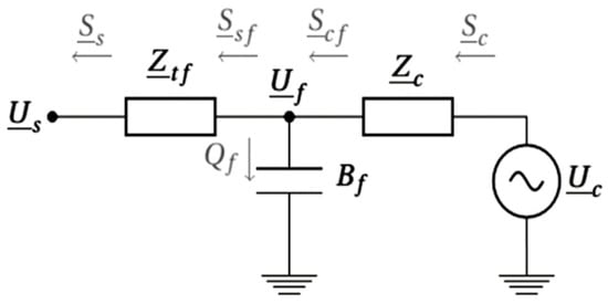
Figure 2.
Model of equivalent single-phase power flow for a converter station linked to the AC grid [35].
In which, is the AC bus voltage, and refer to the active and reactive power being injected, respectively. is the analogous injected current, and can be determined as follws:
where () represents equivalent impedance of transformer and phase reactor.
The equations representing the power flowing on the AC grid side are as follows:
The equations of active/reactive powers on the VSC side are as follows:
The formulations for the complex power flowing through the transformer on the filter side are expressed as follows:
The complex power flowing through the phase reactor side can be described as follows:
The modeling of the DC system can be depicted as a resistive network with current injections and DC voltages at various nodes [36]. The current injected into a DC node i and the power flow equation for the DC line can be expressed as follows:
where, is equal to , for the monopolar system p = 1 and for the bipolar system p = 2.
3. Formulation Problem
3.1. Objective Functions
This study formulates OPF with two objective functions, which are as below.
3.1.1. Minimization of the Total Generation Costs (TGCs)
The TGCs, expressed in USD/h, are primarily the sum of the fuel expenses for each generator. As a result, the minimization objective function of the TGCs is the first that can be represented mathematically in Equation (13) [37]:
where NG is the total number of generators, , and are the generation cost coefficients, indicates the active power output of the generator i in MW.
3.1.2. Minimization of the Total Active Power Transmission Losses (APTLs)
The APTLs , in such systems, include three sections, as in Equation (14), which contains the power losses in the AC system () explained by Equation (15), the power losses in the DC system () by Equation (16), and finally the power losses in the VSC stations () by Equation (17) [2]:
The following expression (18) indicates the current flowing through the DC link:
where V and θ are the voltage and phase angle, and NB denotes the total transmission line number, and is the conductance of the line connecting buses i and j. indicates the resistance of the DC link between buses i and j, shows the DC ampere flow along the link between buses i and j.
The factors of the losses resulting from each VSC are a, b, and c.
3.2. The Control and State Variables IN Hybrid AC/DC Network
In order for AC-DC OPF modeling to be comprehensive, it is necessary to handle novel constraint equations and additional variables specific to the DC system that are added to the known classical constraints and variables of the AC network.
3.2.1. The Control Variables
In this work, the vector of control variables u comprises both system variables AC () and DC (), respectively:
in which
where VG, PG are the voltage and the active power output of generator, T is the tap ratio of the transformer, QC is the reactive powers injected by shunt compensators, NG is the total number of generators, NT is the total number of transformers, and NC is the total number of shunt compensators , are the active and reactive power of the converter (If it is negative, it represents the power going towards the converter, i.e., the input power, and if it is positive, it represents the output power of the converter).
Moreover, since the paper wants to locate an HVDC link, the variable is used to identify the best optimal location for the link.
3.2.2. The State Variables
In this research, similarly, the set of state variables also includes state variables of AC () and DC (), respectively:
in which
and in which , are the active and reactive power generated by the slack bus, represents the reactive power of generators, is the voltage magnitude of load buses, is the apparent power flow in transmission lines, NG is the total number of generators, NL is the total load bus number, Nl is the total transmission line number, , are the active and reactive power generated by the converter in the DC slack bus, is the active power flow via DC link, and is the DC buses voltages.
3.3. Constraints
For the system to operate steadily and securely, new constraints pertaining to the operation of the HVDC link must be considered in addition to the well-known operating limitations of the AC system. Consequently, below is a summary of the constraints of the AC and DC systems [2,38].
3.3.1. The Equality Constraint
The load flow equations that need to be balanced every time are represented by the equality constraints. These constraints are defined as in Equations (25)–(27):
where, represents the generated active power, is the generated reactive power, is the active power demand, is the reactive power demand. NB is the total number of buses, and are the voltage angles at buses i and j. Correspondingly and represent the line conductance and susceptance between nodes i and j. denotes the injected MW power at bus i. is the total VSC number.
3.3.2. The Inequality Constraint
The inequality constraints are the operational bounds for the OPF AC-DC problem. There are lower and upper bounds that allow safe operation within the limits of the system. These are the standard inequality constraints that are applied to variables explained in Equations (20) and (23). The following are the lower and upper bounds that constrain these variables:
where the lowest and maximum bounds of the associated variable are indicated by the superscripts “min” and “max”.
These are inequality constraints placed on the HVDC link’s DC characteristics, which were previously specified by Equations (21) and (24). They are limited by their upper and lower boundaries, as the following:
where d is the circle’s diameter and () denotes the circle’s center relative to the PQ-capacity of the VSC.
4. Self-Adaptive Bonobo Optimizer (SABO) Algorithm
Self-adaptive bonobo optimizer (SABO) is a new algorithm first proposed in 2023, created by Amit Kumar Das Saikat Sahoo and, Dilip Kumar Pratihar. The algorithm is inspired by the social behavior and mating strategies of bonobos, with the same strategies as the BO algorithm but with more efficiency and sophistication [39]. The bonobo community depends on collective work, and on two basic processes: fission and fusion.
During the day, the bonobo community is divided into several groups of different numbers and sizes, so that each group performs specific tasks, such as searching for food or searching for safe places to live, which is what is known as the process of fission. However, with the passage of time, the bonobos reconvene with each other, and this is to perform some other tasks, such as: fighting and resisting enemies or sleeping together at night, and this is what is known as the process of fusion. As for the breeding process to create new bonobos, there are four different types of mating processes: illegal mating, mating outside the group, mating, and restricted mating, where the leader of the community and the best bonobo in the group in terms of strength and other qualities intervene in this mating process which is known as the alpha bonobo and a specific organ (called -bonobo) in the reproductive process with -bonobo.
These behaviors were modeled by the BO algorithm and the SABO algorithm proposed in this article. What distinguishes the latter is that it does not contain its own parameters as it uses memory and previous experiences in its searching mechanism, in addition to its reliance on the repulsion-based learning technique to update the parameters. Control, gives it the ability to act independently according to the needs of the situation without any manual intervention from the outside.
4.1. The SABO Works
The SABO start to initialize a randomized bonobo population of size N and evaluate its fitness, then the alpha bonobo (αbon), which is the highest ranking member of the social structure of a bonobo community, is chosen from among the other bonobos in the population according to its best fitness value; it is currently seen to be the best option solution. Alongside this process, the setting of the SABO parameters to their default values takes place. Additionally, bonobos have phase probability (pp) that alternates between positive phases (PP) and negative phases (NP), suggesting the presence of selection pressure or population diversity [40].
In SABO, the two primary regulating factors are the sharing co-efficient (β) and pp. By using repulsion-based learning, the previously described parameters can self-adjust and update over the course of several rounds. The values that are gathered throughout the search process are the only basis for this strategy. In the range of 0 to 1, both the variables pp and β have possible values. To pp or β from the present population, we provide N, the number of solutions, in each cycle.
It is expected that these parameter values will have changed from one value to another. We first create N of these parameters, each having a mean (μ) and standard deviation (σ) equal to 0.5 from a normal distribution. Changes can be made to the parameters’ lowest and maximum values. They are initially set to their highest possible value. However, in light of the demands of the search procedure, they are subsequently modified within their specified range [41].
Figure 3 and Equation (41) show the process of the repulsion technique approach to update the phase probability (pp):
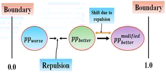
Figure 3.
The phase-probability (pp) updating through repulsion-based learning [39].
4.2. Using Different Mating Strategies to Create New Bonobos
There are four different types of bonobos mating to create new generations as mentioned above, so the mating type is determined by the phase probability (pp). (pp) has an initial value of 0.5 and is changed after each iteration.
4.2.1. Mating Strategies: Restrictive and Promiscuous
These two mating strategies are followed to create a new generation of bonobos, and they are mathematically modeled according to Equation (42):
where the -new solution is represented by the . furthermore, the solutions , , and for the current population are , , and , respectively. and are the and solutions. The third memorized population, known as badpop, and is the solution of this population. The -sharing coefficient is represented by . It is noteworthy that the four values, , and are independent and selected at random from the interval (1, N).
4.2.2. Extra-Group Mating
This mating is used if the random number is less than or equal to the probability of extra-group mating () as determined by Equations (43)–(45); this extra-group mating is utilized to update the solution:
in which the intermediate parameter is , two distinct random numbers, and were generated between the range (0, 1), the -variables of the generated solution and the -bonobo of the existing population are, respectively, and .
4.2.3. Consortship Mating
The consortship mating strategy is employed to produce a new bonobo when the value of is greater than the value of (), where is the probability of extra-group mating. This procedure is illustrated in Equations (46)–(50):
otherwise,
where,
while denotes the maximum size of group, , and dv are intermediary parameters.
4.3. Modified Boundary Handling Technique
The generated new bonobo gives a value equal to the upper limit with a chance of occurrence equal to 0.5 when it is seen to pass the upper variable limit. If not, it is updated with a probability of 0.5 using Equation (53) or (54). In a similar vein, if it is found that a new bonobo surpasses the lower variable bounds, it is made equal to its lower variable limit or the same equations are applied to make the necessary adjustments:
where is a randomly generated number in the range (0, 1).
Figure 4 shows the flowchart describing the steps involved in the SABO solution process.
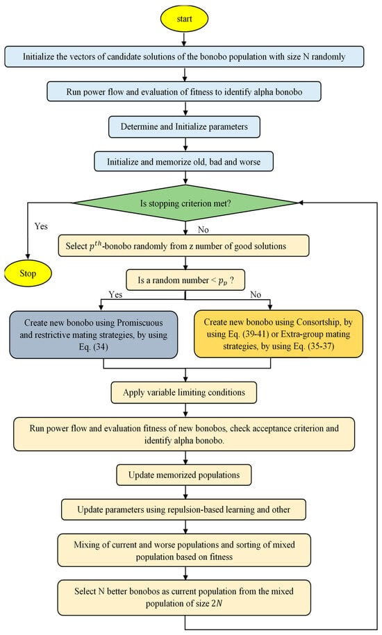
Figure 4.
Flowchart of the proposed self-adaptive bonobo optimizer (SABO).
5. Simulation Results and Discussions
The proposed algorithm SABO was applied to the IEEE 30-bus system and the large Algerian electrical test system DZ114 for minimization of two objective functions, which are the TGCs and APTLs in two different scenarios. The first is without VSC-HVDC, while the second incorporates optimizing the VSC-HVDC location. The OPF problem is addressed, by using the Matpower 4.1 and MATACDC 1.0, which are open-source, Matlab-based program. Matpower is used for calculating power flow and optimal power flow in AC systems; However, it does not have the capability to handle AC/DC systems.
The second is MATACDC; this latter uses a sequential AC/DC power flow and can be used to simulate interconnected hybrid systems AC/DC, which depend on VSC-HVDC systems [35].
The number of bonobos in the population or population size is N = 30 and the maximum number of iterations is 500 for the first system, while it is 300 iterations for the large Algerian electrical test system DZ114. All the simulations were implemented using MATLAB R2023a, and it was run on a Desktop pc with an (R) Core i3 CPU 3.0 GHz 8.0 GB RAM.
The HVDC system consists of two VSC stations and one DC branch. The parameters of the system were obtained from [13], with 345 KV for the base DC voltage converter and AC base voltage. The DC-line series resistance was 0.00334 (p.u.) for the ALG 114 BUS system [38].
5.1. IEEE 30-Bus System
The IEEE 30-bus system, consists of six generators at buses 1, 2, 5, 8, 11, and 13, 41 branches, four transformers located on lines 6–9, 4–12, 9–12, and 27–28. There are nine reactive compensators installed on buses 10, 12, 15, 17, 20, 21,23, 24, and 29. The total system load is (283.40 MW + j 126.20 Mvar), the initial power losses are (5.811 MW + j 32.417 Mvar), and the bus data and the line data are derived from [42].
5.1.1. Case-1: Minimization of Total Generation Costs (TGCs)
In this instance, the suggested method was put to the test to determine the best optimal TGCs in accordance with the production units’ best optimal power distribution as formulated in Equation (16). As shown in Table 1, it is clear that all of the optimal control variable settings fall within the permitted ranges. Furthermore, we see the best optimal TGCs without HVDC achieved by the proposed algorithm is 798.8979 (USD/h), which is the best solution obtained in comparison with various other recent methods mentioned in the literature. The algorithm took 63.8806 s to reach this solution, which is a very good time compared to the second scenario when including the HVDC line in the search, which takes 510.717 s. In addition, we can also see that when integrating the HVDC line into the network, between buses 2–5 (line 5), which is the optimal location determined by the SABO algorithm, a better result of 795.0720 (USD/h) was obtained. From Figure 5, we notice that the algorithm quickly converges towards the optimal solution in both cases, as it takes about 70 iterations. The figure also shows that the starting point for searching for the best solution is furthet away in the absence of the HVDC line compared to its presence, which means that it is able to find the optimal location within the network and was quickly identified, which allowed for a better move towards the best solution.

Table 1.
Results of optimized decision variables via SABO algorithm and various methods to minimize TGCs (IEEE 30-bus system).

Figure 5.
Comparative SABO algorithm convergence properties of TGCs (USD/h) minimization (IEEE 30-bus system).
5.1.2. Case-2: Minimization of Total Active Power Transmission Losses (APTLs)
In this case study, the minimization of the APTLs is taken into consideration. After the suggested SABO is implemented, Table 2 presents the best simulation outcome that it produced via SABO, in comparison to the best solutions obtained with various recent methods mentioned in the literature.
Table 2.
Results of optimized decision variables via SABO algorithm and various methods to minimize APTLs (IEEE 30-bus system).
As shown, the proposed SABO provides the best solution of 2.8295 in the absence of HVDC compared to the rest of the results of other algorithms. Moreover, we note that integrating the HVDC line into the optimal location between buses 2–5 as shown in Figure 6 made it possible to reach an acceptable result of 2.8483 MW, but it is not the best compared to 2.8295 MW in the case without it. This is because it includes a group of losses: power losses in AC network, converters, and DC line. Furthermore, from Table 2 we can see that the algorithm reached this solution in 64.533 s, which is very impressive considering that the second scenario takes 514.580 s when the HVDC line is included in the search; this is the same observation that was made in the case of the objective function of fuel cost. This difference is due to the additional new constraints imposed on the algorithm in the case of including an HVDC line. In addition, the network becomes more complex when hybridized, which makes reaching the optimal solution to OPF take longer.

Figure 6.
M odified IEEE-30 bus system with the optimal location of VSC-HVDC line.
When we look at these losses independently, we notice that the losses of the AC networks are 1.781 MW, which is a wonderful result compared to 2.8295 MW obtained in the case without HVDC, which means a decrease in the loss rate by 37.47%. But the losses of the converters and dc line contributed to the loss. significantly in raising it, especially the losses related to converter 0.99 MW, which represents an increase of 34.75% of the total value of the loss rate. The convergence of the algorithm is almost similar for both cases in the presence of the HVDC line and in its absence, as shown in Figure 7, so that it takes about 50 iterations to be closer to the best solution. Also, from Figure 8, we can see that the algorithm almost reaches the best solution for every run for both scenarios, except a few times when it is removed from the best solution but not by much—the worst solution was 3.1253 MW in the absence of the HVDC line while 2.9125 MW in the presence of it, which proves the flexibility and robustness of this algorithm in this case.
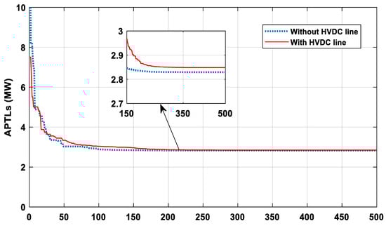
Figure 7.
Comparative SABO algorithm convergence properties of APTLs (MW) minimization (IEEE 30-bus system).
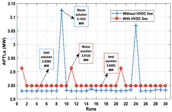
Figure 8.
APTLs solutions through the number of runs (IEEE 30-bus system).
5.2. Large Algerian Electrical Test System DZ114
To access the performance and effectiveness of the proposed approach in solving the OPF problems on large-scale real networks, this section reports the results of applying the algorithm to the large Algerian electrical test system DZ114, where the fuel cost and power losses are two single-objective functions to be studied. As usual, the results obtained by the SABO algorithm are summarized in Table 3, Table 4, Table 5 and Table 6.
Table 3.
Results of optimal settings of generators via SABO to minimize TGCs and APTLs (ALG 114-bus system).
Table 4.
Results of optimal settings of Tap ratio via SABO to minimize TGCs and APTLs (ALG 114-bus system).
Table 5.
Results of optimal settings of compensators and VSC system via SABO to minimize TGCs and APTLs (ALG 114-bus system).
Table 6.
Results of the best optimal TGCs and APTLs with best optimal location of HVDC line via SABO.
The large Algerian electrical test system DZ114 consists of 15 generators, 175 branches, and 16 transformers, with 7 reactive compensators installed and 99 load buses. The total system load is (3727 MW + j 2070 Mvar) and the initial power losses are (67.456 MW + j 265.84 Mvar) [43]. The Algerian electric system’s map is shown in Figure 9.

Figure 9.
The map of Algeria’s electricity grid [43].
5.2.1. Case-1: Minimization of Total Generation Costs (TGCs)
In this case, the objective function was to optimize the TGCs, and the results obtained are shown in Table 3, Table 4, Table 5 and Table 6. From Table 6 we can see that the result of TGCs by the proposed method in the scenario without the HVDC system is 18,928,4612 (USD/h). This optimal solution is better than other algorithm results in the literature as shown in Table 7, which confirms once again the ability of the proposed algorithm to achieve good results compared to other algorithms. Moreover, from Table 6 we can see that the integration of the HVDC line in the optimal location between bus 73–67 (Mostaghanem–Medea), which is found by the SABO algorithm, gives a better result 18,917.4349 (USD/h) compared to the result achieved in the absence of the HVDC system, i.e., 18,928.4612 (USD/h). Also, we may observe that the value of the power losses witnessed a slight decrease from 59.3861 MW without HVDC to 58.2520 MW in the case of integrated of 1.91%. From Figure 10, we see that the algorithm converges quickly towards the optimal solution faster in the absence of the HVDC line, and the starting point of the search in this case is better compared to when it is present. This is because the algorithm searches for the optimal location of the HVDC line in the second case, which takes more time due to the large size of the network. In this network, there are 175 branches, and when not counting the branches that contain transformers, there are 159 possible locations to integrate the HVDC line into, which makes the algorithm start searching for further solutions and take longer. This is one reason why the time difference between reaching the best solution in the absence of an HVDC line of 97.1380 s is much smaller than the 533.601 s when included in the research.
Table 7.
Comparison of solutions obtained via SABO with various recent methods in the literature (DZ114).
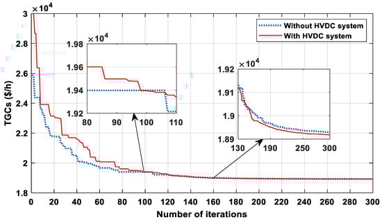
Figure 10.
Comparative SABO algorithm convergence properties of TGC minimization (ALG 114-bus system).
SABO compares favorably to numerous methods in Table 7 when it comes to minimizing TGCs. The findings of the suggested algorithm on this archive demonstrate the SABO capacity to find an optimal solution for great power systems.
5.2.2. Case-2: Minimization of Total Active Power Transmission Losses (APTLs)
In the second case, the minimization of total APTLs is taken into consideration without the HVDC system as first scenario. After running the SABO algorithm, Table 3, Table 4, Table 5 and Table 6 show the optimal results. As shown from Table 6, there is a significant reduction in power losses from 67.456 MW to 53.7 MW, which is a 20.39% decrease from the initial case. In the second scenario, which represents the integration of the HVDC line into its optimal location in the transmission network between bus 73–67 (Mostaghanem–Medea), it is noted there is a transmission loss of 53.242 MW for the AC system, 0.59 MW for the VSC stations, and 0.01 MW for the DC lines. This means that the value of the total losses of the system becomes 53.8482 MW, and a slight increase compared to the first scenario 53.6965 MW. The same observation applies to the fuel cost in this case, which rose somewhat and increased from 20,468.7419 MW in the first scenario to 20,498.3401 MW compared to the second scenario. The convergence characteristics of the proposed SABO algorithm in the presence and absence of the HVDC line are shown in Figure 11. We see that the convergence property is faster and better in the absence of the HVDC line, as it takes 80 iterations to reach the best solution compared to the case with the HVDC line, because the algorithm took approximately 120 iterations. This is due to the additional restriction imposed on the algorithm, which searches for the optimal location of the HVDC line inside this large network. Also, from Figure 12, in the absence of an HVDC line, we can see that the algorithm does not always reach the best solution in each run, as we found many results that are somewhat far from the best solution, with the worst solution in this case being 59.0988 MW. This highlights the impact of the size of the network on the proposed algorithm. Furthermore, the same observation was made in the presence of an HVDC line, as the solutions were further away than in its absence. This is because of the network’s size, as well as the additional constraints that were added to the OPF, not to mention the complexities that affect the network when it becomes hybrid AC-DC.
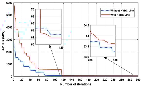
Figure 11.
Comparative SABO algorithm convergence properties of APTLs (MW) minimization (ALG 114-bus system).
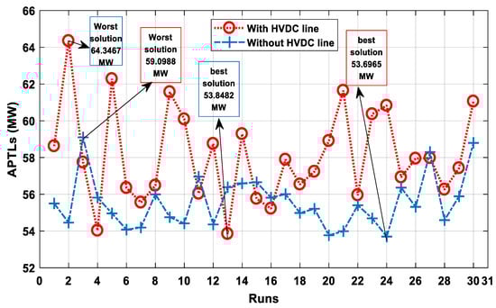
Figure 12.
APTL solutions through the number of runs (ALG 114-bus system).
6. Conclusions
This article introduced an improved version of the SABO algorithm to solve the OPF problem for AC networks and hybrid AC-DC power systems with emerged VSC stations. It aims to reduce total fuel costs and minimize active power losses in AC systems, while for hybrid AC/DC systems, it works to determine the optimal location of VSC stations to achieve the best solutions for these objectives. The SABO algorithm was effectively applied to both the IEEE 30-bus system and the real-life equivalent Algerian 114-bus network. The performance and effectiveness of SABO were verified by comparing its results with various methods documented in the literature. Using the Sabo algorithm, we achieved the best values in every case study based on the optimal control variable setting values that were reached, showing its superiority in reaching the best results. However, it was shown to be affected by the size of the network, in addition to additional limitations when the network became hybrid AC-DC, as its robustness and speed of convergence toward the solution decreased. The study also found that VSC converter losses have a minor impact on the minimized power losses in hybrid AC-DC systems. Despite having the above benefits, future work should include different scenarios of emergency situations that may affect the power networks, in order to evaluate the robustness of the algorithm under these conditions. Modeling different renewable energy sources is also one of the most important points that should be addressed in order to demonstrate the advantages of the study, as the integration of these resources highlights the necessity of hybrid AC-DC networks.
Author Contributions
H.E.A.: led the conceptualization of the study and was integral in curating and analyzing data. He conducted investigations, developed software tools, and ensured the validation and visualization of results. Additionally, he was responsible for drafting the original manuscript and contributed extensively to its review and editing. S.S.: played a crucial role in conceptualizing the research and managing data curation. He contributed to formal analysis, investigation, and methodology development. As the project administrator, he managed resources, oversaw the research process, and supervised the project. His contributions also extended to validation, visualization, and both drafting and reviewing the manuscript. A.B.: focused on formal analysis and investigation, providing key supervision and validation throughout the research process. His role also involved reviewing and editing the manuscript to ensure its accuracy and clarity. A.H.: contributed to formal analysis and investigation, playing a significant role in developing the methodology and supervising research activities. He was also involved in validation, creating visualizations, and reviewing and editing the manuscript. R.K.: managed data curation and formal analysis, and actively participated in investigations. He contributed to software development and validation of the results. His role in reviewing and editing the manuscript was also crucial to its final version. R.S.: focused on validating the results and contributed to the manuscript by reviewing and editing it to ensure accuracy and coherence. All authors have read and agreed to the published version of the manuscript.
Funding
This research received no external funding.
Data Availability Statement
Data are contained within the article.
Conflicts of Interest
The authors declare no conflict of interest.
References
- Ali, M.H.; Kamel, S.; Hassan, M.H.; Tostado-Véliz, M.; Zawbaa, H.M. An Improved Wild Horse Optimization Algorithm for Reliability Based Optimal DG Planning of Radial Distribution Networks. Energy Rep. 2022, 8, 582–604. [Google Scholar] [CrossRef]
- Sarhan, S.; Shaheen, A.M.; El-Sehiemy, R.A.; Gafar, M. Enhanced Teaching Learning-Based Algorithm for Fuel Costs and Losses Minimization in AC-DC Systems. Mathematics 2022, 10, 2337. [Google Scholar] [CrossRef]
- Khoa, T.H.; Vasant, P.M.; Singh, M.S.B.; Dieu, V.N. Swarm Based Mean-Variance Mapping Optimization for Convex and Non-Convex Economic Dispatch Problems. Memetic Comput. 2017, 9, 91–108. [Google Scholar] [CrossRef]
- Elattar, E.E.; Shaheen, A.M.; Elsayed, A.M.; El-Sehiemy, R.A. Optimal Power Flow with Emerged Technologies of Voltage Source Converter Stations in Meshed Power Systems. IEEE Access 2020, 8, 166963–166979. [Google Scholar] [CrossRef]
- Zohrizadeh, F.; Josz, C.; Jin, M.; Madani, R.; Lavaei, J.; Sojoudi, S. A Survey on Conic Relaxations of Optimal Power Flow Problem. Eur. J. Oper. Res. 2020, 287, 391–409. [Google Scholar] [CrossRef]
- Mahdad, B. Improvement Optimal Power Flow Solution Considering SVC and TCSC Controllers Using New Partitioned Ant Lion Algorithm. Electr. Eng. 2020, 102, 2655–2672. [Google Scholar] [CrossRef]
- Kouadri, R.; Musirin, I.; Slimani, L.; Bouktir, T.; Othman, M.M. Optimal Power Flow Control Variables Using Slime Mould Algorithm for Generator Fuel Cost and Loss Minimization with Voltage Profile Enhancement Solution. Int. J. Emerg. Trends Eng. Res. 2020, 8, 36–44. [Google Scholar]
- Bouchekara, H.R.E.H.; Abido, M.A.; Boucherma, M. Optimal Power Flow Using Teaching-Learning-Based Optimization Technique. Electr. Power Syst. Res. 2014, 114, 49–59. [Google Scholar] [CrossRef]
- Abd, S.; Kamel, E.S.; El, R.A.; Francisco, S.; Yu, J. Single- and Multi-Objective Optimal Power Flow Frameworks Using Jaya Optimization Technique Respectively. Neural Comput. Appl. 2019, 31, 8787–8806. [Google Scholar]
- Houssein, E.H.; Hassan, M.H.; Mahdy, M.A.; Kamel, S. Development and Application of Equilibrium Optimizer for Optimal Power Flow Calculation of Power System. Appl. Intell. 2023, 53, 7232–7253. [Google Scholar] [CrossRef]
- Ahmadipour, M.; Murtadha, M.; Bo, R.; Sadegh, M.; Mohammed, H.; Alrifaey, M. Optimal Power Flow Using a Hybridization Algorithm of Arithmetic Optimization and Aquila Optimizer. Expert Syst. Appl. 2024, 235, 121212. [Google Scholar] [CrossRef]
- Reviews, S.E.; Version, D.; Reviews, S.E. Review of VSC HVDC Connection for Offshore Wind Power Integration. Renew. Sustain. Energy Rev. 2016, 59, 1405–1414. [Google Scholar]
- Renedo, J.; Asrul, A.; Kazemtabrizi, B.; García-cerrada, A.; Rouco, L.; Zhao, Q.; García-gonzález, J.; De Investigación, I.; Iit, T.; Icai, E.; et al. Electrical Power and Energy Systems a Simplified Algorithm to Solve Optimal Power Flows in Hybrid VSC-Based. Electr. Power Energy Syst. 2019, 110, 781–794. [Google Scholar] [CrossRef]
- Ma, J.; He, F.; Zhao, Z. Line Loss Optimization Based OPF Strategy by Hierarchical Control for DC Microgrid. In Proceedings of the 2015 IEEE Energy Conversion Congress and Exposition, ECCE 2015, Montreal, QC, Canada, 20–24 September 2015; pp. 6212–6216. [Google Scholar]
- Gabash, A. Review of Battery Storage and Power Electronic Systems in Flexible A-R-OPF Frameworks. Electronics 2023, 12, 3127. [Google Scholar] [CrossRef]
- Sau-bassols, J.; Zhao, Q.; Garc, J. Optimal Power Flow Operation of an Interline Current Flow Controller in an Hybrid AC/DC Meshed Grid. Electr. Power Syst. Res. 2019, 177, 105935. [Google Scholar] [CrossRef]
- Ma, Q.; Wei, W.; Chai, W.; Mei, S. ScienceDirect Solvability Region of AC—DC Power Systems with Volatile Renewable Energy Sources. Energy Rep. 2022, 8, 1463–1472. [Google Scholar] [CrossRef]
- Beerten, J.; Belmans, R. Development of an Open Source Power Flow Software for HVDC Grids and Hybrid AC/DC Systems: MatACDC. IET Gener. Transm. Distrib. 2015, 9, 966–974. [Google Scholar] [CrossRef]
- Fernández-Pérez, J.-C.; Cerezo, F.M.E.; Rodríguez, L.R. Linear Power Flow Algorithm with Losses for Multi-Terminal VSC AC/DC Power Systems. IEEE Trans. Power Syst. 2021, 37, 1739–1749. [Google Scholar] [CrossRef]
- Karami, E.; Gharehpetian, G.B.; Mohammadpour, H.; Khalilinia, A.; Bali, A. Generalised Representation of Multi-Terminal VSC-HVDC Systems for AC—DC Power Flow Studies. IET Energy Syst. Integr. 2020, 2, 50–58. [Google Scholar] [CrossRef]
- E-hawary, M.E.; Ibrahim, S.T. A New Approach to AC-DC Load Flow Analysis. Electr. Power Syst. Res. 1995, 33, 193–200. [Google Scholar] [CrossRef]
- Feng, W.; Member, S.; Tuan, L.A.; Tjernberg, L.B.; Member, S.; Mannikoff, A.; Bergman, A.; Member, S. A New Approach for Bene Fi t Evaluation of Multiterminal VSC—HVDC Using A Proposed Mixed AC/DC Optimal Power Flow. IEEE Trans. Power Deliv. 2014, 29, 432–443. [Google Scholar] [CrossRef]
- Yang, Z.; Member, S.; Zhong, H.; Bose, A.; Fellow, L. Optimal Power Flow in AC–DC Grids with Discrete Control Devices. IEEE Trans. Power Syst. 2017, 33, 8950. [Google Scholar] [CrossRef]
- Using, H.; Lion, A. Optimal Power Flow Solution for Wind Integrated Power in Presence of VSC- Optimal Power Flow Solution for Wind Integrated Power in Presence of VSC-HVDC Using Ant Lion Optimization. Indones. J. Electr. Eng. Comput. Sci. 2018, 12, 625–633. [Google Scholar]
- Pizano-martinez, A.; Fuerte-esquivel, C.R.; Acha, E.; Member, S. Modeling of VSC-Based HVDC Systems for a Newton-Raphson OPF Algorithm. IEEE Trans. Power Syst. 2007, 22, 1794–1803. [Google Scholar] [CrossRef]
- Algorithms, G. Networks for Grid Integration of Offshore Wind Farms Using. Energies 2013, 6, 1–26. [Google Scholar]
- Elsayed, A.M.; Shaheen, A.M.; Alharthi, M.M. Adequate Operation of Hybrid AC / MT-HVDC Power Systems Using an Improved Multi-Objective Marine Predators Optimizer. IEEE Access 2021, 51065–51087. [Google Scholar] [CrossRef]
- Point, S.O. Minimization of Network Power Losses in the AC-DC Hybrid Distribution Network through Network Reconfiguration Using Soft Open Point. Electronics 2021, 10, 326. [Google Scholar] [CrossRef]
- Flow, P.; Grids, V.A.; Baradar, M.; Member, S.; Hesamzadeh, M.R. Second-Order Cone Programming for Optimal. Math. Program. 2003, 95, 3–51. [Google Scholar]
- Ac, H.; Power, D.C.; Hotz, M.; Member, S.; Utschick, W.; Member, S. Hynet: An Optimal Power Flow Framework For hybrid AC/DC power systems. IEEE Trans. Power Syst. 2019, 35, 1036–1047. [Google Scholar]
- Maulik, A.; Das, D. Optimal Power Dispatch Considering Load and Renewable Generation Uncertainties in an AC—DC Hybrid Microgrid. IET Gener. Transm. Distrib. 2019, 13, 1164–1176. [Google Scholar] [CrossRef]
- Lotfjou, A.; Fu, Y.; Shahidehpour, M. Hybrid AC / DC Transmission Expansion Planning. IEEE Trans. Power Deliv. 2012, 27, 1620–1628. [Google Scholar] [CrossRef]
- Zhao, M.; Chen, Z.; Blaabjerg, F. Load Flow Analysis for Variable Speed Offshore Wind Farms. IET Renew. Power Gener. 2009, 3, 120–132. [Google Scholar] [CrossRef]
- Gengyin, L.; Ming, Z.; Member, S.; Jie, H.; Guaagkai, L.; Haifeng, L. Power Flow Calculation of Power Systems Incorporating VSC-HVDC. In Proceedings of the 2004 International Conference on Power System Technology, Singapore, 21–24 November 2004; pp. 21–24. [Google Scholar]
- Beerten, J.; Cole, S.; Belmans, R. Generalized Steady-State VSC MTDC Model for Sequential AC/DC Power Flow Algorithms. IEEE Trans. Power Syst. 2012, 27, 821–829. [Google Scholar] [CrossRef]
- Beerten, J. MatACDC 1.0 User’s Manual. Dep. Electr. Eng. Univ. Leuven 2012, 1–36. [Google Scholar]
- Bouchekara, H.R.E.H.; Chaib, A.E.; Abido, M.A.; El-Sehiemy, R.A. Optimal Power Flow Using an Improved Colliding Bodies Optimization Algorithm. Appl. Soft Comput. J. 2016, 42, 119–131. [Google Scholar] [CrossRef]
- Sayah, S. Modified Differential Evolution Approach for Practical Optimal Reactive Power Dispatch of Hybrid AC−DC Power Systems. Appl. Soft Comput. J. 2018, 73, 591–606. [Google Scholar] [CrossRef]
- Kumar, A.; Saikat, D.; Dilip, S.; Pratihar, K. An Improved Design of Knee Orthosis Using Self–Adaptive Bonobo Optimizer (SaBO). J. Intell. Robot. Syst. 2023, 107, 8. [Google Scholar]
- Das, A.K. A New Bonobo Optimizer (BO) for Realparameter Optimization. In Proceedings of the IEEE Region 10 Symposium (TENSYMP), Kolkata, India, 7–9 June 2019. [Google Scholar]
- Farh, H.M.H.; Al-shamma, A.A.; Al-shaalan, A.M.; Alkuhayli, A. Technical and Economic Evaluation for Off-Grid Hybrid Renewable Energy System Using Novel Bonobo Optimizer. Sustainability 2022, 14, 1533. [Google Scholar] [CrossRef]
- Alsac, O.; Stott, B. Optimal Load Flow with Steady-State Security. IEEE Trans. Power Appar. Syst. 1974, PAS-93, 745–751. [Google Scholar] [CrossRef]
- Ben oualid Medani, K.; Sayah, S.; Bekrar, A. Whale Optimization Algorithm Based Optimal Reactive Power Dispatch: A Case Study of the Algerian Power System. Electr. Power Syst. Res. 2018, 163, 696–705. [Google Scholar] [CrossRef]
- Herbadji, O.; Slimani, L.; Bouktir, T. Optimal Power Flow with Four Conflicting Objective Functions Using Multiobjective Ant Lion Algorithm: A Case Study of the Algerian Electrical Network. Iran. J. Electr. Electron. Eng. 2019, 15, 94–113. [Google Scholar]
- Slimani, L.; Bouktir, T. Optimal Power Flow Solution of the Algerian Electrical Network Using Differential Evolution Algorithm. TELKOMNIKA Indones. J. Electr. Eng. 2012, 10, 199–210. [Google Scholar]
- Mahdad, B.; Srairi, K. Solving Practical Economic Dispatch Using Hybrid GA-DE-PS Method. Int. J. Syst. Assur. Eng. Manag. 2014, 5, 391–398. [Google Scholar] [CrossRef]
- Kouadri, R.; Musirin, I.; Slimani, L.; Bouktir, T. OPF for Large Scale Power System Using Ant Lion Optimization: A Case Study of the Algerian Electrical Network. IAES Int. J. Artif. Intell. 2020, 9, 252–260. [Google Scholar] [CrossRef]
Disclaimer/Publisher’s Note: The statements, opinions and data contained in all publications are solely those of the individual author(s) and contributor(s) and not of MDPI and/or the editor(s). MDPI and/or the editor(s) disclaim responsibility for any injury to people or property resulting from any ideas, methods, instructions or products referred to in the content. |
© 2024 by the authors. Licensee MDPI, Basel, Switzerland. This article is an open access article distributed under the terms and conditions of the Creative Commons Attribution (CC BY) license (https://creativecommons.org/licenses/by/4.0/).