Multi-Objective Combinatorial Optimization Algorithm Based on Asynchronous Advantage Actor–Critic and Graph Transformer Networks

Abstract

Multi-objective combinatorial optimization problems (MOCOPs) are designed to identify solution sets that optimally balance multiple competing objectives. Addressing the challenges inherent in applying deep reinforcement learning (DRL) to solve MOCOPs, such as model non-convergence, lengthy training periods, and insufficient diversity of solutions, this study introduces a novel multi-objective combinatorial optimization algorithm based on DRL. The proposed algorithm employs a uniform weight decomposition method to simplify complex multi-objective scenarios into single-objective problems and uses asynchronous advantage actor–critic (A3C) instead of conventional REINFORCE methods for model training. This approach effectively reduces variance and prevents the entrapment in local optima. Furthermore, the algorithm incorporates an architecture based on graph transformer networks (GTNs), which extends to edge feature representations, thus accurately capturing the topological features of graph structures and the latent inter-node relationships. By integrating a weight vector layer at the encoding stage, the algorithm can flexibly manage issues involving arbitrary weights. Experimental evaluations on the bi-objective traveling salesman problem demonstrate that this algorithm significantly outperforms recent similar efforts in terms of training efficiency and solution diversity.

1. Introduction

MOCOPs [1,2] are centered on the identification of optimal combinations of decision variables within discrete decision spaces. Unlike single-objective optimization, where a singular objective is pursued, MOCOPs are characterized by the necessity to balance multiple, often conflicting, objectives [3]. This inherent complexity has spurred the development of more precise and efficient methods, aimed at achieving comprehensive optimization across various criteria [4].

Current strategies for solving MOCOPs are divided into two types: exact and approximate algorithms [5,6]. Exact algorithms seek precise solutions but often face practical limitations in large-scale combinatorial problems [7] due to the extensive computational demands [8] and complex constraints [9], thereby hindering their application in engineering practice. In contrast, approximate algorithms, including heuristic and metaheuristic methods, offer a higher efficiency and flexibility for large-scale problems [10]. Heuristic algorithms simplify the solving process based on specific rules [11,12], quickly finding feasible solutions, and are particularly suited for large problems due to their rapid solution time. However, these may not guarantee optimal results and sometimes make assessing the solution quality challenging as they primarily focus on rapidly finding feasible solutions rather than systematically exploring all possibilities [13]. Metaheuristic algorithms [14], such as the multi-objective evolutionary algorithm based on decomposition (MOEA/D) [15], non-dominated sorting genetic algorithm II (NSGA-II) [16], and multi-objective genetic local search (MOGLS) [17], simulate natural evolutionary [18,19] or physical processes to explore the solution space, providing superior global search capabilities over simple heuristic methods. These algorithms typically do not depend on the problem’s specific structure, thus offering better generalizability. However, they require manual adjustments for specific problems and may need redesigning as problem scales change, often leading to local optima and extended search durations.

In recent years, DRL [20,21,22,23] has emerged as an ideal approach for addressing MOCOPs, as a result of its ability to efficiently manage high-dimensional and complex decision spaces [24] and adapt to dynamic environments and requirements [25]. This method utilizes an end-to-end solving framework [26], leveraging encoder–decoder [27,28] architectures that incrementally build solutions by adding nodes and edges. While DRL-based multi-objective combinatorial optimization algorithms [29] have made significant advancements, they continue to face challenges in balancing model complexity [30], training efficiency, and solution diversity [31,32]. Consequently, developing deep neural networks that can effectively extract features from large-scale problems, and designing efficient training strategies under memory constraints has become essential.

Given these considerations, this paper introduces a novel multi-objective combinatorial optimization algorithm based on DRL, named MOA3C-GTN. The key contributions include the implementation of the A3C [33] training mode, which updates multiple agents asynchronously using an advantage function, thereby enhancing environmental adaptability, accelerating convergence [34], and improving solution quality and diversity. Additionally, the algorithm leverages the characteristics of MOCOPs by allowing each node to serve as a potential starting point for the policy network, enabling the construction of diverse trajectories and effectively avoiding local optima, thus enhancing performance and reliability. Furthermore, the design of the GTNs [35,36,37] incorporates features for edge characteristics and objective weights, effectively utilizing additional information from edges to generate solutions for any given weight vector in MOCOPs.

The structure of the paper is as follows: Section 2 reviews the related work, Section 3 introduces the MOA3C-GTN algorithm, Section 4 compares MOA3C-GTN with recent algorithms, and Section 5 concludes the paper and outlines future research directions.

2. Related Work

This section outlines the definition of MOCOPs and the current state of research on multi-objective combinatorial optimization algorithms based on DRL, and introduces the DRL-MOA algorithm.

2.1. Multi-Objective Combinatorial Optimization Problems

The mathematical model for a general MOCOP can be described as follows:

$$\left\{\begin{array}{l}minimizeF\left(x\right)={\left(f_1\left(x\right),f_2\left(x\right),\dots ,f_m\left(x\right)\right)}^{\mathrm{T}},\\ subjecttox\in S.\end{array}\right..$$

(1)

where $x={\left(x_1,x_2,\dots ,x_n\right)}^{\mathrm{T}}$ represents the decision variables, $m$ denotes the number of objective functions, and $S\to R^m$ symbolizes the decision space, where $f_i\left(x\right)$ represents the $i$-th objective function. When $S$ is a finite set, this configuration is termed an MOCOP.

The multi-objective traveling salesman problem (MOTSP) [38] exemplifies a classic MOCOP. Its model is expressed as follows:

$$f_i\left(x\right)=\sum _{j=1}^{n-1}{c}_{x\left(j\right),s\left(j+1\right)}^i+c_{x\left(n\right),s\left(1\right)}^i , i=\mathrm{1,2},\dots ,m .$$

(2)

where $f_i\left(x\right)$ symbolizes the $i$-th objective function, $n$ the number of cities, and $c_{x\left(j\right),x\left(j+1\right)}^i$ the cost of traveling from city $x\left(j\right)$ to city $x\left(j+1\right)$. MOTSP seeks a route $x$ that visits each city exactly once and returns to the starting city, with the objective of minimizing $m$ objective functions.

2.2. Multi-Objective Combinatorial Optimization Algorithms Based on Deep Reinforcement Learning

The current research primarily focuses on designing DRL algorithms to handle combinatorial optimization problems (COPs) [39]; yet, applying DRL to MOCOPs has been less explored. The recent research on multi-objective combinatorial optimization problems using deep reinforcement learning is summarized in

Table 1. Research on multi-objective combinatorial optimization based on DRL.

Time	Algorithm	Core Technology	Main Contributions
2020	DRL-MOA	DRL	Solving MOCOPS for the first time using end-to-end DRL techniques.
2020	MODRL/D-AM	DRL	Incorporating graph attention mechanisms.
2021	MODRL/D-EL	DRL + EL	Replacing parameter transfer techniques with evolutionary learning.
2022	ML-AM	DRL + ML	Substituting transfer-learning techniques with meta-learning.
2023	MOAMDM	DRL	Integrating weight encoding in the encoder and adopting a structure that utilizes multiple encoders for solution.

. The introduction of DRL-MOA [40] marks a milestone as the inaugural application of DRL to MOCOPs. This method employs an end-to-end solution framework, decomposing the problem into multiple sub-problems, each modeled using a pointer network [41,42]. It is collaboratively trained through transfer learning based on proximity parameters, substantially outperforming traditional MOEA/D and NSGA-II. However, this approach often overlooks the essential structural information of input nodes when leveraging pointer networks to extract instance features, potentially resulting in only locally optimal solutions.

MODRL/D-AM [43] utilizes an attention model [44,45] to precisely model sub-problems, extracting both nodal and structural features of problem instances, thus partially resolving issues identified in DRL-MOA. However, this method has inherent limitations in solution construction as it sequentially adds nodes to partial solutions [46], relying on limited contextual information for selecting subsequent nodes [47,48], which impedes performance in high-dimensional action spaces [49].

Building on MODRL/D-AM, MODRL/D-EL [50] introduces the CCI attention model and a multi-stage training methodology, combining DRL with evolutionary learning (EL) [51,52] to significantly enhance solution set diversity and model convergence. Nevertheless, fine-tuning the model with evolutionary learning reduces its generalizability, often necessitating tailored evolutionary strategies for specific problems.

To address the challenges in MODRL/D-EL, ML-AM [53] seamlessly integrates meta-learning with DRL. This algorithm transforms the sub-model training process in DRL-MOA into a meta-model fine-tuning process, effectively reducing the gradient update steps required for solving sub-problems. However, meta-learning struggles to quickly and effectively extract and transfer knowledge from sparse feedback, limiting its applicability under extreme conditions and generally requiring more training time compared to single-task DRL models.

MOMDAM [54] introduces an attention model (AM) [55] that fine-tunes encoders to construct solutions with arbitrary weight vectors, achieved through a multiple-decoder (MD) [56] design that fosters strategic diversity. The design of multiple encoders and decoders, due to an increased parameter count and the expanded exploration space, leads to heightened training complexity, challenges in model convergence, and parameter similarities across decoders, which do not effectively prevent local optima. In practical scenarios, such multi-decoder models take three times longer to solve than their single-decoder counterparts.

In light of these issues, this paper proposes an algorithm aimed at overcoming the limitations of existing methods by holistically considering the nodal and structural characteristics of problem instances while optimizing the algorithm’s generalizability and training efficiency, aiming for breakthrough progress in multi-objective combinatorial optimization problems.

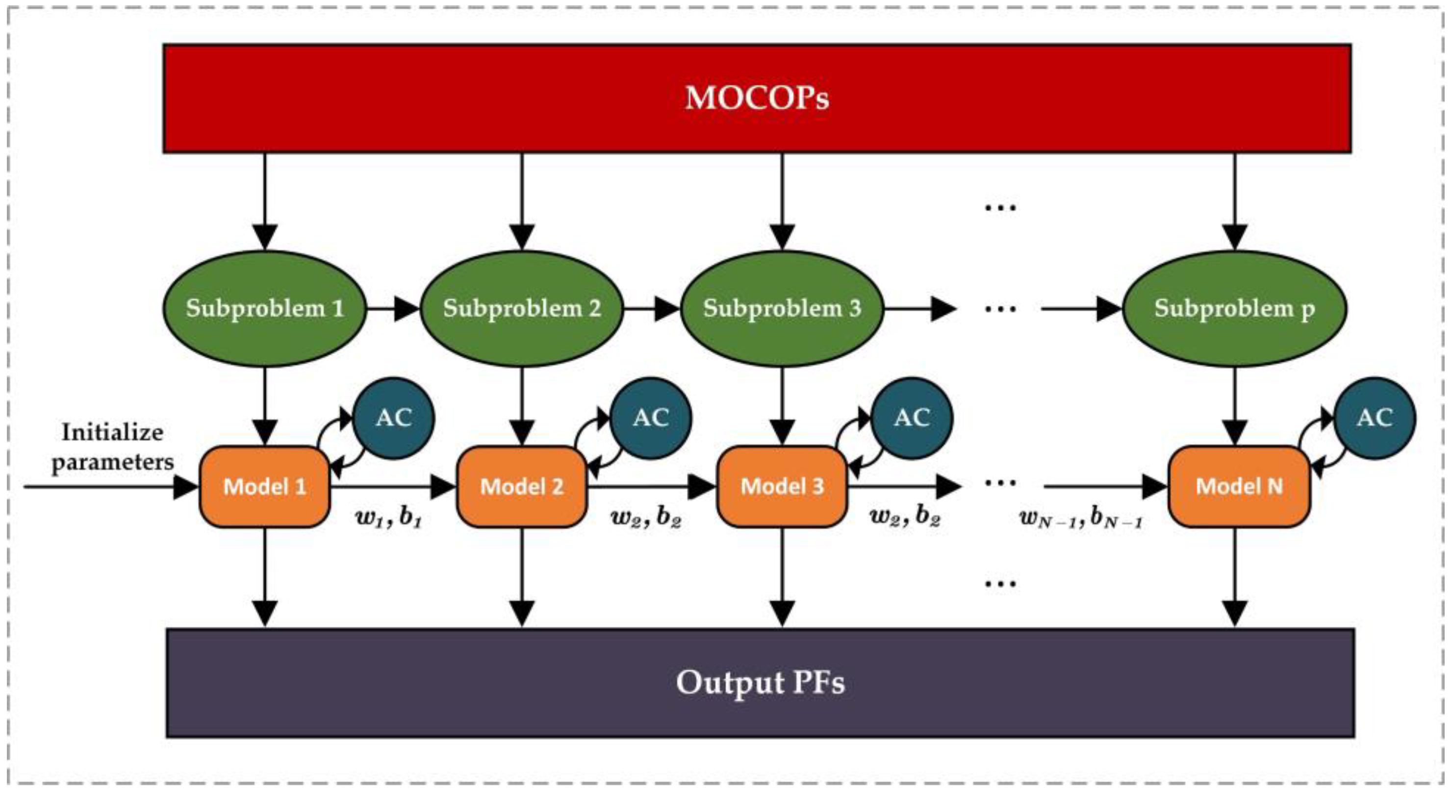
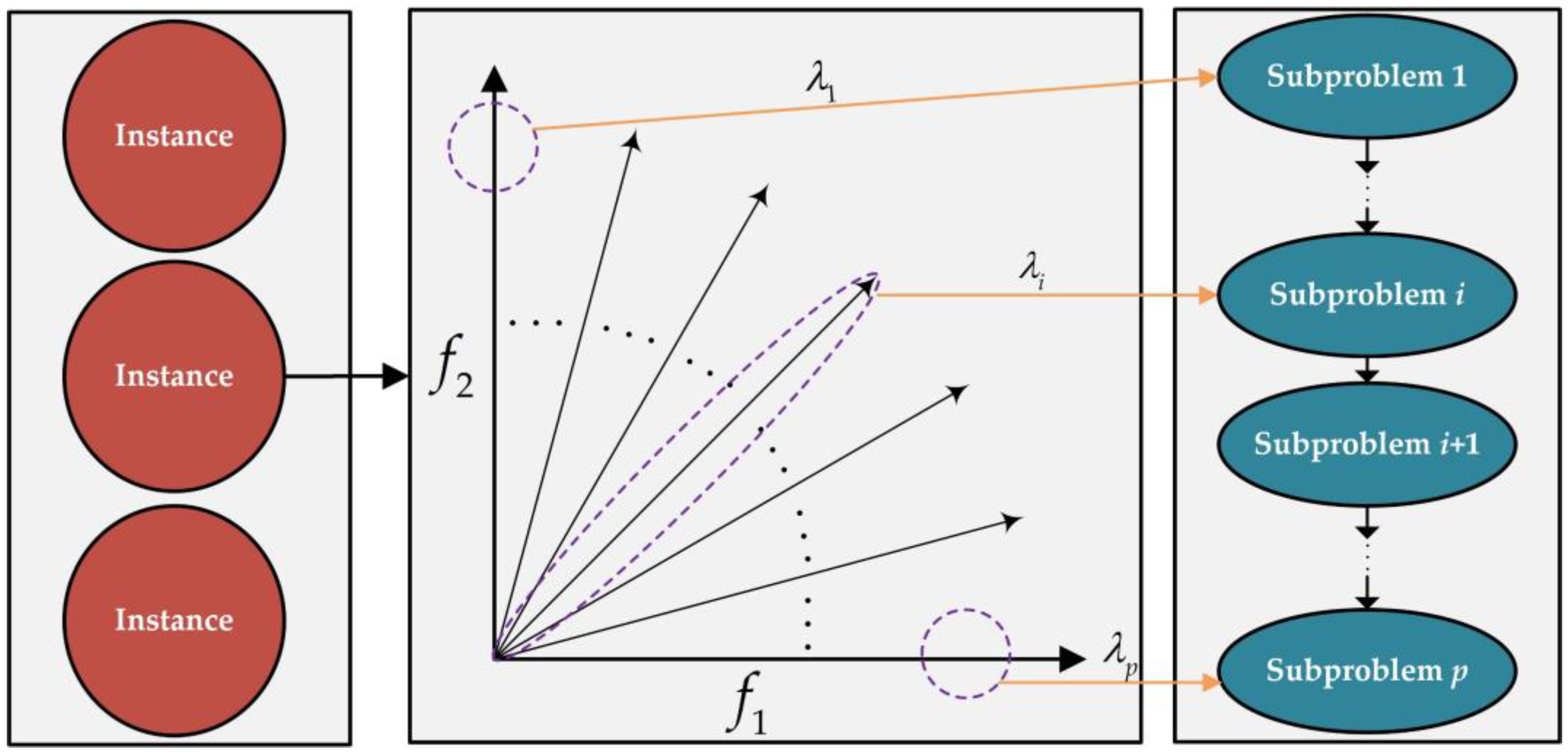
2.3. Overview of DRL-MOA

The process of the DRL-MOA algorithm is shown in Figure 1. It is set against the backdrop of the Euclidean bi-objective traveling salesman problem for the DRL algorithm, involving $m$ optimization objectives and n city nodes. A set of city nodes is defined as $X_{node}=\left\{x_1,x_2,\dots ,x_n\right\}$, where $x_n$ represents all information about the n-th city node, which is constituted by the feature vector $\left(x_n^1,x_n^2,\dots ,x_n^m\right)$, with $x_n^m=(s_n^m,s_n^{*m})$. The visiting order of the cities by the salesman, $S=\left(s_1,s_{2,}\dots ,s_n\right)$, serves as the solution.

DRL-MOA draws inspiration from the weight and decomposition methods of MOEA/D. As shown in Figure 2, the MOTSP problem with $m$ optimization objectives is decomposed into $p$ sub-problems, and a set of weight vectors ${\lambda }_{1,}{\lambda }_{2,}\dots {\lambda }_p$ is associated with each sub-problem, where ${\lambda }_i={\left({\lambda }_i^1,{\lambda }_i^2,\dots ,{\lambda }_i^m\right)}^{\mathsf{{\rm T}}}$, and satisfies $i\in \left\{\mathrm{1,2},\dots ,p\right\}$. The objective function formula for the $j$-th sub-problem can be described as follows:

$$g^{ws}\left(x|{\lambda }_i^j\right)=\sum _{j=1}^m{\lambda }_i^j{f}_j\left(x\right).$$

(3)

From the above analysis, DRL-MOA has transformed the optimization of a multi-objective problem into the optimization of $p$ sub-problems. Since adjacent weight vectors corresponding to sub-problems have certain similarities, by transferring the model parameters directly from one sub-problem to the next after completing the current one, the efficiency of model training can be greatly improved.

As illustrated in Figure 3, the DRL-MOA algorithm uses the actor–critic network [57] architecture for the training of its sub-models. Within this framework, the actor is responsible for making decisions under specific environmental states, that is, selecting the next target city while taking into account the current and unvisited cities. The critic, meanwhile, is tasked with evaluating each of the actor’s decisions, providing continuous guidance on strategy adjustment by estimating the potential returns of specific actions under the current state. Moreover, the critic gradually optimizes its evaluation strategy through constant interaction with the environment, thereby more effectively guiding the actor in adjusting its action plan.

The actor–critic network employs an end-to-end training approach using the pointer network model, as shown in Figure 4. The core idea is to use the encoder to encode the input sequence into feature vectors and then use the decoder combined with the attention calculation method to construct the solution step by step in an autoregressive manner—that is, each time a node is selected based on the nodes already chosen until a complete solution is constructed. The encoder uses one-dimensional convolution to transform the node features and map them to a high-dimensional vector space, eventually storing all the input sequence information in vector $C$. During the decoding phase, a probability distribution is generated by the GRU and attention mechanism, and the solution is gradually formed. At each decoding step $t=\left\{\mathrm{1,2},\dots ,n\right\}$, an unvisited city node is selected. The attention mechanism is responsible for calculating the relevance of each input at the next decoding step $t$, with the most relevant city being the most likely to be selected. The formula for selecting the next city can be described as follows:

$$q_j^t={\alpha }^{\mathrm{T}}tanh\left(W_1{e}_j+W_2{d}_t\right),j=\mathrm{1,2},\dots ,n .$$

(4)

where $q_j^t$ represents the relevance of the $j$-th city node at the $t$-th selection, and $\partial$, $W_1$, and $W_2$ represent learnable parameters of the network, $e_j$ denotes the hidden state of the $j$-th city node, $d_t$ denotes the hidden state of the decoder at step $t$, and $X_t$ represents the set of city nodes that have not been visited. During training, the model selects the next city by sampling from the probability distribution. The process of generating output $S$ from input $X_{node}$ can be described by the following formula:

$$P\left(S|X_{node}\right)=\prod _{t=1}^{n}P\left(s_{t+1}|s_{1,}\dots ,s_t,X_t\right).$$

(5)

In DRL-MOA, the encoder extracts node features using a simple one-dimensional convolutional layer and fails to effectively capture the graph structure of problem instances defined on fully connected graphs. During the decoding stage, a probability distribution is generated based on partial paths to select the next node, but this method does not adequately consider the specific constraints of path selection in MOTSP, where choosing the next node is only related to the first and last nodes of the partial path, resulting in generated hidden states containing a large amount of unnecessary information.

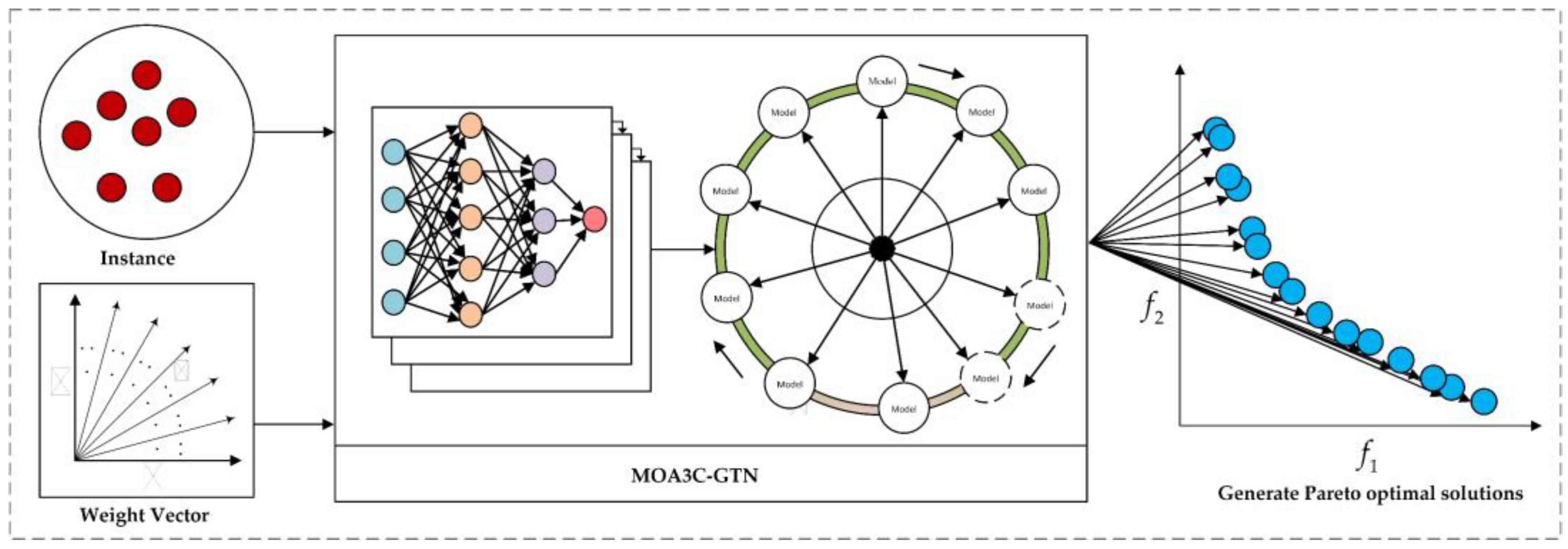
3. MOA3C-GTN Algorithm

In this section, we introduce the solution process of MOA3C-GTN, the enhanced GTN architecture, and the A3C training mode.

3.1. General Solution Process

Figure 5 illustrates the solving process of the MOA3C-GTN algorithm as described. The solving process of MOA3C-GTN proposed in this section decomposes the MOCOP problem into $Q$ individual COPs using the method of uniform weight decomposition. Algorithm 1 provides a detailed outline of this process. For each weight vector’s sub-problem, denoted by ${\lambda }_i$ where $i\in \left\{\mathrm{1,2},\dots ,Q\right\}$, the model takes as input the node information $X_{node}$ and the weight vector ${\lambda }_i$. It then computes a solution and adds it to the set $P_1^{*}$. After completing this process $Q$ times, the Pareto optimal solution set $P^{*}$ is calculated [58,59,60].

Algorithm 1 General framework of MOA3C-GTN

Input: Node information $X_{node}$, weight vectors ${\lambda }_1,{\lambda }_2,\dots ,{\lambda }_Q$.

Output: Pareto optimal solution set $P^{\mathrm{*}}.$

1 Pareto optimal solution set: $P^{\mathrm{*}}\leftarrow \mathrm{\varnothing }$$, P_1^{\mathrm{*}}\leftarrow \mathrm{\varnothing }$

2 for $i=1:Q$ do

3  $S\leftarrow \mathrm{M}\mathrm{O}\mathrm{A}3\mathrm{C}-\mathrm{G}\mathrm{T}\mathrm{N}\mathrm{s}\left(X_{node},{\lambda }_i\right)$

4  $P_1^{\mathrm{*}}\leftarrow P_1^{\mathrm{*}}\cup \left\{S\right\}$

5 end for

6 Select Pareto optimal solution set: $P^{\mathrm{*}}\leftarrow P_1^{\mathrm{*}}$

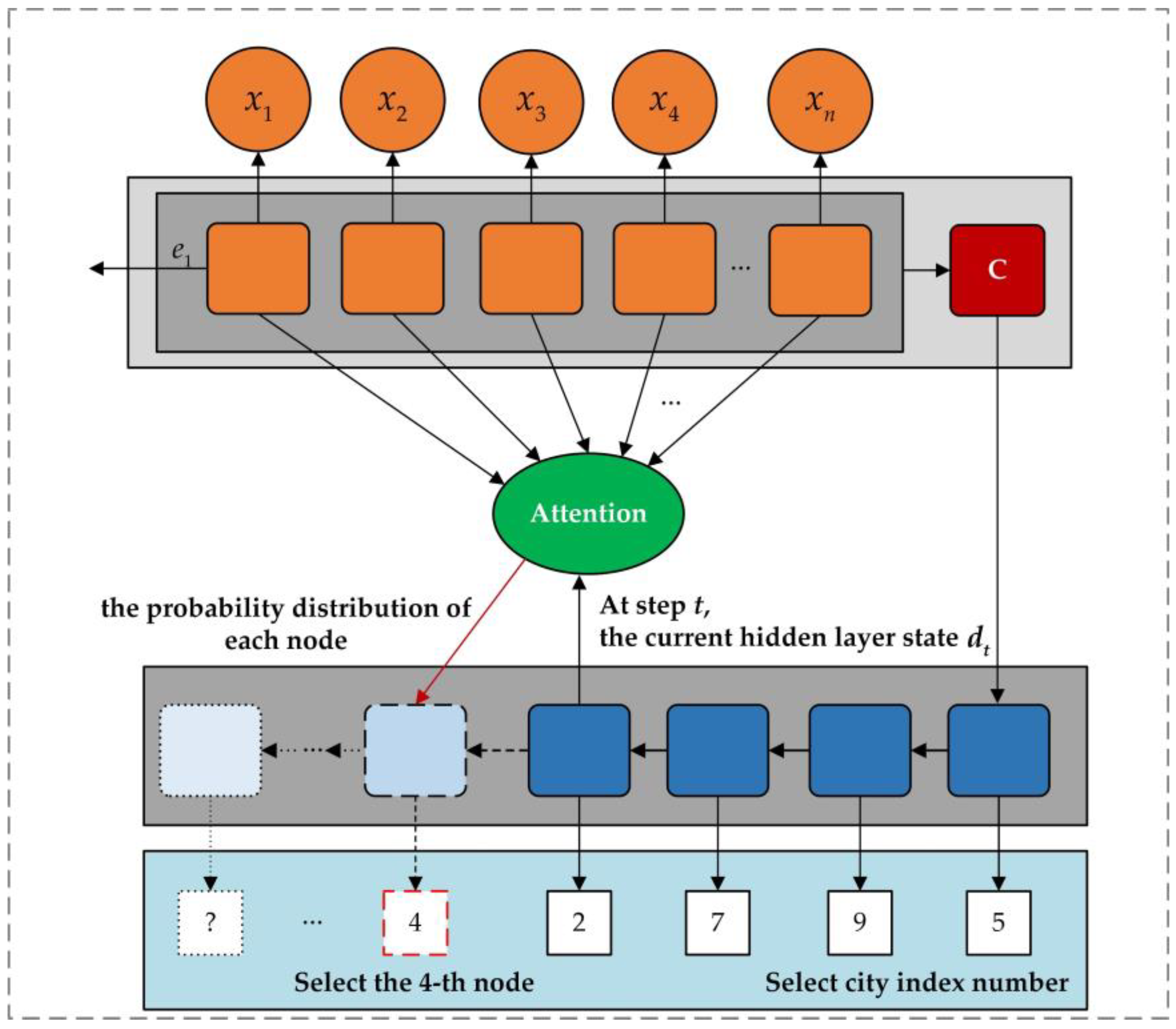
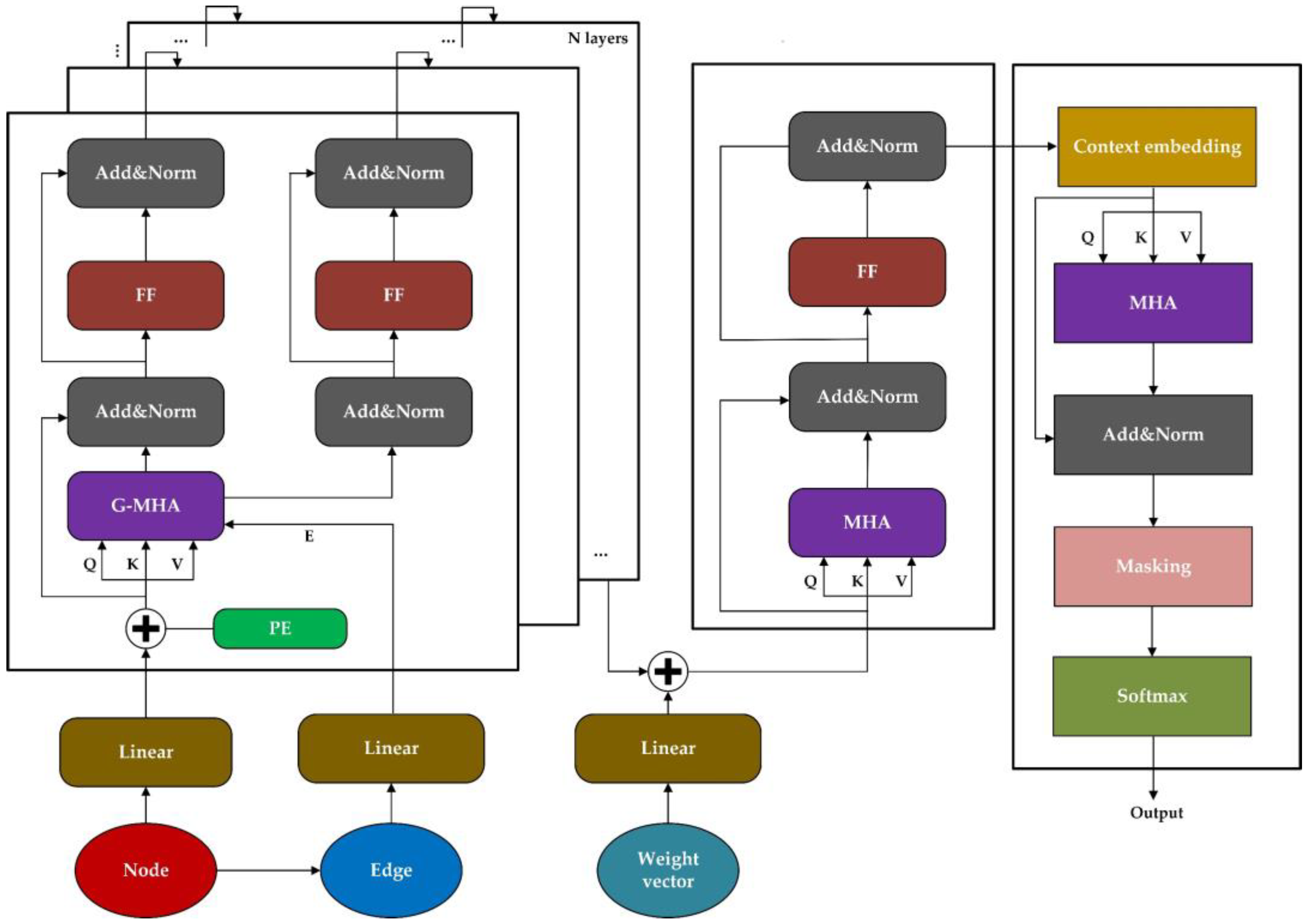
3.2. Graph Transformer Network Integrating Node, Edge, and Target Weight Information

In this section, we propose a GTN architecture that simultaneously considers the vertex information, edge information, and target weight information, as shown in Figure 6.

The encoder consists of a node-encoding layer and a weight-encoding layer. The node-encoding layer generates embeddings for node information $\left\{x_1,x_2,\dots ,x_n\right\}$ and calculates the edge information from the city information of the nodes, embedding the edge information accordingly. The weight-encoding layer embeds the weight vector information $\left\{{\lambda }_1,{\lambda }_2,\dots ,{\lambda }_P\right\}$.

The node information is mapped through a linear embedding layer and added to positional encoding embeddings, while the edge information is directly embedded through a linear embedding layer. The specific operations for the embeddings can be described as follows, where $l\in \left\{\mathrm{1,2},3,\dots ,N\right\}$ denotes the $l$-th encoding layer, $i$ indicates the position of node encoding, and d_model represents the dimension of embedding:

$$h_i^{l^{\prime }}=A^l{x}_i^l+a^l,$$

(6)

$$P{E}_{i,l}=\left\{\begin{array}{c}\mathit{sin}(i\cdot 10000^{{\displaystyle \frac{d_{model}}{2l}}}),i=2k\\ \mathit{cos}(i\cdot 10000^{{\displaystyle \frac{d_{model}}{2l}}}),i=2k+1\end{array}\right.,$$

(7)

$$h_i^l=h_i^{l^{\prime }}+P{E}_{i,l},$$

(8)

$$e_{ij}^l=B^l{\tilde{e}}_{ij}^l+b^l.$$

(9)

The processed vectors are embedded into the multi-head attention (MHA) layer. where the outputs of the attention mechanism, denoted as ${\mathrm{A}}^h$, are concatenated and subsequently projected onto the space $W_0\in R^{d_{model}\times d_{model}}$. The operations within the MHA layer are described as follows:

$$\mathrm{NMHA}\left(Q,K,V,E\right)=\mathrm{Concat}\left({\mathrm{A}}^1{\mathrm{E}}^1,{\mathrm{A}}^2{\mathrm{E}}^2,\dots ,{\mathrm{A}}^H{\mathrm{E}}^H\right)W_N,$$

(10)

$${\mathrm{A}}^h=\mathrm{ATTEN}\left(W_Q^h{Q}^h,W_K^h{K}^h,W_V^h{V}^h,W_E^h{E}^h\right),$$

(11)

$$\mathrm{ATTEN}\left(Q^h,K^h,V^h,E^h\right)=\mathrm{softmax}\left({\displaystyle \frac{Q^h{K}^{h^{\mathsf{{\rm T}}}}{E}^h}{\sqrt{d_h}}}\right)\cdot V^h,$$

(12)

$$\mathrm{EMHA}\left(Q,K,E\right)=\mathrm{Concat}\left({\displaystyle \frac{Q^1{K}^{1^{\mathsf{{\rm T}}}}{E}^1}{\sqrt{d_1}}},{\displaystyle \frac{Q^2{K}^{2^{\mathsf{{\rm T}}}}{E}^2}{\sqrt{d_2}}},\dots ,{\displaystyle \frac{Q^H{K}^{H^{\mathsf{{\rm T}}}}{E}^H}{\sqrt{d_H}}}\right)W_E.$$

(13)

where NMHA and EMHA represent the multi-head attention mechanisms for the nodes and edges, respectively. $Q$, $K$, and $V$ denote the query, key, and value vectors, while $E^h\in {\mathbb{R}}^{d_h\times d_{\mathrm{model}}}$, where $h\in \left\{\mathrm{1,2},3,\dots ,H\right\}$, indexes the number of heads in the attention mechanism. Each head computes attention based on the transformed queries, keys, values, and edge vectors, and the softmax function is applied to the scaled dot products of the queries and keys. This structure enhances the model’s ability to focus on relevant features by dynamically adjusting the attention based on both node attributes and the relationships (edges) between them.

The MHA layer outputs are forwarded to a batch normalization (BN) network layer, activated by the nonlinear ReLU function, before passing through a feed forward (FF) network layer. Subsequently, the BN layer processes the output encoding vectors again. The detailed operations can be described as follows:

$$\widehat{h_i^l}=\mathrm{B}\mathrm{N}\left(h_i^{l-1}+\mathrm{NMH}{\mathrm{A}}_i^l\left(Q,K,V,E\right)\right),$$

(14)

$$h_i^l=\mathrm{B}\mathrm{N}\left(\widehat{h_i^l}+\mathrm{F}\mathrm{F}\left(\widehat{h_i^l}\right)\right),$$

(15)

$$\widehat{e_{ij}^l}=\mathrm{B}\mathrm{N}\left(e_{ij}^{l-1}+\mathrm{E}\mathrm{M}\mathrm{H}{\mathrm{A}}_{\mathrm{i}\mathrm{j}}^{\mathrm{l}}\left(Q,K,E\right)\right)$$

(16)

$$e_{ij}^l=\mathrm{B}\mathrm{N}\left(\widehat{e_{ij}^l}+\mathrm{F}\mathrm{F}\left(\widehat{e_{ij}^l}\right)\right).$$

(17)

Located beneath the node-encoding layer, the weight-encoding layer embeds the weight vectors as follows:

$${\rm E}=W_{\lambda }\lambda +b_{\lambda },$$

(18)

$$h_t^{\lambda }=E{h}_t^N+b_t^N.$$

(19)

where $E$ represents the embedding of weight vectors, while $W_{\lambda }$ and $b_{\lambda }$ are learnable parameters. These operations facilitate the encoding of the city node and weight information into sequential vectors, which are then processed by the decoder for graph embedding, point embedding, contextual vector generation, and masking. This process outputs the probabilities for selecting the next node until a complete solution $S$ is formed when all nodes have been selected. This sophisticated processing sequence ensures the dynamic and efficient handling of the node and edge information within the neural network architecture, crucial for tasks involving sequential decision making and pattern recognition within graph-structured data.

After encoding the city node and weight information into sequential vectors, the encoder passes these into the decoder to handle graph embedding, point embedding, contextual vector, and masking, subsequently outputting the probability of selecting the next node until all nodes are chosen, forming a solution $S$.

The introduction of a contextual node $c$ allows for the initial node selection through multiple random starting points, enhanced by a masking technique to prevent re-visiting nodes, thereby effectively calculating the attention allocation for the encoded nodes and probabilistically outputting the next city node to visit. The context embedding comprises three parts: the graph embedding from the encoding layer $\overline{h^{N+1}}$, the initial node $h_{s_1}^{N+1}$, and the prior node $h_{s_{t-1}}^{N+1}$. The context embedding at time $t$ can be described as follows:

$$h_c^{N+1}=\left\{\begin{array}{cc}\left[\overline{h^{N+1}},h_{s_{t-1}}^{N+1},h_{s_1}^{N+1}\right],& t>1\\ none,& t=1\end{array}\right..$$

(20)

When $t=1$, the decoder does not control the selection of the first node; instead, $N$ distinct context node embeddings are used. The feature vectors are computed using a multi-head attention mechanism with node embeddings to obtain a new context embedding $l_c$. The query vector $q_c$ and the key vector $k_i$ originate from the context embedding $l_c$ and $h_c^{N+1}$, respectively. The expressions for the context embedding $l_c$, query vector $q_c$, and key vector $k_i$ are as follows:

$$l_c=\mathrm{M}\mathrm{H}\mathrm{A}\left(\left\{h_1^{N+1},h_2^{N+1},\dots ,h_n^{N+1}\right\},h_c^{N+1}\right),$$

(21)

$$q_c=W_Q{l}_c,$$

(22)

$$k_i=W_K{h}_c.$$

(23)

Incorporating masking technology effectively computes the attention allocation for encoded nodes, maximizing the probability of outputting the next city node to be visited:

$$u_{cj}=\left\{\begin{array}{cc}C·\mathit{tanh}\left(q_c^T{k}_j\right),& if j\ne s_{t^{\prime }},\forall t^{\prime }<t\\ -\mathrm{\infty },& otherwise.\end{array}\right.,$$

(24)

$$p_i=p_{\theta }\left(s_t|s_{1:t-1},\lambda ,X_{node}\right)=\mathrm{softmax}\left({\displaystyle \frac{e^{u_{ci}}}{\sum j{e}^{uj}}}\right).$$

(25)

where $u_{cj}$ denotes the importance of each node’s new context embedding, and $p_i$ represents the probability distribution for selecting the next city. Thus, by utilizing the softmax function, the probabilities of selecting each node are computed and outputted. This method ensures dynamic attention allocation based on contextual embeddings, enhancing the efficiency and accuracy of the node selection in sequential decision-making tasks within graph-based models.

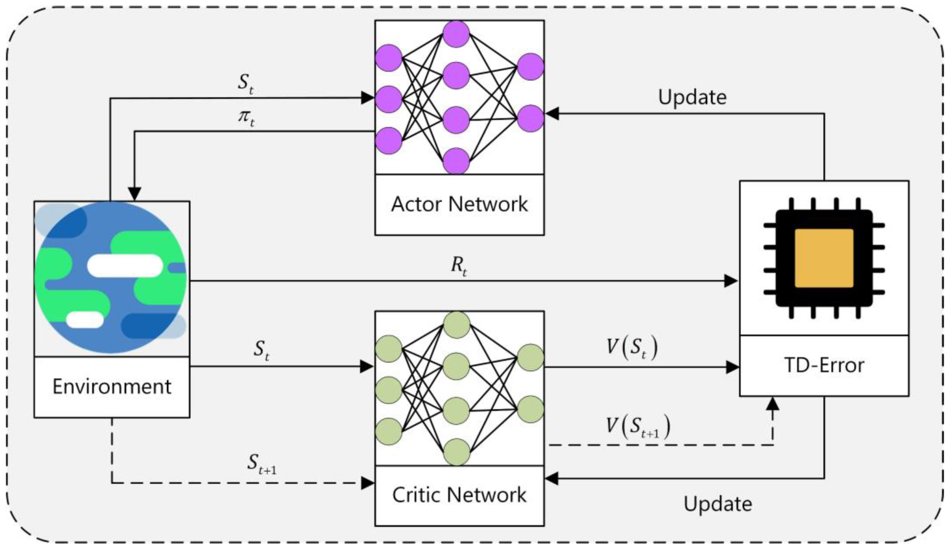
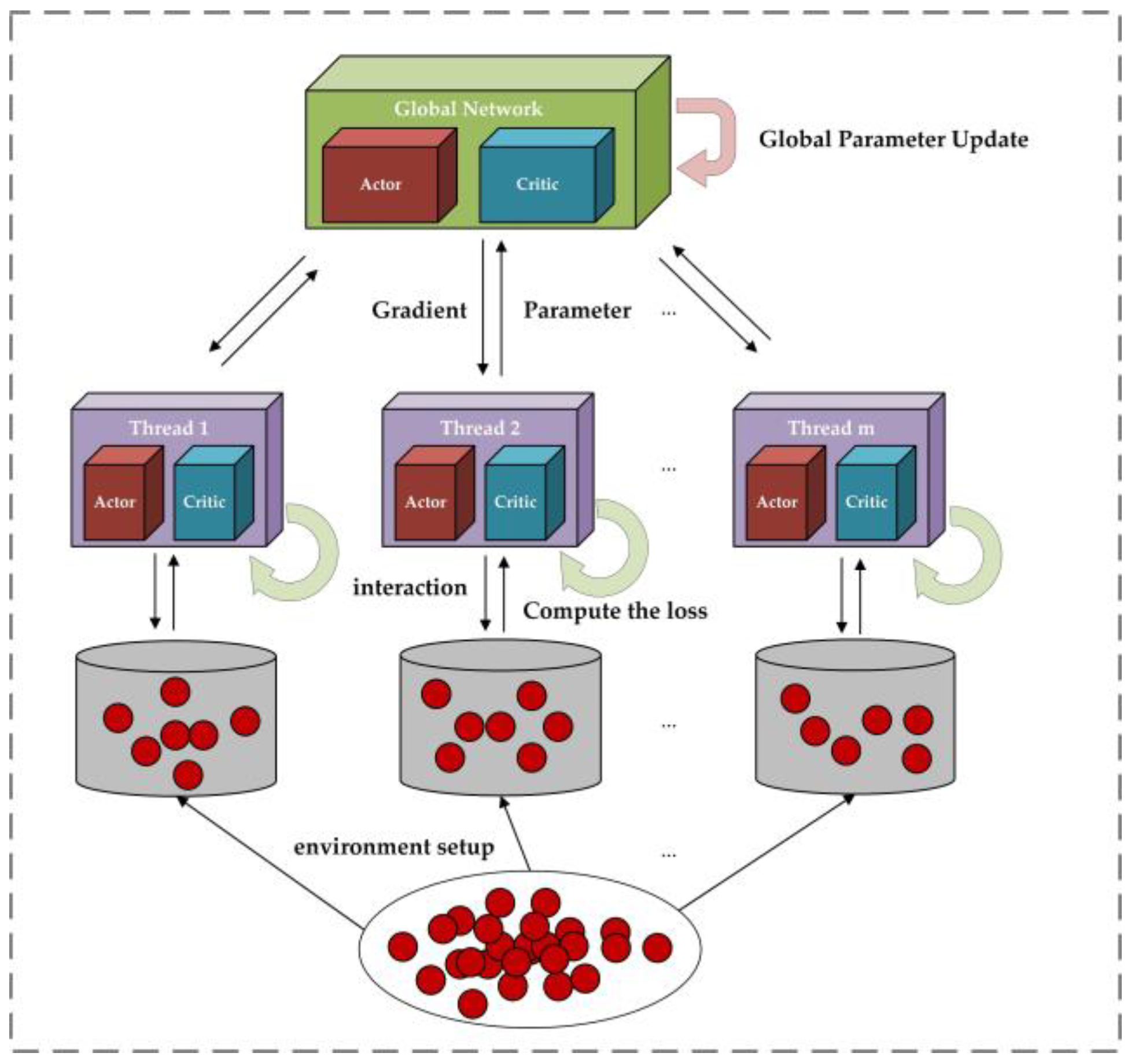
3.3. A3C Training Mode

The sub-problem model is trained using the A3C method [61,62,63]. By setting up multiple workers operating in a multi-threaded environment to select paths, we can avoid the pitfalls of backtracking from large-scale and randomly generated data and steer clear of local optima, as shown in Figure 7. Each worker performs policy execution and gradient computation locally and then updates the global actor and critic asynchronously.

Algorithm 2 describes the training steps of a thread within the A3C network. The algorithm begins by initializing the global network parameters $\theta$ and $\varphi$, then enters a nested loop structure—where the outer loop iterates over each training epoch and the inner loop over each step within the epoch. In each step, the algorithm resets the gradients $d\theta$ and $d\varphi$, and synchronizes the global network parameters $\theta$ and $\varphi$ to each thread. Then, for each batch $b$, it samples $D_b$ from the dataset $D$ and ${\lambda }_b$ from the weight vector λ, acts according to the actor network’s parameters ${\theta }^{\prime }$ within the current thread to choose routes ${\pi }_b$, evaluates the value of the action $c_b$ according to the critic network’s parameters ${\theta }^{\prime }$, and computes the reward $R_b$. After this, it updates the local gradients for both the actor and critic networks. Finally, the global network parameters $\theta$ and $\varphi$ are updated asynchronously using the ADAM optimizer. Through the repeated iteration of these steps, the global network parameters are gradually optimized, thereby improving the training efficiency and effectiveness of the model in a multi-threaded environment.

Algorithm 2 Asynchronous advantage actor–critic network training algorithm

Input: Number of training epochs $E$, number of steps per training epoch $T$, batch size $B$, significance level $\partial$, dataset $D$, weight vector $\lambda$, global network parameters for actor $\theta$, global network parameters for critic $\varphi$, local network parameters for actor ${\theta }^{\prime }$, local network parameters for critic ${\varphi }^{\prime }$.

Output: Global network parameters for actor $\theta$, global network parameters for critic $\varphi$.

1 Initialize global network parameters: $\theta$$,\varphi$

2 for $e=1:E$ do

3   for $t=1:T$ do

4     Reset gradients: $d\theta \leftarrow 0,d\varphi \leftarrow 0$

5     Synchronize parameters: ${\theta }^{\prime }=\theta ,{\varphi }^{\prime }=\varphi$

6     $D_b\leftarrow \mathrm{S}\mathrm{a}\mathrm{m}\mathrm{p}\mathrm{l}\mathrm{e}\mathrm{I}\mathrm{n}\mathrm{p}\mathrm{u}\mathrm{t}\left(D\right)$$,{\lambda }_b\leftarrow \mathrm{S}\mathrm{a}\mathrm{m}\mathrm{p}\mathrm{l}\mathrm{e}\mathrm{I}\mathrm{n}\mathrm{p}\mathrm{u}\mathrm{t}\left(\lambda \right)$$,\forall b\in \left\{\mathrm{1,2},\dots ,B\right\}$

7     ${\pi }_b\leftarrow SampleRollout\left(D_b,{\lambda }_b,P_{{\theta }^{\prime }}\right)$$,\forall b\in \left\{\mathrm{1,2},\dots ,B\right\}$

8     $c_b\leftarrow c_{\varphi }\left(D_b,{\lambda }_b\right)$$, \forall b\in \left\{\mathrm{1,2},\dots ,B\right\}$

9     Compute reward $R_b$$,\forall b\in \left\{\mathrm{1,2},\dots ,B\right\}$

10     Update gradient: $d\theta \leftarrow {\displaystyle \frac{1}{B}}{\sum }_{b=1}^B\left[\left(R_b-c_b\right){\nabla }_{{\theta }^{\prime }}\mathit{log}{P}_{{\theta }^{\prime }}\left({\pi }_b\right)\right]$

11     Update gradient: $d\varphi \leftarrow {\displaystyle \frac{\partial }{B}}{{\sum }_{b=1}^B\left(R_b-c_b\right)}^2$

12     Asynchronous update operation: $\theta \leftarrow ADAM\left(\theta ,d\theta \right)$, $\varphi \leftarrow ADAM\left(\varphi ,d\varphi \right)$

13   end for

14 end for

3.4. Complexity Analysis

The time complexity of the MOA3C-GTN algorithm is influenced by two main factors: the A3C method and the GTN architecture.

The time complexity of the A3C component largely depends on the number of parallel working threads. In the A3C model, each thread operates independently and processes a fixed number of time steps. Assuming there are $N$ parallel threads, each handling $T$ time steps, the time complexity of A3C would be approximately $O(T\cdot N)$. This parallel computation approach significantly enhances the efficiency of model training. The GTN architecture, which incorporates the node information, edge information, and target weight information, performs a deep encoding of the graph structure data. The time complexity associated with the GTN depends on the number of nodes $V$, the number of edges $E$, and the depth of the network layers $D$, generally scaling as $O\left(\right(V+E)\cdot D)$.

Regarding space complexity, A3C requires storage for the policy and value network parameters of each thread, leading to a space complexity of about $O(N\cdot S)$, where S represents the total number of network parameters. The GTN architecture necessitates additional storage for the features of each node and edge, as well as the associated weights. Assuming a feature dimension $F$ for each node and edge, the space complexity for GTNs is $O\left(\right(V+E)\cdot F)$. Thus, the overall space complexity of the algorithm is $O\left(\right(V+E)\cdot F+N\cdot S)$. This indicates that handling large-scale graph structures with many nodes and edges may require substantial storage space. These complexity analyses help us better understand the algorithm’s performance and resource demands in practical applications.

4. Results

This section is divided into two subsections: the experimental setup and the results analysis.

4.1. Experimental Setup

The testing problem adopted in this experiment is the Euclidean instance of the bi-objective traveling salesman problem, where both optimization objectives are path lengths. The traveling cost is defined as the Euclidean distance between any two nodes. The first optimization objective considers the traveling cost between the actual coordinates of the nodes, while the second optimization objective is based on the cost between the virtual coordinates of the nodes.

The MOA3C-GTN algorithm is compared with several existing algorithms, including the DRL-MOA, MODRL/D-AM, ML-AM, and MODRL/D-EL algorithms based on DRL, as well as traditional multi-objective evolutionary algorithms such as MOEA/D (2000 iterations) and NSGA-II (2000 iterations). MODMAM, which utilizes multiple decoders to generate and select multiple solutions for each weight problem, runs approximately 2.7 times faster than the DRL-MOA algorithm. However, the present algorithm is based on a non-multiple decoder mechanism; thus, it is not compared with the MODMAM algorithm on Pareto fronts.

The experiments are conducted on a computer equipped with an Intel Core i7-13700K processor and an NVIDIA GeForce RTX 4070 graphics card. All algorithms are executed on the PlatEMO platform (version 4.1) [64].

During training, the batch size is set to 200, the size of problem instances is set to 500,000, and the problem scale of the model training set is fixed to 30 cities (previous experimental training problem scales were 40 cities), with 100 sub-problems (100 weight vectors). Nodes are embedded into 128-dimensional vectors. The encoder consists of six layers of node encoding, each layer with a feature dimension of 128. Each encoding layer is equipped with six attention heads, and the hidden layer dimension of the fully connected layer is set to 512. In the weight-encoding layer, weight vectors are first transformed into 128-dimensional vectors, then processed together with node embeddings, with hyperparameters set the same as those of the node-encoding layer. Each decoder accepts a 128-dimensional vector input and adopts a six-head attention mechanism.

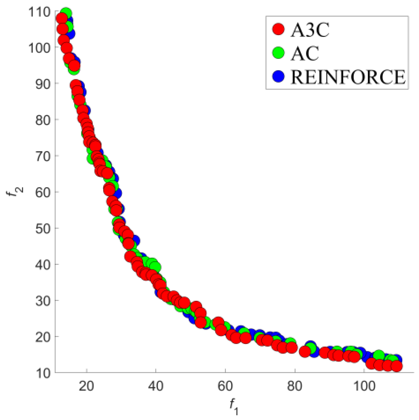
4.2. Results and Discussion

In this study, we assessed the performance and efficiency of the MOA3C-GTN algorithm by comparing it with six other multi-objective optimization algorithms—including MOEA/D, NSGA-II, DRL-MOA, MODRL/D-AM, ML-AM, and MODRL/D-EL—across different scales of bi-objective traveling salesman problems. Tests were conducted on random instances involving 40, 70, 100, 150, and 200 cities, as depicted in Figure 8,

Table 2. Hypervolume comparison.

	MOA3C-GTN	MOEA/D	NSGA-II	DRL-MOA	MODRL/D-AM	ML-AM	MODRL/D-EL
40-city	0.6875	0.6375	0.6256	0.6493	0.6512	0.6751	0.6812
70-city	0.7292	0.6651	0.6330	0.6926	0.6921	0.7074	0.7147
100-city	0.7586	0.6327	0.6159	0.7027	0.751	0.7212	0.7337
150-city	0.7845	0.6216	0.6122	0.7397	0.7524	0.7565	0.7612
200-city	0.8334	0.6543	0.6318	0.7670	0.7817	0.7112	0.8278

and

Table 3. Runtime comparison.

	MOA3C-GTN	MOEA/D	NSGA-II	DRL-MOA	MODRL/D-AM	ML-AM	MODRL/D-EL
40-city	3.45	67.99	13.47	2.52	5.06	3.528	6.47
70-city	6.62	70.32	16.02	4.71	8.25	6.58	10.87
100-city	12.01	73.98	28.75	7.24	13.08	11.58	17.62
150-city	15.87	78.82	21.41	9.72	19.44	14.60	24.13
200-city	28.07	82.42	23.04	13.18	26.39	18.44	30.19

.

The results demonstrate that the MOA3C-GTN algorithm exhibited superior performance across all problem instances. Notably, in large-scale instances (150 and 200 cities), MOA3C-GTN found solutions that were closer to the true Pareto front compared to other algorithms. This achievement highlights the potential of MOA3C-GTN in managing complex multi-objective problems, particularly when a significant number of decision variables are involved. As the problem size increased, MOA3C-GTN displayed remarkable robustness, while other algorithms experienced more pronounced impacts on the solution quality and convergence speed. Traditional algorithms, despite performing comparably with deep-learning-based algorithms for medium-scale problems (70 and 100 cities), showed declining performance at larger scales.

Regarding the algorithm runtime, MOA3C-GTN also demonstrated efficiency. For example, it only took 3.45 s to run on a 40-city problem, substantially less than MOEA/D’s 67.99 s and NSGA-II’s 13.47 s. As the city size increased to 200, MOA3C-GTN’s runtime was merely 28.07 s, notably less than MOEA/D’s 82.42 s and MODRL/D-EL’s 30.19 s, showcasing its significant time efficiency advantage.

MOA3C-GTN consistently achieved the highest hypervolume (HV) metric [65] across all tested city sizes, underscoring its exceptional performance in multi-objective optimization. For instance, in the 200-city scenario, MOA3C-GTN’s HV value reached 0.8334, significantly surpassing other algorithms.

Additionally, we conducted two ablation experiments to verify the design details of the algorithm. The first experiment explored the effect of considering edge information in GTN, and the second compared the performance of the A3C, REINFORCE, and actor–critic training modes.

The experimental results indicated that the GTN incorporating edge information improved both the quantity and quality of solutions, confirming its effectiveness. Solutions using the A3C training mode were slightly superior in quality compared to the other methods, suggesting that A3C can effectively avoid local optima and better locate optimal solutions for each weight vector.

Moreover, we set up two ablation studies: the first to verify the effectiveness of considering edge information in GTNs for solving PFs, and the second to confirm the superiority of the A3C training mode in solution set quality over the REINFORCE and actor-centric methods.

Introducing edge information in the GTN significantly enhanced algorithm performance. As illustrated in Figure 9, the red points (with edge information) were superior to the blue points (without edge information) in the majority of cases, particularly in regions with lower objective values, indicating better optimization results. This demonstrates that incorporating edge information can effectively enhance the algorithm’s exploratory capabilities and solution quality, especially in dealing with complex or information-rich multi-objective combinatorial optimization problems, guiding the search process more accurately towards solutions closer to the Pareto front.

In experiments comparing the A3C, REINFORCE, and actor-centric training modes, as shown in Figure 10, A3C (red points) covered a wider area with a more uniform distribution, displaying superior performance over the other methods (green and blue points). Particularly in regions with lower objective values, A3C utilized its asynchronous training advantage to more frequently find superior solutions, indicating that A3C’s asynchronous advantage and comprehensive update strategy significantly enhance the algorithm’s global search capability and convergence speed. This training mode helps the algorithm avoid local optima and effectively enhances solution stability and reliability in complex search spaces.

Overall, these results not only confirm the advanced design of MOA3C-GTN but also validate its potential for practical application, especially in scenarios that require the consideration of both solution quality and operational efficiency. MOA3C-GTN can generate high-quality solution sets in a short time, significantly standing out in the field of multi-objective optimization and offering substantial practical value for addressing real-world complex problems.

5. Conclusions

In recent years, DRL methods proposed in the field of MOPs have some drawbacks, such as slow speed, slow convergence, and the inability to flexibly adapt to new objective weight vectors. A multi-objective combinatorial optimization algorithm, named MOA3C-GTN, is proposed herein, aiming to overcome the limitations of traditional algorithms in addressing complex multi-objective problems by integrating DRL and graph transformation network techniques. The utilization of the A3C in this algorithm, as opposed to the traditional REINFORCE method, effectively reduces the variance in the learning process and prevents the algorithm from being trapped in local optima. Furthermore, the introduction of an architecture based on graph transformation networks within MOA3C-GTN, capable of extending to edge feature representation, accurately captures the topological properties of graph structures and the latent relationships between nodes, thereby significantly enhancing the algorithm’s expressiveness and flexibility.

In empirical studies, this algorithm demonstrates outstanding performance in addressing the bi-objective traveling salesman problem, exhibiting clear advantages over the recent research in the same field, particularly in terms of training efficiency and solution diversity. However, the applicability of this algorithm to a broader range of multi-objective combinatorial optimization problems requires further validation. Considering future research directions, exploring the effectiveness of this algorithm in different complex scenarios and contemplating the introduction of novel network structures and optimization strategies to enhance algorithm performance remains a pertinent issue. Additionally, the prospect of integrating other machine-learning techniques represents a crucial avenue for future research, with the anticipation of discovering more innovative solutions to tackle the challenges posed by multi-objective optimization problems.

References

1. Ahmed, F.; Deb, K. Multi-objective optimal path planning using elitist non-dominated sorting genetic algorithms. Soft Comput. 2013, 17, 1283–1299. [Google Scholar] [CrossRef]
2. Sun, J.; Gan, X.J.; Gong, D.W.; Tang, X.K.; Dai, H.W.; Zhong, Z.M. A self-evolving fuzzy system online prediction-based dynamic multi-objective evolutionary algorithm. Inf. Sci. 2022, 612, 638–654. [Google Scholar] [CrossRef]
3. Zhu, Y.; Chen, Y.; Huray, P.; Dong, X. Evolutionary Algorithms for Multiobjective Optimization. Sci. Technol. Inf. 2008, 4, 59–68. [Google Scholar] [CrossRef]
4. Gan, X.J.; Sun, J.; Gong, D.W.; Jia, D.B.; Dai, H.W.; Zhong, Z.M. An adaptive reference vector based interval multi-objective evolutionary algorithm. IEEE Trans. Evol. Comput. 2023, 27, 1235–1249. [Google Scholar] [CrossRef]
5. Oumayma, B.; Talbi, E.G.; Nahla, B.A. Using Possibility Theory to Solve a Multi-Objective Combinatorial Problem under Uncertainty: Definition of New Pareto-Optimality. Available online: https://scholar.google.fr/citations?view_op=view_citation&hl=fr&user=TM0z7KQAAAAJ&citation_for_view=TM0z7KQAAAAJ:zYLM7Y9cAGgC (accessed on 28 April 2024).
6. Zhang, N.; Yan, J.; Hu, C.; Sun, Q.; Yang, L.; Gao, D.W.; Guerrero, J.M.; Li, Y. Price-Matching-Based Regional Energy Market With Hierarchical Reinforcement Learning Algorithm. IEEE Trans. Ind. Inform. 2024, 20, 11103–11114. [Google Scholar] [CrossRef]
7. Basseur, M.; Liefooghe, A.; Le, K.; Burke, E.K. The efficiency of indicator-based local search for multi-objective combinatorial optimisation problems. J. Heuristics 2012, 18, 263–296. [Google Scholar] [CrossRef]
8. Badica, C.; Popa, A. Exact and approximation algorithms for synthesizing specific classes of optimal block-structured processes. Simul. Model. Pract. Theory Int. J. Fed. Eur. Simul. Soc. 2023, 127, 102777. [Google Scholar] [CrossRef]
9. Gao, S.; Yu, Y.; Wang, Y.; Wang, J.; Cheng, J.; Zhou, M. Chaotic Local Search-based Differential Evolution Algorithms for Optimization. IEEE Trans. Syst. Man Cybern. Syst. 2021, 51, 3954–3967. [Google Scholar] [CrossRef]
10. Ungureanu, V. Traveling Salesman Problem with Transportation. Comput. Sci. J. Mold. 2006, 14, 202–206. [Google Scholar] [CrossRef]
11. Wu, W.; Ito, M.; Hu, Y.; Goko, H.; Sasaki, M.; Yagiura, M. Heuristic algorithms based on column generation for an online product shipping problem. Comput. Oper. Res. 2024, 161, 106403. [Google Scholar] [CrossRef]
12. Tabrizi, A.M.; Vahdani, B.; Etebari, F.; Amiri, M. A Three-Stage model for Clustering, Storage, and joint online order batching and picker routing Problems: Heuristic algorithms. Comput. Ind. Eng. 2023, 179, 109180. [Google Scholar] [CrossRef]
13. Yang, X.X.; Li, X.B.; Xiao, F.; Zhang, W.H. Overview of intelligent optimization algorithm and its application in flight vehicles optimization design. J. Astronaut. 2009, 30, 2051–2061. [Google Scholar] [CrossRef]
14. Gong, D.W.; Sun, J.; Miao, Z. A set-based genetic algorithm for interval many-objective optimization problems. IEEE Trans. Evol. Comput. 2018, 22, 47–60. [Google Scholar] [CrossRef]
15. Zhang, Q.; Li, H. MOEA/D: A multiobjective evolutionary algorithm based on decomposition. IEEE Trans. Evol. Comput. 2007, 11, 712–731. [Google Scholar] [CrossRef]
16. Deb, K.; Pratap, A.; Agarwal, S.; Meyarivan, T. A fast and elitist multiobjective genetic algorithm: NSGA-IIJ. IEEE Trans. Evol. Comput. 2002, 6, 182–197. [Google Scholar] [CrossRef]
17. Jaszkiewicz, A. Genetic local search for multi-objective combinatorial optimization. Eur. J. Oper. Res. 2002, 137, 50–71. [Google Scholar] [CrossRef]
18. Ke, L.; Zhang, Q.; Battiti, R. MOEA/D-ACO: A multiobjective evolutionary algorithm using decomposition and antcolony. IEEE Trans. Cybern. 2013, 43, 1845–1859. [Google Scholar] [CrossRef] [PubMed]
19. Beed, R.S.; Sarkar, S.; Roy, A.; Chatterjee, S. A study of the genetic algorithm parameters for solving multi-objective travelling salesman problem. In Proceedings of the 2017 International Conference on Information Technology (ICIT), Bhubaneswar, India, 21–23 December 2017; p. 232. [Google Scholar] [CrossRef]
20. Quadri, C.; Ceselli, A.; Rossi, G.P. Multi-user edge service orchestration based on Deep Reinforcement Learning. Comput. Commun. 2023, 203, 30–47. [Google Scholar] [CrossRef]
21. Kim, M.; Ham, Y.; Koo, C.; Kim, T.W. Simulating travel paths of construction site workers via deep reinforcement learning considering their spatial cognition and wayfinding behavior. Autom. Constr. 2023, 147, 104715. [Google Scholar] [CrossRef]
22. Wu, Z.; Xiong, Y.; Yu, S.X.; Lin, D. Unsupervised Feature Learning via Non-parametric Instance Discrimination. In Proceedings of the 2018 IEEE/CVF Conference on Computer Vision and Pattern Recognition, Salt Lake City, UT, USA, 18–23 June 2018; pp. 3733–3742. [Google Scholar] [CrossRef]
23. Wu, Z.; Dijkstra, P.; Koch, G.W.; Peñuelas, J.; Hungate, B.A. Responses of terrestrial ecosystems to temperature and precipitation change: A meta-analysis of experimental manipulation. Glob. Chang. Biol. 2011, 17, 927–942. [Google Scholar] [CrossRef]
24. Yao, Q.; Zheng, Z.; Qi, L.; Yuan, H.; Guo, X.; Zhao, M.; Liu, Z.; Yang, T. Path Planning Method with Improved Artificial Potential Field—A Reinforcement Learning Perspective. IEEE Access 2020, 8, 135513–135523. [Google Scholar] [CrossRef]
25. Gronauer, S.; Diepold, K. Multi-agent deep reinforcement learning: A survey. Artif. Intell. Rev. 2021, 55, 895–943. [Google Scholar] [CrossRef]
26. Gao, S.; Zhou, M.; Wang, Z.; Sugiyama, D.; Cheng, J.; Wang, J.; Todo, Y. Fully Complex-valued Dendritic Neuron Model. IEEE Trans. Neural Netw. Learn. Syst. 2023, 34, 2105–2118. [Google Scholar] [CrossRef] [PubMed]
27. Jia, D.B.; Xu, W.X.; Liu, D.Z.; Xu, Z.X.; Zhong, Z.M.; Ban, X.X. Verification of classification model and dendritic neuron model based on machine learning. Discret. Dyn. Nat. Soc. 2022, 2022, 3259222. [Google Scholar] [CrossRef]
28. Gao, S.; Zhou, M.; Wang, Y.; Cheng, J.; Yachi, H.; Wang, J. Dendritic neuron model with effective learning algorithms for classification, approximation, and prediction. IEEE Trans. Neural Netw. Learn. Syst. 2019, 30, 601–614. [Google Scholar] [CrossRef] [PubMed]
29. Sutton, R.S.; McAllester, D.; Singh, S.; Mansour, Y. Policy Gradient Methods for Reinforcement Learning with Function Approximation; MIT Press: Cambridge, MA, USA, 1999. [Google Scholar] [CrossRef]
30. Jia, D.; Xu, Z.; Wang, Y.; Ma, R.; Jiang, W.; Qian, Y.; Wang, Q.; Xu, W. Application of intelligent time series prediction method to dew point forecast. Electron. Res. Arch. 2023, 31, 2878–2899. [Google Scholar] [CrossRef]
31. Badrinarayanan, V.; Kendall, A.; Cipolla, R. SegNet: A Deep Convolutional Encoder-Decoder Architecture for Image Segmentation. IEEE Trans. Pattern Anal. Mach. Intell. 2017, 39, 2481–2495. [Google Scholar] [CrossRef]
32. Jia, D.; Dai, H.; Takashima, Y.; Nishio, T.; Hirobayashi, K.; Hasegawa, M.; Hirobayashi, S.; Misawa, T. EEG processing in internet of medical things using non-harmonic analysis: Application and evolution for SSVEP responses. IEEE Access 2019, 7, 11318–11327. [Google Scholar] [CrossRef]
33. Babaeizadeh, M.; Frosio, I.; Tyree, S.; Clemons, J.; Kautz, J. Reinforcement Learning through Asynchronous Advantage Actor-Critic on a GPUJ. arXiv preprint 2016, arXiv:1611.06256. [Google Scholar] [CrossRef]
34. Yun, S.; Jeong, M.; Kim, R.; Kang, J.; Kim, H.J. Graph Transformer Networks. Adv. Neural Inf. Process. Syst. 2019, 32. [Google Scholar] [CrossRef]
35. Jia, D.; Fujishita, Y.; Li, C.; Todo, Y.; Dai, H. Validation of large-scale classification problem in dendritic neuron model using particle antagonism mechanism. Electronics 2020, 9, 792. [Google Scholar] [CrossRef]
36. Dwivedi, V.P.; Bresson, X. A Generalization of Transformer Networks to Graphs. arXiv 2020, arXiv:2012.09699. [Google Scholar] [CrossRef]
37. Gebreyesus, G.; Fellek, G.; Farid, A.; Fujimura, S.; Yoshie, O. Gated-Attention Model with Reinforcement Learning for Solving Dynamic Job Shop Scheduling Problem. IEEJ Trans. Electr. Electron. Eng. 2023, 18, 932–944. [Google Scholar] [CrossRef]
38. Lin, X.; Yang, Z.; Zhang, Q. Pareto Set Learning for Neural Multi-objective Combinatorial Optimization. arXiv 2022, arXiv:2203.15386. [Google Scholar] [CrossRef]
39. Huang, Z.; Jiang, D.; Wang, X.; Yao, E. An Ising Model-Based Annealing Processor With 1024 Fully Connected Spins for Combinatorial Optimization Problems. IEEE Trans. Circuits Syst. II Express Briefs 2023, 70, 3074–3078. [Google Scholar] [CrossRef]
40. Li, K.; Zhang, T.; Wang, R. Deep Reinforcement Learning for Multiobjective OptimizationJ. IEEE Trans. Cybern. 2020, 51, 3103–3114. [Google Scholar] [CrossRef]
41. Liu, T.; Zou, Y.; Liu, D.; Sun, F. Reinforcement Learning of Adaptive Energy Management With Transition Probability for a Hybrid Electric Tracked Vehicle. IEEE Trans. Ind. Electron. 2015, 62, 7837–7846. [Google Scholar] [CrossRef]
42. Vinyals, O.; Fortunato, M.; Jaitly, N. Pointer networks. Proc. Adv. Neural Inf. Process. Syst. 2015, 2692–2700. [Google Scholar]
43. Wu, H.; Wang, J.; Zhang, Z. MODRL/D-AM: Multiobjective Deep Reinforcement Learning Algorithm Using Decomposition and Attention Model for Multiobjective Optimization. In International Symposium on Intelligence Computation and Applications; Springer: Singapore, 2020. [Google Scholar] [CrossRef]
44. Kool, W.; van Hoof, H.; Welling, M. Welling attention, learn to solve routing problems. In Proceedings of the 7th International Conference on Learning Representations, ICLR 2019, New Orleans, LA, USA, 6–9 May 2019; pp. 1–25. [Google Scholar]
45. Haque, A.; Alahi, A.; Fei-Fei, L. Recurrent Attention Models for Depth-Based Person Identification. In Proceedings of the IEEE Conference on Computer Vision and Pattern Recognition (CVPR), Las Vegas, NV, USA, 27–30 June 2016. [Google Scholar] [CrossRef]
46. Haroon, S.; Hafsath, C.A.; Jereesh, A.S. Generative Pre-trained Transformer (GPT) based model with relative attention for de novo drug design. Comput. Biol. Chem. 2023, 106, 107911. [Google Scholar] [CrossRef]
47. Jia, D.; Yanagisawa, K.; Hasegawa, M.; Hirobayashi, S.; Tagoshi, H.; Narikawa, T.; Uchikata, N.; Takahashi, H. Timefrequency based non-harmonic analysis to reduce line noise impact for LIGO observation system. Astron 2018, 25, 238–246. [Google Scholar] [CrossRef]
48. Long, J.; Shelhamer, E.; Darrell, T. Fully Convolutional Networks for Semantic Segmentation. IEEE Trans. Pattern Anal. Mach. Intell. 2015, 39, 640–651. [Google Scholar] [CrossRef]
49. Chung, J.; Gulcehre, C.; Cho, K.; Bengio, Y. Empirical Evaluation of Gated Recurrent Neural Networks on Sequence Modeling. arXiv preprint 2014, arXiv:1412.3555. [Google Scholar] [CrossRef]
50. Zhang, Y.; Wang, J.; Zhang, Z.; Zhou, Y. MODRL/D-EL: Multiobjective Deep Reinforcement Learning with Evolutionary Learning for Multiobjective Optimization. In Proceedings of the 2021 International Joint Conference on Neural Networks (IJCNN), Shenzhen, China, 18–22 July 2021. [Google Scholar] [CrossRef]
51. Espinosa, R.; FJiménez Palma, J. Surrogate-Assisted and Filter-Based Multiobjective Evolutionary Feature Selection for Deep Learning. IEEE Trans. Neural Netw. Learn. Syst. 2023. [Google Scholar] [CrossRef] [PubMed]
52. Jia, D.; Yanagisawa, K.; Ono, Y.; Hirobayashi, K.; Hasegawa, M.; Hirobayashi, S.; Tagoshi, H.; Narikawa, T.; Uchikata, N.; Takahashi, H. Multiwindow nonharmonic analysis method for gravitational waves. IEEE Access 2018, 6, 48645–48655. [Google Scholar] [CrossRef]
53. Zhang, Z.; Wu, Z.; Zhang, H.; Wang, J. Meta-Learning-Based Deep Reinforcement Learning for Multiobjective Optimization Problems. IEEE Trans. Neural Netw. Learn. Syst. 2023, 34, 7978–7991. [Google Scholar] [CrossRef] [PubMed]
54. Shao, Y.; Lin, J.C.-W.; Srivastava, G.; Guo, D.; Zhang, H.; Yi, H.; Jolfaei, A. Multi-Objective Neural Evolutionary Algorithm for Combinatorial Optimization Problems. IEEE Trans. Neural Netw. Learn. Syst. 2023, 34, 2133–2143. [Google Scholar] [CrossRef]
55. Xu, W.; Jia, D.; Zhong, Z.; Li, C.; Xu, Z. Intelligent dendritic neural model for classification problems. Symmetry 2022, 14, 11. [Google Scholar] [CrossRef]
56. Jia, D.; Li, C.; Liu, Q.; Yu, Q.; Meng, X.; Zhong, Z.; Ban, X.; Wang, N. Application and evolution for neural network and signal processing in large-scale systems. Complexity 2021, 2021, 6618833. [Google Scholar] [CrossRef]
57. Han, M.; Zhang, L.; Wang, J.; Pan, W. Actor-Critic Reinforcement Learning for Control With Stability Guarantee. IEEE Robot. Autom. Lett. 2020, 5, 6217–6224. [Google Scholar] [CrossRef]
58. Li, X.L.; Liang, P. Prefix-Tuning: Optimizing Continuous Prompts for Generation. arXiv 2021, arXiv:2101.00190. [Google Scholar] [CrossRef]
59. Lester, B.; Al-Rfou, R.; Constant, N. The Power of Scale for Parameter-Efficient Prompt Tuning. arXiv 2021, arXiv:2104.08691. [Google Scholar] [CrossRef]
60. Ngatchou, P.N.; Zarei, A.; Fox, W.L.J.; El-Sharkawi, M.A. Pareto Multiobjective Optimization; John Wiley & Sons, Inc.: Hoboken, NJ, USA, 2005. [Google Scholar] [CrossRef]
61. Ronald, J. Williams, Simple statistical gradient-following algorithms for connec tionist reinforcement learning. Mach. Learn. 1992, 8, 229–256. [Google Scholar]
62. Mnih, V.; Badia, A.P.; Mirza, M.; Graves, A.; Lillicrap, T.P.; Harley, T.; Silver, D.; Kavukcuoglu, K. Asynchronous Methods for Deep Reinforcement Learning. arXiv 2016, arXiv:1602.01783. [Google Scholar] [CrossRef]
63. Yelve, N.P.; Mitra, M.; Mujumdar, P.M. High-Dimensional Continuous Control Using Generalized Advantage Estimation. arXiv 2015, arXiv:1506.02438. [Google Scholar] [CrossRef]
64. Tian, Y.; Zhu, W.; Zhang, X.; Jin, Y. A practical tutorial on solving optimization problems via PlatEMO. Neurocomputing 2023, 518, 190–205. [Google Scholar] [CrossRef]
65. Riquelme, N.; Von Lucken, C.; Baran, B. Performance metrics in multi-objective optimization. In Proceedings of the 2015 Latin American Computing Conference (CLEI), Arequipa, Peru, 19–23 October 2015; pp. 1–11. [Google Scholar] [CrossRef]
Figure 1. Structure diagram of the DRL-MOA algorithm.
Electronics 13 03842 g001
Figure 2. Weight and decomposition method.
Electronics 13 03842 g002
Figure 3. Actor–critic network.
Electronics 13 03842 g003
Figure 4. Pointer network.
Electronics 13 03842 g004
Figure 5. The solving process of MOA3C-GTN.
Electronics 13 03842 g005
Figure 6. Schematic of the GTN architecture with additional incorporation of edge information and target weight information.
Electronics 13 03842 g006
Figure 7. A3C training.
Electronics 13 03842 g007
Figure 8. Randomly generated instances of the bi-objective traveling salesman problem—we compare our method with MOEA/D-1000, NSGA-II-1000, DRL-MOA, MODRL/D-AM, MODRL/D-EL, and ML-AM on the Pareto front: (a) PFs obtained on 40-city instance; (b) PFs obtained on 70-city instance; (c) PFs obtained on 100-city instance; (d) PFs obtained on 150-city instance; and (e) PFs obtained on 200-city instance.
Electronics 13 03842 g008
Figure 9. Comparative results of incorporating edge information in the GTN model.
Electronics 13 03842 g009
Figure 10. Comparison of results under different training modes.
Electronics 13 03842 g010