A Graph Similarity Algorithm Based on Graph Partitioning and Attention Mechanism

Abstract

In recent years, graph similarity algorithms have been extensively developed based on neural networks. However, with an increase in the node count in graphs, these models either suffer from a reduced representation ability or face a significant increase in the computational cost. To address this issue, a graph similarity algorithm based on graph partitioning and attention mechanisms was proposed in this study. Our method first divided each input graph into the subgraphs to directly extract the local structural features. The residual graph convolution and multihead self-attention mechanisms were employed to generate node embeddings for each subgraph, extract the feature information from the nodes, and regenerate the subgraph embeddings using varying attention weights. Initially, rough cosine similarity calculations were performed on all subgraph pairs from the two sets of subgraphs, with highly similar pairs selected for precise similarity computation. These results were then integrated into the similarity score for the input graph. The experimental results indicated that the proposed learning algorithm outperformed the traditional algorithms and similar computing models in terms of graph similarity computation performance.

1. Introduction

The graph model is extensively applied to various complex data types, including biological information, social networks, transportation networks, ontology networks, and RDF data [1]. In graph model-based applications, calculating the similarity between graph pairs is a fundamental operation. The graph edit distance (GED) is the most comprehensive method for assessing graph similarity and is known for its versatility and broad applicability [2,3,4]. However, accurate GED computation is NP-hard, making it challenging to process small-scale graphs in practical applications [5,6].

Traditional GED algorithms are mainly categorized into two types: those that prune invalid search spaces before performing precise GED validation and those that filter dissimilar graph pairs according to the lower bounds of GED [3,7,8]. However, these methods generally exhibit low performance, particularly for the datasets of large graphs. (1) The current GED lower-bound filtering has constrained the effectiveness, without identifying and excluding numerous dissimilar graph pairs, leading to numerous invalid computations. (2) Analyzing these GED lower-bound algorithms often involves the high-order polynomial or even exponential computational costs, creating a significant performance barrier for GED calculations [2,4,8,9].

As deep learning technology experiences rapid advancement, scholars have begun to transform the graph similarity computation into a deep learning problem, achieving the increased computational accuracy that exceeds that of the GED-based lower-bound and conventional search-based solutions [10]. Current deep learning methods for the computation of graph similarity generally fall into three categories. The first type is the embedding model, such as GCN Mean and GCN Max [11], which embeds the entire graph into a vector and calculates the similarities between the generated vectors as those of the graph pairs. Although they can run relatively fast, they are inefficient owing to the lack of substantial comparison information at node levels. The second type is the matching model, such as GSimCNN [12] and GMN [13], which embeds the nodes into low-dimensional vectors encoding the features and local connection information. These models then calculate the approximate GED value through various interaction strategies, deriving the similarity for the graph pair [10,11,14]. However, the node comparison has the time complexity of at least the square of the node count, contributing to the low efficiency in large-scale graph similarity computations. The third type is a hybrid model, such as SimGNN [10] and NAGSim [15], which combines the node-level and graph-level embeddings to represent the graph using a CNN fully connected layer to predict graph similarity.

The similarity computation models mentioned above are primarily suited for small-scale graph data. As the number of nodes increases, these models face the challenges of reduced representation ability or increased computational costs. A previous study [16] proposed PSimGNN, a model designed for large-scale graph-similarity calculations. This model first divided the input graph into subgraphs and mapped each graph to an embedding vector. Based on features of the subgraph pairs, the selected pairs underwent the node-level comparison to incorporate the excellent node information. The model then combined the rough interaction information between subgraphs with the detailed node comparison information for a prediction of the final similarity. However, the fluid community algorithm [17] used in this model randomly selected the initial nodes for graph partitioning without considering the reasonable partitioning based on different graph types, which reduces the accuracy of the final similarity results.

In this study, we analyzed the large-scale graph data and designed a more effective graph-partitioning algorithm based on the characteristics of graph-structured data. We subsequently adopted the residual graph convolution and a multihead self-attention mechanism for the node-level embeddings for subgraphs, and different attention weights of nodes were applied to create subgraph-level embeddings. The subgraph pairs generated from the two sets were first subjected to the rough cosine similarity calculations. The highly similar subgraph pairs were then selected for precise similarity calculations and ultimately integrated into the overall similarity score of the input graphs using a multi-layer perceptron, representing the final similarity between the graphs.

The main contributions of this study are summarized as follows.

(1) The deep learning model for the graph similarity computation tailored for large-scale graph data was proposed. By partitioning the input graph logically, this framework reduced the dimensionality of graph-level embeddings, lowered the computational costs, and effectively extracted the local features from the input graph.

(2) By employing the residual graph convolution and the multihead self-attention mechanism for generating node-level embeddings for each subgraph and utilizing different attention weights of nodes to create embedding vectors, the global features of each subgraph were better preserved.

(3) Experiments were conducted using artificially synthesized and real datasets to validate the effectiveness of the proposed algorithm.

The remainder of this paper is organized as follows: Section 2 presents the relevant work review; Section 3 describes the graph similarity algorithm proposed in this study; Section 4 presents the experiments performed with both artificial and real datasets and the analysis of the results; and Section 5 indicates the summary of this paper and outlines future research directions.

2. Related Work

2.1. Graph Partitioning

Graph partitioning involves dividing a graph into several smaller subgraphs. This method effectively reduces the complexity or facilitates the parallel processing of graph data [18], making the partitioned graph more suitable for analysis and problem solving compared to the original large graph [19]. However, it is an NP-hard problem, and existing algorithms primarily use two search strategies: local and global search strategies [20]. The local search strategy converges from any initial partition to the final graph. However, its effectiveness is significantly affected by the choice of initial partitions. In contrast, the global search strategy is independent of the initial partition and considers the entire graph, with the selection of the partitioning algorithm dependent on the characteristics of the system.

The classic partitioning algorithms consist of three primary methods: vertex partitioning, edge partitioning, and hypergraph partitioning [20]. The vertex partitioning method divides the set of vertices such that each vertex belongs to exactly one partition. An edge is considered tangent if its endpoints are in different partitions [20], and the main challenge is to minimize the number of tangents. The edge partitioning method divides the set of edges such that each edge belongs to only one partition for minimizing the number of tangent vertices, which utilizes common vertices across different partitions. Hypergraph partitioning follows a similar approach to vertex partitioning but uses hyperedges, which connect two or more partitions.

2.2. Graph Neural Networks (GNN)

GNNs are the deep learning methods designed for graph structures to learn the graph representations through the transformation, propagation, and aggregation of node features. GNNs have demonstrated strong performance in tasks such as graph classification [21,22,23,24], graph representation learning [25,26], and connection prediction [27,28]. The core operation of GNNs involves aggregating the information between graph nodes. Specifically, for a given graph node u, each GNN layer aggregates the features of u with those of its adjacent nodes to update the features. These aggregated features can then be subjected to linear or nonlinear transformations. The resulting node features can be applied to the downstream tasks after certain layers of computation.

The GNN model employs various aggregation mechanisms: spectral methods aggregate information through spectral convolution on a graph, defined by the graph filter [21], and spatial methods can aggregate the information from spatial neighbor groups [23]. GNNs are also applied to calculate the graph similarity. For instance, SimGNNs [10] apply graph convolutional networks (GCNs) to aggregate the node features and incorporate the graph attention mechanisms for extracting the graph embeddings. GHash [14] constructs an index following the graph embeddings for determining the similarity. The model training requires learning hyperparameters associated with the GNN information aggregation and linear/nonlinear transformations, which typically involve a substantial cost.

2.3. Graph Similarity Computation

Several classic algorithms have been adopted for calculating graph similarities, including those based on graph isomorphism, the maximum common subgraph, and graph edit distance. However, the process involved in these algorithms is typically an NP problem [29].

Deep learning techniques can enhance both the accuracy and time efficiency of graph-similarity computations. Early approaches typically estimated graph pair similarities by constructing the interactions between two graph-level embeddings, such as GCN Max and GCN Mean [11]. Classic graph embedding methods include matrix factorization, deep learning, edge reconstruction-based optimization, deep graph kernels, and generative models [30]. However, these methods often ignore the important fine-grained details, such as local substructures. Consequently, even if two graphs appear globally similar, significant variations in local substructures can cause substantial discrepancies between the learned similarity and ground truth.

Several algorithms have been proposed that incorporate the node-level information of graph pairs during the learning process. The node-level similarity information can be integrated into graph-level embeddings through the application of GMN [13], combining the attention domain information from another graph with a message-passing neural network variant. Despite this, the generated graph embeddings can be utilized for computing the graph similarity. There are two strategies within SimGNN [10] that can be adopted to compute the similarity between graphs, including the histogram feature derived from two sets of node embeddings and the neural tensor network to capture interactions between graph pairs. However, owing to the non-differentiable nature of the histogram function, the algorithm remains dependent on the embeddings at the graph level to determine the final similarity. GraphSim [31] altered the SimGNN through the direct comparison of the node embeddings, resulting in improved accuracy of the similarity scores. GTsim [32] introduced a context-aware GNN model that learned the graph embeddings by obtaining both local and global node structures within the space of embeddings. NA-GSL [33] developed a node-level graph similarity learning algorithm based on an attention mechanism, incorporating a graph self-attention mechanism during the node embedding stage and utilizing a graph cross-attention (GCA) module to directly establish the correlations between the node-level embeddings in two graphs, thereby generating a graph similarity matrix. A structure-aware encoding module was then employed to predict the similarity scores.

NAGSim [15] incorporated a graph attention mechanism primarily for generating the graph-level embeddings, focusing on preserving the global information rather than the fine-grained topological details. Moreover, the algorithm requires high time costs for learning the parameters of the GNN.

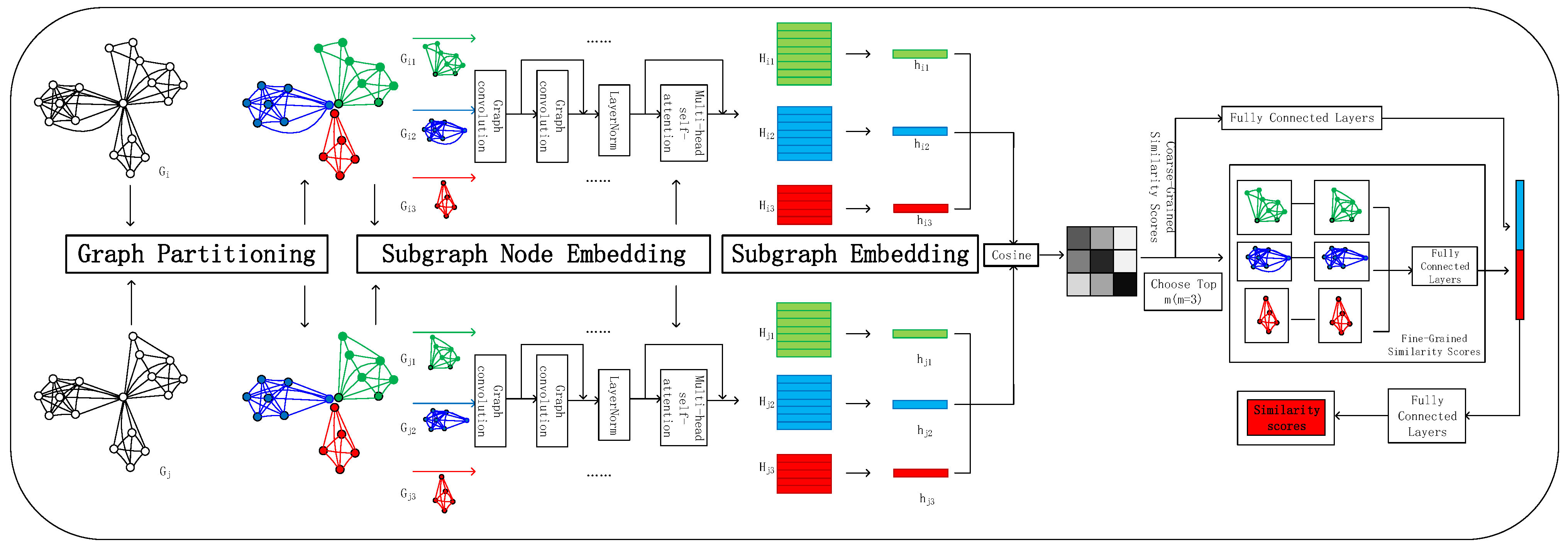
3. The Proposed Approach: APSimGNN

3.1. Problem Definition

We defined an undirected and unweighted graph G = {V, E, A}, where A represents the adjacency matrix of G; E represents a set of edges; and V denotes a set of nodes {v₁, v₂, …, v_n} with |V| = n. Each node is represented by $h^{(0)}\in R^D$, where D denotes the dimension of node feature vectors. H⁽⁰⁾ represents feature matrix. The objective was to create a neural network-based function adopting two graphs G{V_i, E_i, A_i} and G{V_j, E_j, A_j} as the input for determining the similarity score S_ij.

3.2. Graph Partitioning

The majority of the neural-network-based graph similarity computation models utilized the mechanisms for generating both the node-level and graph-level embeddings, combining the coarse-grained graph-level interactions with the fine-grained node-level comparisons to calculate the similarity scores between graph pairs. However, there can be several limitations for them when analyzing the graphs exhibiting high node count: (1) the representation of the entire graph using only graph-level embeddings is limited, potentially leading to the loss of local structural features, and (2) the high number of nodes results in significant computational costs for the node-level comparisons, with the matching of distant nodes introducing additional noise.

To address these limitations and capture the local structural features of large graphs more accurately, reference [16] employed the fluid community algorithm (FluidC) to partition the graph into k subgraphs, consisting of the following three main steps.

Step 1: Randomly select k nodes as the initial nodes for the k subgraphs, with each subgraph initially having a density of one.

Step 2: Randomly iterate through all the nodes and assign them and their neighboring nodes to a subgraph based on their current subgraph membership. The subgraph density is updated to the reciprocal of the node count. The node-assignment rule involves calculating the sum of the density products of the node and its neighboring nodes with each subgraph, selecting the subgraph with the highest sum, and assigning the node to that subgraph.

Step 3: Repeat step 2 until all nodes have completed partitioning.

The FluidC algorithm for large graph segmentation can be both simple and efficient, while it also has the following shortcomings:

(1) The FluidC algorithm falling under the edge-cutting class of graph-partitioning algorithms has little impact on the original graph data when partitioning low-level nodes in a large image. However, partitioning the high-level nodes results in a significant loss of edge information, disrupts the structure of the original graph data, and consequently affects the accuracy of subsequent similarity computations.

(2) The FluidC algorithm randomly selects k nodes from the graph data as the initial nodes for k subgraphs. If these initial nodes are too concentrated, a large number of zero values are generated during subsequent node-partitioning calculations, thereby reducing the efficiency of the algorithm and compromising the quality of subgraph partitioning. Moreover, different initial nodes may result in varying partitions, leading to inconsistent similarity calculation results.

To address these shortcomings, this study proposed the AFluidC algorithm for optimization. The core idea was to divide the high-level nodes in the graph data into k child nodes (where k is the number of subgraphs) and then assign these child nodes to subgraphs along with other nodes. The algorithm set a reasonable distance for the initial nodes, thereby ensuring that the distance between any two nodes was greater than 1/k. The specific details of the algorithm are as follows.

(1) The node classification involved traversing the edges in a graph and counting the degree of each node. If the degree exceeded 2/3 of the total nodes, it was classified as a high-degree node; otherwise, it was classified as a low-degree node.

(2) The high-degree node processing involved several steps depending on the presence of high-degree nodes in the input graph pair. If neither graph contained high-degree nodes, k initial nodes were selected according to the distance requirements between them. If only one graph had high-degree nodes, the graphs could be dissimilar, and the partitioning step could be skipped, resulting in a similarity score of zero. If both graphs had high-degree nodes, they could follow the following steps: (1) Split each high-degree node into k child nodes and process all edges of the original high-degree node. (2) Select an edge to connect to a child node and include this child node, the edge, another node connected to the edge, and all associated edges in subgraph 1. The remaining edges were processed as follows: if an edge connected to a child node already marked for a subgraph partition, the child node was then connected, and the connected nodes and edges were divided to the corresponding subgraphs. If an edge did not connect to any labeled child nodes, an unlabeled child node was selected and connected to that edge. The edge was marked with the child nodes as part of a new subgraph.

(3) The algorithm converged once all the edges of the high-degree nodes were processed, and the edges and nodes could be successfully partitioned.

An example illustrating the process of dividing a graph with a high-degree node was presented. Figure 1a depicts the input graph G that contained 18 nodes and was partitioned into the k = 3 subgraphs. The central node had a degree of 17, exceeding 2/3 of the total number of nodes, thus qualifying it as a high-degree node. Following the described algorithm, the nodes in the graph were partitioned into three subgraphs, as illustrated in Figure 1.

3.3. Subgraph Node Embedding

During the graph-partitioning phase, two sets of subgraphs were generated, including {G_i1, G_i2, …G_ik} and {G_j1, G_j2, …G_jk}. Subsequently, the node features of these subgraphs could be extracted.

Accurate node embedding is essential for improving graph similarity learning. Drawing inspiration from the NA-GSL algorithm [33], we integrated the graph convolution with a multihead graph self-attention mechanism into the node encoding to derive the embedding vector for each subgraph. Hereafter, G represents a subgraph.

The algorithm initially learned the local node embeddings using a residual graph convolution module and subsequently captured the global information through the multi-head graph self-attention mechanism for enhancing the node representation.

The ordinary graph convolutional layers aggregated the node embeddings with those of adjacent nodes and transformed the combined content through the feed-forward propagation. However, deep graph convolutional modules may have caused nodes to lose their distinctiveness. To utilize the global context and prevent excessive smoothing, residual connections were introduced between the graph convolutional layers to refine the resulting node embeddings.

$$H^{(l)}=\sigma ({\tilde{D}}^{-{\displaystyle \frac{1}{2}}}\tilde{A}{\tilde{D}}^{-{\displaystyle \frac{1}{2}}}{H}^{(l-1)}{W}_{gc}^{(l)})+H^{(l-1)},$$

(1)

where H^(l) represents the output of the l-th layer; H^(l−1) represents the input of the l-th layer; I denotes the identity matrix; W_gc is the learnable weight matrix for each graph convolution layer; σ is the nonlinear activation function; $\tilde{A}$ denotes a symmetrically normalized adjacency matrix with self-connections A + I; and $\tilde{D}$ is the diagonal degree matrix of $\tilde{A}$.

Owing to the limitations of the graph convolution in modeling the remote node relationships, the residual connections alone were insufficient for effectively learning distant nodes. Consequently, the algorithm employed a multihead graph self-attention mechanism for enhancing the node embeddings.

Given a node embedding H^(l) generated by the residual graph convolution module, the query Q^m, key K^m, and value V^m required for the graph self-attention mechanism were computed, where m denotes the self-attention matrix of the mth head.

Q^m = H^(l)W^Qm, K^m = H^(l)W^Km, V^m = H^(l)W^Vm,

(2)

where W^Qm, W^Km, and W^Vm are the learnable weight matrices for querying Q^m, key K^m, and value V^m.

The algorithm employed the multihead graph attention mechanism to generate the node embeddings while also incorporating the relative distance between nodes. By using a normalization matrix D_g to represent the shortest path distance between nodes, the quality of node embeddings was enhanced. The embedding of the mth head node in the output is represented as

$${\tilde{H}}^m=soft\max (Q^m{(K^m)}^T/\sqrt{d_k}+r{D}_g)V^m.$$

(3)

Subsequently, the m-head outputs were connected to obtain node embeddings $\tilde{H}$:

$$\tilde{H}=Concat({\tilde{H}}^1,{\tilde{H}}^2\dots ,{\tilde{H}}^m),$$

(4)

and finally, the $\tilde{H}$ was multiplied with the trainable feature matrix for dimensionality reduction to obtain the final node features $H$.

3.4. Subgraph Embedding

To generate the subgraph embeddings, the attention mechanisms were utilized to assign the weights to different nodes. The weighted sum of the node embedding vectors was then computed to represent the subgraph embeddings. The attention module in this stage emphasized the nodes that captured the global structural information of the subgraph more effectively, rather than simply averaging all the nodes or assigning the weights based on the node degrees.

The algorithm adopted the node embedding vector from the previous stage to calculate the context vector $c$, which captured the global structural properties of the subgraph:

$$c={\sigma }_1(({\displaystyle \frac{1}{n}}{\displaystyle \sum _{i=1}^n{h}_i})W_{gc}),$$

(5)

where σ is the activation function ReLU; and h_i is the embedding vector for each specific node.

$$a_i={\sigma }_2({(h_i)}^T\cdot c),$$

(6)

$$h={\displaystyle {\sum }_{i=1}^n(a_i\cdot h_i)},$$

(7)

where formula (6) calculates the attention weight a_i for each node i by multiplying the transpose of each node embedding vector $h_i$ by the context vector c, computing the inner product, and applying the sigmoid activation function. This process adjusted the context vector c and determined the attention weights. Formula (7) then computes the embedding vectors of the subgraphs by conducting the weighted sum of attention weights a_i and node embeddings $h_i$.

3.5. Graph Similarity Score Computation

The well-designed attention mechanism and node embedding should embed the graphs with similar features and structures close together in space, resulting in relatively small distances between them. To assess this, we first adopted the cosine similarity for determining the similarity between graph embedding pairs:

$$s(h_i,h_j)=\cos (h_i,h_j)={\displaystyle \frac{h_i\cdot h_j}{\left|\right|h_i\left|\right| \times \left|\right|h_j\left|\right| }},$$

(8)

where the input graphs G_i and G_j contained a total of k² subgraphs. Using formula (8), we calculated the k² similarity scores, which were then mapped to the similarity scores between the large graph pairs using a multi-layer perceptron (MLP). The calculation is as follows:

$$s(G_i,G_j)=MLP(\underset{i\prime =1,j\prime =1}{\overset{k}{\oplus }}s(h_i^{i\prime },h_j^{j\prime })),$$

(9)

But the similarity score obtained through the cosine calculations was relatively coarse. Therefore, the algorithm selected the top m pairs of subgraphs with the highest similarity for a more precise calculation.

Let the input subgraph pair be represented as $G_1$ and $G_2$, with the corresponding node sets as $V_1$ and $V_2$ and the edge sets as $E_1$ and $E_2$. First, the nodes in $G_1$ and $G_2$ interacted together. The formula for calculating the effect of node p on node q within the subgraph is as follows.

$$v_{p\to q}=MLP(h_p^{(t)}\oplus h_q^{(t)}),\forall (p,q)\in E_1\cup E_2,$$

(10)

where the $h_p^{(t)}$ denotes the node embedding of node p after the t-th iteration.

Next, we calculated the interaction between subgraphs $G_1$ and $G_2$. In this calculation, the attention mechanism was employed to assign varying weights to the nodes within the subgraph, highlighting the significance of various nodes p to q. This approach amplified the influence of similar nodes within the subgraph.

$$a_{p\to q}={\displaystyle \frac{\exp (h_p^{(t)}\cdot h_q^{(t)})}{{\displaystyle {\sum }_{p\prime }\exp (h_{p\prime }^{(t)}\cdot h_q^{(t)})}}},$$

(11)

The following formula was used to represent the interaction between nodes p and q:

$${\mu }_{p\to q}=a_{p\to q}(h_q^{(t)}-h_p^{(t)}),\forall q\in V_A^i,p\in V_B^j,or\forall p\in V_A^i,q\in V_B^j.$$

(12)

After calculating the node interactions within the subgraphs and between the subgraph pairs, the information from the t-th propagation round was merged, leading to the generation of node information for the (t + 1)-th propagation round:

$$h_q^{(t+1)}=MLP(h_q^{(t)}\oplus {\displaystyle \sum _p{v}_{p\to q}\oplus {\displaystyle \sum _{p\prime }{\mu }_{p\prime \to q}}}).$$

(13)

After T iterations, the final node embeddings represented by h^(T) were obtained. These embeddings were then aggregated using a self-attention mechanism for the generation of the subgraph-level embedding.

$$h_{agg}=ML{P}_{agg}({\displaystyle \sum _{i\in V}\sigma (ML{P}_{att}(h^{(T)}))}\cdot MLP(h^{(T)})).$$

(14)

After determining the detailed embedding vectors for the subgraphs, their similarities were measured using cosine similarity, expressed as follows:

$$s(h_{agg1},h_{agg2})=\cos (h_{agg1},h_{agg2})={\displaystyle \frac{h_{agg1}\cdot h_{agg2}}{\left|\right|h_{agg1}\left|\right|\times \left|\right|h_{agg2}\left|\right|}}.$$

(15)

The precise similarity score for the m subgraph pairs with the highest similarity scores among k² pairs can be calculated using MLP, resulting in

$$s(G_i,G_j)″=MLP(\underset{t=1}{\overset{m}{\oplus }}s(h_{aggi}^{it},h_{aggj}^{jt})).$$

(16)

Finally, the algorithm employed a multi-layer perceptron (MLP) to map the k² rough similarity and the m more accurate similarity scores to the final predicted similarity s (G_i, G_j) for the graph pair. The calculation formula is shown below:

$$s(G_i,G_j)=MLP (s(G_i,G_j)\prime \oplus s(G_i,G_j)″).$$

(17)

The process of the algorithm is shown in Figure 2.

4. Experiment

4.1. Dataset

The experimental data for the algorithm were classified into two groups: artificial and real data. The artificial data utilized the graph similarity computation dataset based on the Barabási–Albert priority attachment model (BA model), as proposed in [23]. This dataset included three subdatasets: BA-60, BA-100, and BA-200, which were named according to the average number of nodes in each graph. The real data comprised the Internet Movie Database (IMDB) [34] and its subset IMDBX [16].

Table 1. Dataset parameters.

Dataset	#Graphs	#Pairs	#Min Nodes	#Max Nodes	#Avg Nodes	#Min Edges	#Max Edges	#Avg Edges
BA-60	200	40,000	54	65	60	54	66	60
BA-100	200	40,000	96	105	100	96	107	100
BA-200	200	40,000	192	205	200	193	206	200
IMDBX	220	48,400	15	52	21	33	186	74
IMDB	1500	2,250,000	7	89	13	12	1467	66

provides essential details of these five datasets, including the dataset size (#Graphs), the number of graph pairs (#Pairs), the minimum and maximum number of nodes (#Min Nodes, #Max Nodes), the average number of nodes (#Avg Nodes), and the minimum, maximum, and average number of edges (#Min Edges, #Max Edges, #Avg Edges).

The BA dataset consisted of 200 graphs divided into two parts. Two of these were the basic graphs generated using the algorithm from [35], which simulated the skewed power-law distribution in real networks, where most nodes were low degree and only a few were high degree. The remaining 198 graphs were generated by editing these two basic graphs, resulting in a dataset that could produce more similar graphs.

The Internet Movie Database (IMDB) comprised movies, actors, producers, and related entities, with each graph representing the work of a movie actor. An edge in the graph demonstrated that two entities appeared in the same movie. Owing to the large amount of graph data in IMDB, a subset called IMDBX, matching the size of the BA dataset, was filtered for comparison. Each graph in the IMDBX contained at least 15 nodes, and the ratio of edges to nodes was less than 5. This filtering ensured a sufficient number of nodes with moderate density, making the data suitable for graph division during preprocessing.

Sixty percent of the graph pairs from each dataset were stochastically extracted as the training set, 20% were extracted for the test set, and 20% were regarded as the validation set.

Figure 3, Figure 4, Figure 5 and Figure 6 present the node degree distribution for the BA model and IMDB-X datasets. The average node count in the BA model dataset was approximately one, indicating a relatively sparse graph structure, which was well suited for the extraction of the local structural features through graph partitioning. The node degree distribution demonstrated that most of the modes presented low degrees, whereas only several nodes exhibited high degrees. These high-degree nodes were more likely to become central nodes within the subgraphs.

4.2. Ground-Truth Generation

During the generation of the BA dataset, 99 exported graphs were produced for each of the two basic graphs. These exported graphs were created through various editing operations, such as deleting or adding nodes, or removing the edges from the basic graph. The editing distance between the basic graph and each exported graph, referred to as the GED value, can be determined by recording the number and type of the editing operations.

The BA dataset contained 198 pairs of graphs, for which the similarity truth values could be determined using the aforementioned method. For the remaining graph pairs, the GED values were calculated using three classic approximation algorithms: Hungarian [36], VJ [24], and Beam [37]. The GED truth value for these pairs was taken as the minimum result obtained from these three algorithms.

For IMDB and IMDBX datasets consisting of the real data, the GED truth values were calculated using the three approximate algorithms mentioned above, with the minimum result from these algorithms being selected.

Subsequently, the calculated GED value was converted into the similarity for our model. This was achieved by normalizing the GED value using the following formula: $GED\left(G_1,G_2\right)\prime ={\displaystyle \frac{GED\left(G_1,G_2\right)}{\left(\left|G_1\right|+\left|G_2\right|\right)/2}}$, with the GED value of the graph pair divided by the average node count in the graph pair. Subsequently, the exponential function $f\left(x\right)=e^{-x}$ was adopted to map the normalized GED to a range of 0 to 1 for obtaining the true similarity. The calculation formula indicates that a smaller GED could present a higher similarity between graph pairs, resulting in a similarity score closer to 1.

4.3. Results and Analysis

4.3.1. Baseline Methods

Our baseline methods could be categorized into three types: embedding, matching, and hybrid models.

The first category comprised two embedding models: GCN Max and GCN Mean [11]. Both of the models utilized GCN to embed the graphs into vectors, with the similarity between graph pairs determined by calculating the similarity between these vectors.

The second category involved two graph-matching-based models: GSimCNN [12], which integrated the embedding with node-level comparisons of the entire graph, and GMN [13] that calculated the similarity by comparing the node information both within and between graphs.

The third category consisted of three hybrid models: SimGNN [10], NAGSim [15], and PSimGNN [16]. These models integrated both the graph-level and node-level embeddings of the input graph and combine them to represent the graph comprehensively.

4.3.2. Parameter Settings

The parameter settings for APSimGNN are as follows:

A constant encoding scheme was used for the initial nodes in the input graph.

In the graph-partitioning stage, the parameter k was set to three, with nine subgraph pairs generated from the two input graphs.

In the node-level embedding stage, the graph convolutional layers were configured to three, and the embedding size in the residual GNN was initialized to 32, with the count of the multihead attention heads initialized to eight.

In the similarity calculation stage, the top zero, three, and nine subgraph pairs with the highest similarity were extracted for the precise similarity assessment. These approaches were designated as APSimGNN-0 (only using rough cosine similarity calculation), APSimGNN-m (where m = 3 for accurate subgraph similarity calculation), and APSimGNN (where all the subgraph pairs were subjected to the accurate similarity calculation).

For the rough cosine similarity calculation results, a fully connected layer was employed for reducing the vector dimension from 9 to 8. Additionally, another fully connected layer adjusted the dimension of the fine-grained similarity calculation result vector from 3 to 8. Finally, four fully connected layers were adopted to consolidate the dimensions of the two cosine similarity vectors from 16 to 1.

Empirically, the batch size was set to 128, the optimization was performed using the Adam algorithm [24]. The iterations were 2000, and the training was stopped if the validation loss did not decrease after 100 iterations. The initial learning rate was set to 0.001, and it was halved when the loss failed to decrease after 100 iterations.

4.3.3. Evaluation Metrics

The following metrics were adopted to evaluate the similarity calculation results of all models.

(1) The run time referred to the total duration required by each method to estimate the similarity score for all graph pairs in the dataset.

(2) The MSE measured the average squared difference between the calculated similarities and true values.

(3) The Mean Absolute Error (MAE) measured the average absolute deviation between the true values and the calculated similarities.

(4) The Kendall’s rank correlation coefficient (τ) and Spearman’s rank correlation coefficient (ρ) were utilized to determine the degree of correspondence between the predicted and actual ranking results.

The smaller values for runtime, MSE, and MAE indicated better performance, whereas the larger values for the Kendall’s rank correlation coefficient (τ) and Spearman’s rank correlation coefficient (ρ) suggested that the predicted values were more closely aligned with the actual data.

4.3.4. Result Analysis

The experimental outcomes for these datasets are presented in

Table 2. Accuracy of different graph neural network models on BA datasets. The best result is indicated in bold.

Methods	BA-60				BA-100				BA-200
	MSE	MAE	ρ	τ	MSE	MAE	ρ	τ	MSE	MAE	ρ	τ
GCN-Mean [11]	0.58	5.39	0.756	0.532	1.25	9.09	0.763	0.533	2.37	12.78	0.734	0.488
GCN-Max [11]	1.37	9.14	0.746	0.523	1.20	8.54	0.761	0.530	2.28	10.76	0.749	0.516
GSimCNN [12]	0.60	5.61	0.807	0.604	0.23	3.25	0.823	0.616	0.32	3.58	0.796	0.568
GMN [13]	0.27	3.82	0.763	0.546	0.15	2.71	0.772	0.542	0.12	2.66	0.795	0.578
SimGNN [10]	0.78	6.58	0.773	0.567	0.80	6.93	0.763	0.538	0.84	6.19	0.734	0.488
NAGSim [16]	0.24	4.13	0.814	0.613	0.13	3.01	0.798	0.565	0.08	2.48	0.753	0.523
PSimGNN [17]	0.20	3.39	0.844	0.661	0.11	2.41	0.801	0.584	0.06	1.96	0.791	0.572
APSimGNN	0.18	3.32	0.859	0.632	0.09	2.21	0.832	0.613	0.05	1.88	0.821	0.596

,

Table 3. Accuracy of different graph neural network models on real datasets. The best result is indicated in bold.

Methods	IMDBX				IMDB
	MSE	MAE	ρ	τ	MSE	MAE	ρ	τ
GCN-Mean [11]	2.22	5.54	0.466	0.362	0.69	3.69	0.423	0.307
GCN-Max [11]	4.71	12.32	0.246	0.173	0.51	4.33	0.565	0.342
GSimCNN [12]	0.50	3.04	0.662	0.498	0.08	1.07	0.895	0.847
GMN [13]	0.38	2.73	0.695	0.553	0.08	0.97	0.853	0.818
SimGNN [10]	0.74	3.37	0.527	0.393	0.13	2.19	0.794	0.770
NAGSim [16]	0.45	2.57	0.683	0.457	0.11	1.36	0.832	0.792
PSimGNN [17]	0.31	2.51	0.723	0.603	0.07	0.78	0.859	0.822
APSimGNN	0.27	2.11	0.736	0.636	0.06	0.63	0.872	0.817

,

Table 4. Average running time for one pair of graphs on the BA dataset (ms).

Methods	BA-60	BA-100	BA-200
GCN-Mean [11]	256	348	408
GCN-Max [11]	284	368	452
GSimCNN [12]	100	124	224
GMN [13]	376	552	1500
SimGNN [10]	176	224	276
NAGSim [16]	147	213	319
PSimGNN [17]	624	800	1200
APSimGNN	553	616	824

and

Table 5. Impact of accurate similarity calculation on results of different number of subgraph pairs. The best result is indicated in bold.

Methods	BA-60				BA-100				BA-200
	MSE	MAE	ρ	τ	MSE	MAE	ρ	τ	MSE	MAE	ρ	τ
APSimGNN-0	0.34	4.70	0.793	0.594	0.39	3.94	0.789	0.578	0.07	3.94	0.774	0.529
APSimGNN-m	0.28	4.02	0.825	0.616	0.12	2.39	0.814	0.597	0.06	2.03	0.793	0.553
APSimGNN	0.18	3.32	0.859	0.632	0.09	2.21	0.832	0.613	0.05	1.88	0.821	0.596

, with the optimal data highlighted in bold. The tables indicate that across the datasets, the performance of GCN Max and GCN Mean was generally inferior compared to other models on most evaluation metrics. As the node count in each graph increased, the limitations of employing a single vector for representing the graph became more pronounced, leading to poor results.

Table 2 presents the performance indicators of the various algorithms on the BA dataset. The PSimGNN and APSimGNN algorithms consistently achieved the optimal or suboptimal results for most evaluation metrics across the three BA datasets, highlighting the effectiveness of incorporating subgraphs to calculate the large graph similarities. Although PSimGNN demonstrated some suboptimal performances in ranking indicators (ρ, τ) for BA-100 and BA-200 owing to the randomness in graph partitioning, the APSimGNN algorithm demonstrated a significantly improved performance. This improvement confirmed the effectiveness of optimizing the graph-partitioning stage and utilizing attention mechanisms for both node and graph embeddings. In the BA-60 and BA-100 datasets, the APSimGNN algorithm produced some results slightly below the optimal value, falling short of those achieved by PSimGNN. This is likely owing to the small number of nodes in the data graph and the limited number of height nodes. Although the graph-partitioning method used by APSimGNN performs similarly to the random partitioning method in PSimGNN, it still has significant advantages over other neural network algorithms.

Table 3 presents the performance indicators of these algorithms for the real datasets. APSimGNN achieved the best performance on the IMDBX dataset, outperforming PSimGNN in all metrics. In the IMDB dataset, some graphs were dense with a large number of edges, which obscured the clarity of the local structure. In addition, a large number of nodes in the graph are height nodes. In the case of a small k value, the APSimGNN algorithm only partitions some of these height nodes, thereby limiting the full benefits of graph partitioning. Although some indicators in the experimental results did not reach the optimal level, the algorithm still maintained suboptimal performance compared with similar algorithms.

Table 4 compares the running times of various algorithms, including the proposed APSimGNN, across three different scales of the BA datasets. The wall time required for each model to compute the similarity score for a pair of graphs was collected. All methods were randomly run 10 times. Notably, the theoretical computational costs did not always align with the actual running times. For instance, although GCN Mean and GCN Max had a theoretical computational cost of O(N), their models incorporated several layers of node embeddings to optimize performance, leading to higher actual running times. Conversely, GSimCNN theoretically requiring the O(N²) computational cost could achieve the fastest running time due to optimizations in its CNN framework.

When the number of nodes in the input graph was small, the PSimGNN and APSimGNN algorithms required additional steps for graph partitioning, leading to slightly longer running times than the other algorithms. However, as the number of nodes increased, we found that these algorithms could perform accurate similarity calculations only on smaller subgraphs; therefore, the increase in the running time was minimal. In particular, APSimGNN optimized the graph partitioning, resulting in a significant reduction in the running time compared to PSimGNN.

Table 5 compares the metrics for selecting different numbers of graph pairs for precise similarity calculation in the APSimGNN algorithm. APSimGNN-0 referred to the rough cosine similarity calculation for all subgraph pairs, APSimGNN-m indicated the precise similarity calculation for m subgraph pairs before selecting the cosine similarity values, and APSimGNN denoted the precise similarity calculation for all the subgraph pairs. The experimental data demonstrated that as the number of precisely calculated subgraph pairs increased, the algorithm incorporated more information, leading to improved performance metrics that aligned with the objectives of the algorithm.

4.3.5. Parameter Optimization

This section analyzes the effects of the subgraph partition parameter k and subgraph embedding dimension D on the performance of the APSimGNN. Figure 7 illustrates the MSE of the algorithm for various k values on the BA-60 dataset. As the number of partitioned subgraphs increased, the MSE value initially decreased and then increased. This was because few subgraphs failed to capture the local features of the graph, whereas numerous subgraphs could disrupt the overall structure. The results suggested that choosing three or four partitions was optimal. Figure 8 illustrates the impact of the subgraph embedding dimension D on the performance. However, as the embedding dimension increased, the performance improved because a larger dimension provided more capacity for representing subgraphs. However, the performance gains diminish once D exceeded a certain threshold. The results indicated that a subgraph embedding dimension of 32 yielded the best balance between algorithm performance and complexity.

5. Conclusions

This study addressed the limitations of the graph-partitioning strategy in the PSimGNN algorithm and proposed a rational improvement. We introduced an attention mechanism for the node-level and subgraph-level embeddings of subgraphs. In the similarity calculation stage, all the subgraph pairs underwent an initial rough cosine similarity calculation. Subsequently, the top m scoring subgraphs were selected for a detailed node-level similarity calculation. Finally, the multilayer perceptron (MLP) integrated these scores to determine the final large-graph similarity. The experimental results demonstrated that the proposed APSimGNN algorithm outperformed PSimGNN across various performance metrics and was more effective in handling the large-scale graph data similarity calculations.

Owing to the limitations in accurately calculating the GED value of large graphs, current algorithms rely on approximate GED values to determine the truth in the learning model. As the number of nodes increases, the accuracy of these approximation algorithms decreases. Future work will focus on extending the learned model to accommodate the larger graphs by training it exclusively on precise GED values between the partitioned subgraphs or other smaller graph datasets. This approach aims to enhance both the scalability and performance metrics of the algorithm.

References

1. Miao, F.Y.; Wang, H.Z. Method for similarity join on uncertain graph database. J. Softw. 2018, 29, 3150–3163. (In Chinese) [Google Scholar]
2. Blumenthal, D.B.; Boria, N.; Gamper, J.; Bougleux, S.; Brun, L. Comparing heuristics for graph edit distance computation. VLDB J. 2020, 29, 419–458. [Google Scholar] [CrossRef]
3. Chang, L.; Feng, X.; Lin, X.; Qin, L.; Zhang, W.; Ouyang, D. Speeding up GED verification for graph similarity search. In Proceedings of the 2020 IEEE 36th International Conference on Data Engineering (ICDE), Dallas, TX, USA, 20–24 April 2020. [Google Scholar]
4. Riesen, K.; Ferrer, M.; Bunke, H. Approximate graph edit distance in quadratic time. IEEE/ACM Trans. Comput. Biol. Bioinform. 2015, 17, 483–494. [Google Scholar] [CrossRef] [PubMed]
5. Bunke, H. On a relation between graph edit distance and maximum common subgraph. Pattern Recognit. Lett. 1997, 18, 689–694. [Google Scholar] [CrossRef]
6. Blumenthal, D.B.; Gamper, J. On the exact computation of the graph edit distance. Pattern Recognit. Lett. 2020, 134, 46–57. [Google Scholar] [CrossRef]
7. Kim, J.; Choi, D.H.; Li, C. Inves: Incremental Partitioning-Based Verification for Graph Similarity Search. EDBT 2019. [Google Scholar] [CrossRef]
8. Liang, Y.; Zhao, P. Similarity search in graph databases: A multi-layered indexing approach. In Proceedings of the 2017 IEEE 33rd International Conference on Data Engineering (ICDE), San Diego, CA, USA, 19–22 April 2017. [Google Scholar]
9. Blumenthal, D.B.; Gamper, J. Improved lower bounds for graph edit distance. IEEE Trans. Knowl. Data Eng. 2017, 30, 503–516. [Google Scholar] [CrossRef]
10. Bai, Y.; Ding, H.; Bian, S.; Chen, T.; Sun, Y.; Wang, W. Simgnn: A neural network approach to fast graph similarity computation. In Proceedings of the Twelfth ACM International Conference on Web Search and Data Mining (WSDM’19), New York, NY, USA, 11–15 February 2019. [Google Scholar]
11. Defferrard, M.; Bresson, X.; Vandergheynst, P. Convolutional neural networks on graphs with fast localized spectral filtering. Adv. Neural Inf. Process. Syst. 2016, 29, 3844–3852. [Google Scholar]
12. Bai, Y.; Ding, H.; Sun, Y.; Wang, W. Convolutional set matching for graph similarity. arXiv 2018, arXiv:1810.10866. [Google Scholar]
13. Li, Y.; Gu, C.; Dullien, T.; Vinyals, O.; Kohli, P. Graph matching networks for learning the similarity of graph structured objects. In Proceedings of the 36th International Conference on Machine Learning, PMLR, Long Beach, CA, USA, 9–15 June 2019; Volume 97, pp. 3835–3845. [Google Scholar]
14. Qin, Z.; Bai, Y.; Sun, Y. GHashing: Semantic graph hashing for approximate similarity search in graph databases. In Proceedings of the 26th ACM SIGKDD International Conference on Knowledge Discovery & Data Mining, New York, NY, USA, 6–10 July 2020. [Google Scholar]
15. Hou, Y.; Ning, B.; Hai, C.; Zhou, X.; Yang, C.; Li, G. NAGSim: A Graph Similarity Model Based on Graph Neural NetWorks and Attention Mechanism. J. Chin. Comput. Syst. 2023, 44, 1665–1671. [Google Scholar]
16. Xu, H.; Duan, Z.; Wang, Y.; Feng, J.; Chen, R.; Zhang, Q.; Xu, Z. Graph partitioning and graph neural network based hierarchical graph matching for graph similarity computation. Neurocomputing 2021, 439, 348–362. [Google Scholar] [CrossRef]
17. Parés, F.; Gasulla, D.G.; Vilalta, A.; Moreno, J.; Ayguadé, E.; Labarta, J.; Cortés, U.; Suzumura, T. Fluid communities: A competitive, scalable and diverse community detection algorithm. In Complex Networks & Their Applications VI. COMPLEX NETWORKS 2017; Cherifi, C., Cherifi, H., Karsai, M., Musolesi, M., Eds.; Studies in Computational Intelligence; Springer: Cham, Switzerland, 2018; Volume 689, pp. 229–240. [Google Scholar]
18. Buluç, A.; Meyerhenke, H.; Safro, I.; Sanders, P.; Schulz, C. Recent advances in graph partitioning. In Algorithm Engineering. Lecture Notes in Computer Science; Kliemann, L., Sanders, P., Eds.; Springer: Cham, Switzerland, 2016; Volume 9220, pp. 117–158. [Google Scholar]
19. Kaburlasos, V.G.; Moussiades, L.; Vakali, A. Fuzzy lattice reasoning (FLR) type neural computation for weighted graph partitioning. Neurocomputing 2009, 72, 2121–2133. [Google Scholar] [CrossRef]
20. Adoni, H.W.Y.; Nahhal, T.; Krichen, M.; Aghezzaf, B.; Elbyed, A. A survey of current challenges in partitioning and processing of graph-structured data in parallel and distributed systems. Distrib. Parallel. Dat. 2020, 38, 495–530. [Google Scholar] [CrossRef]
21. Kipf, T.N.; Welling, M. Semi-supervised classification with graph convolutional networks. arXiv 2016, arXiv:1609.02907. [Google Scholar]
22. Ma, Y.; Wang, S.; Aggarwal, C.C.; Tang, J. Graph convolutional networks with eigenpooling. In Proceedings of the 25th ACM SIGKDD International Conference on Knowledge Discovery & Data Mining (KDD’19), New York, NY, USA, 4–8 August 2019. [Google Scholar]
23. Veličković, P.; Cucurull, G.; Casanova, A.; Romero, A.; Liò, P.; Bengio, Y. Graph attention networks. arXiv 2017, arXiv:1710.10903. [Google Scholar]
24. Xu, K.; Hu, W.; Leskovec, J.; Jegelka, S. How Powerful are Graph Neural Networks? arXiv 2018, arXiv:1810.00826. [Google Scholar]
25. Qiu, J.; Chen, Q.; Dong, Y.; Zhang, J.; Yang, H.; Ding, M.; Wang, K.; Tang, J. Gcc: Graph contrastive coding for graph neural network pre-training. In Proceedings of the 26th ACM SIGKDD International Conference on Knowledge Discovery & Data Mining (KDD’20), New York, NY, USA, 6–10 July 2020. [Google Scholar]
26. Xu, K.; Li, C.; Tian, Y.; Sonobe, T.; Kawarabayashi, K.; Jegelka, S. Representation learning on graphs with Jumping knowledge networks. In Proceedings of the 35th International Conference on Machine Learning, PMLR, Stockholm, Sweden, 10–15 July 2018; Volume 80, pp. 5453–5462. [Google Scholar]
27. Cai, L.; Li, J.; Wang, J.; Ji, S. Line graph neural networks for link prediction. IEEE Trans. Pattern Anal. Mach. Intell. 2021, 44, 5103–5113. [Google Scholar] [CrossRef]
28. Zhang, M.; Chen, Y. Link prediction based on graph neural networks. Adv. Neural Inf. Process. Syst. 2018. [Google Scholar] [CrossRef]
29. Liu, J.; Shang, X.; Song, L.; Tan, Y. Progress of Graph Neural Networks on Complex Graph Mining. J. Softw. 2022, 33, 3582–3618. (In Chinese) [Google Scholar]
30. Bruna, J.; Zaremba, W.; Szlam, A.; LeCun, Y. Spectral networks and locally connected networks on graphs. arXiv 2013, arXiv:1312.6203. [Google Scholar]
31. Bai, Y.; Ding, H.; Gu, K.; Sun, Y.; Wang, W. Learning-based efficient graph similarity computation via multi-scale convolutional set matching. Proc. AAAI Conf. Artif. Intell. 2020, 34, 3219–3226. [Google Scholar] [CrossRef]
32. Doan, K.D.; Manchanda, S.; Mahapatra, S.; Reddy, C.K. Interpretable graph similarity computation via differentiable optimal alignment of node embeddings. In Proceedings of the 44th International ACM SIGIR Conference on Research and Development in Information Retrieval (SIGIR’21), New York, NY, USA, 11–15 July 2021. [Google Scholar]
33. Tan, W.; Gao, X.; Li, Y.; Wen, G.; Cao, P.; Yang, J.; Li, W.; Zaiane, O.R. Exploring attention mechanism for graph similarity learning. Knowl.-Based Syst. 2023, 276, 110739. [Google Scholar] [CrossRef]
34. Yanardag, P.; Vishwanathan, S. Deep graph kernels. In Proceedings of the 21th ACM SIGKDD International Conference on Knowledge Discovery and Data Mining (KDD’15), New York, NY, USA, 10–13 August 2015. [Google Scholar]
35. Jain, N.; Liao, G.; Willke, T.L. Graphbuilder: Scalable graph etl Graphbuilder: Scalable graph etl framework. In First International Workshop on Graph Data Management Experiences and Systems (GRADES’13); ACM: New York, NY, USA, 2013. [Google Scholar]
36. Vaswani, A.; Shazeer, N.; Parmar, N.; Uszkoreit, J.; Jone, L.; Gomez, A.N.; Kaiser, L.; Polosukhin, I. Attention is all you need. Adv. Neural Inf. Process. Syst. 2017, 30, 1–10. [Google Scholar]
37. Zeng, Z.; Tung, A.K.H.; Wang, J.; Feng, J.; Zhou, L. Comparing stars: On approximating graph edit distance. Proc. VLDB Endow. 2009, 2, 25–36. [Google Scholar] [CrossRef]
Figure 1. (ai) represents the process of partitioning a graph with high-degree nodes in the input graph.
Electronics 13 03794 g001
Figure 2. General architecture and workflow of APSimGNN.
Electronics 13 03794 g002
Figure 3. Nodes Degree Distribution of BA-60.
Electronics 13 03794 g003
Figure 4. Nodes Degree Distribution of BA-100.
Electronics 13 03794 g004
Figure 5. Nodes Degree Distribution of BA-200.
Electronics 13 03794 g005
Figure 6. Nodes Degree Distribution of IMDB-X.
Electronics 13 03794 g006
Figure 7. Relationship between subgraph partition number k and MSE.
Electronics 13 03794 g007
Figure 8. Relationship between subgraph embedding dimension D and MSE.
Electronics 13 03794 g008