An Efficient Maximum Entropy Approach with Consensus Constraints for Robust Geometric Fitting

Abstract

Robust geometric fitting is one of the crucial and fundamental problems in computer vision and pattern recognition. While random sampling and consensus maximization have been popular strategies for robust fitting, finding a balance between optimization quality and computational efficiency remains a persistent obstacle. In this paper, we adopt an optimization perspective and introduce a novel maximum consensus robust fitting algorithm that incorporates the maximum entropy framework into the consensus maximization problem. Specifically, we incorporate the probability distribution of inliers calculated using maximum entropy with consensus constraints. Furthermore, we introduce an improved relaxed and accelerated alternating direction method of multipliers (R-A-ADMMs) strategy tailored to our framework, facilitating an efficient solution to the optimization problem. Our proposed algorithm demonstrates superior performance compared to state-of-the-art methods on both synthetic and contaminated real datasets, particularly when dealing with contaminated datasets containing a high proportion of outliers.

1. Introduction

Fitting models that are capable of handling noise and outliers find it challenging when dealing with real-world data. In the field of 3D vision, the robust fitting of models is a crucial issue when it comes to establishing correspondences between feature points in images. This technique has a wide range of applications in various domains, such as multi-model fitting [1,2], image stitching [3], wide baseline matching [4,5,6], multi-view geometry [7,8], simultaneous localization and mapping (SLAM) [9], object detection and segmentation [10,11], among others [12,13]. The common practice in this context has been the adoption of the well-established random sample consensus (RANSAC) algorithm [14,15,16,17,18]. Nevertheless, RANSAC cannot guarantee optimal solutions, and its efficiency decreases exponentially with respect to increasing outliers. Despite the significant body of research published in the last couple of decades aimed at improving the primitive RANSAC algorithm to accomplish a better balance between efficiency and accuracy [14,19,20,21], from an application standpoint, these methods have not yet overcome the limitations of RANSAC.

The consensus maximization framework is a widely used approach for performing deterministic searches in robust fitting problems. Specifically, we consider the dataset ${\mathcal{X}}_{\mathcal{E}}=\left\{{\mathcal{I}}_{\mathcal{E}},\mathcal{O}\right\}$ of size L, where ${\mathcal{I}}_{\mathcal{E}}={\left\{{\mathbf{x}}_i+{ϵ}_i,y_i\right\}}_{i=1}^N$ denotes the set of inlier points, $\mathcal{O}={\left\{{\mathbf{x}}_i,y_i\right\}}_{i=N+1}^L$ denotes the set of outlier points, and ${ϵ}_i$ represents additive noise that affects inlier points. Here, ${\mathbf{x}}_i,{ϵ}_i\left(i=1,\cdots ,L\right)\in {\mathbb{R}}^D$, $y_i\in \mathbb{R}$. The differentiation between outlier points and additive noise resides in the discernible dissimilarities demonstrated by outlier points in contrast to inliers. Specifically, outlier points manifest considerably greater dissimilarity compared to inlier points affected by additive noise. In Figure 1a,b, two-dimensional representation showcases the generated sample data portraying balanced and unbalanced distributions, respectively. The consensus maximization framework aims to identify the model comprising the potential topological structure encompassing the largest quantity of inliers.

The primary objective of the consensus maximization algorithm is to ascertain the most extensive consensus set by resolving an optimization problem aimed at maximizing the count of inliers. Alternatively expressed, the model’s objective is to achieve fitting by parameterizing it with $\mathit{\theta }\in {\mathbb{R}}^D$, aligning it as closely as possible with a substantial portion of the input data while maximizing the defined consensus of $\mathit{\theta }$, represented as

$$\Psi \left(\mathit{\theta }\right)=\sum _{i=1}^N\mathbb{I}\left(\left|{\mathbf{x}}_i^T\mathit{\theta }-y_j\right|\le \delta \right).$$

(1)

Here, $\mathbb{I}$ denotes the indicator function, returning 1 if its input predicate is true and 0 otherwise. The differentiation between inliers and outliers is established by comparing a residual with the predefined threshold $\delta$.

Primitive strategies for maximizing a consensus function (1) have been developed to achieve globally optimal solutions [22,23,24,25]. However, due to the fundamental intractability of maximum consensus estimation, obtaining the global optimum can only be accomplished through an exhaustive search, which is only applicable to problems with a small number of measurements and/or models of low dimensionality. In recent years, increasing attention has been devoted to locally convergent algorithms, which provide deterministically approximate solutions that lie between randomized algorithms and globally optimal algorithms [26,27,28,29,30,31]. While these methods alleviate the efficiency problem, they are still susceptible to being trapped in sensitive local optima due to the presence of uncertainties in the contaminated data.

This paper presents a novel approach for robust maximum consensus fitting, which is both deterministic and approximate. It aims to mitigate the influence of outliers, which often introduce misleading results during the optimization process. Our proposed method, which is called maximum entropy with consensus constraints (MECCs), as shown in Figure 2, is inspired by the maximum entropy strategy, which is a technique that can learn a probability distribution over a given dataset. By incorporating consensus maximization constraints into this framework, we can obtain the probability distribution of inliers, enabling us to better distinguish between inliers and outliers. Moreover, within our framework, we enhance the relaxed and accelerated alternating direction method of multipliers strategy (R-A-ADMM) [32] by employing the maximization-minimization method. This augmentation is aimed at obtaining a suboptimal value more efficiently for the proposed optimization problem.

In summary, the main contributions of the current study are the following:

• Maximum entropy with consensus constraints (MECC): By proposing a novel approach, MECCs, which integrates the maximum entropy strategy with consensus maximization constraints to effectively distinguish between inliers and outliers, enhances robustness in maximum consensus fitting.
• Enhanced optimization method: Developing an improved version of the relaxed and accelerated alternating direction method of multipliers (R-A-ADMMs) within our framework enables the attainment of a suboptimal solution for the proposed optimization problem.
• Empirical validation and performance efficiency: We performed experimental evaluations on both synthetic and real contaminated datasets to validate the proposed method alongside current state-of-the-art techniques in geometric accuracy and robustness, particularly in high outlier scenarios, despite a modest increase in computational cost.

The remainder of this paper is structured as follows. In Section 2, we provide a brief overview of related work and introduce the formulation of the maximum consensus problem. In Section 3.1, we present the framework of our proposed MECCs method. Section 3.2 details the optimization procedure. In Section 3.3, we demonstrate how our proposed framework can be used to estimate the fundamental matrix and homography transformations. In Section 4, we report the experimental results obtained using synthetic and real datasets. Finally, we conclude our work in Section 5.

2. Related Work and Problem Formulation

In this section, we summarize the work closely related to our study to provide context. Additionally, we outline relevant definitions and formulations for the geometric model fitting problem.

2.1. Related Work

Given the practical need for both robustness and efficiency in geometric model fitting, the random sampling methodology has remained the predominant approach. Numerous innovations have emerged over the past few decades to enhance the original RANSAC algorithm [15], focusing on both efficiency and accuracy. In order to accelerate the process, various efficient sampling techniques have been introduced, leveraging the prior information available in feature correspondences. For instance, NAPSAC [33] and GroupSAC [34] utilize spatial coherence, whereas EVSAC [35] and PROSAC [21] make use of matching scores as priors.

In terms of improving estimation accuracy, methods such as MLESAC [36] and MAPSAC [37] evaluate model quality using maximum likelihood processes. LO-RANSAC [14,16] performs local optimizations to refine the best model identified so far. More recently, GC-RANSAC [38] incorporates a graph-cut algorithm in the local optimization step, resulting in more accurate geometric model estimates. Additionally, MAGSAC [39] and MAGSAC++ [19] address the challenge of eliminating the need for a predefined inlier-outlier threshold, which is a critical yet challenging aspect to adjust in practice. The latest RANSAC-type algorithm, VSAC [40], introduces the concept of independent inliers to enhance its effectiveness in managing dominant planes and enables the accurate rejection of incorrect models without false positives.

From another perspective, a significant body of deterministic search algorithms has emerged, adopting an optimization-based formulation. The primary objective, known as consensus maximization, evolved from the model quality evaluation strategy of RANSAC. While RANSAC operates as a stochastic solver without guarantees of solution quality, especially when outliers exceed inliers, these deterministic methods seek global optimality. Various algorithms have been developed to achieve globally optimal solutions using techniques such as branch-and-bound [23,25,41], tree search [42,43], and enumeration [22,24], as shown in

Table 1. Summary of work related to the geometric model fitting problem.

Category	Research Study	Methodology	Key Aspects & Limitations
RANSAC-based	GC-RANSAC [38]	A hybrid method utilizing the graph-cut algorithm	This method improves inlier detection to refine the geometric model fitting, but it introduces significant computational overhead.
	MAGSAC++ [19]	A combined progressive NAPSAC method with a novel class of M-estimators	This method improves geometric model fitting accuracy by using a new model quality to reject outliers but is sensitive to parameter settings and data distribution.
	VSAC [40]	A dominant plane-handling method featuring a novel concept of independent inliers	This method leverages independent inliers for accurate model rejection and better handling of dominant planes but suffers from the limitations of RANSAC in terms of reduced accuracy and efficiency with high outlier ratios.
Optimization-based	GORE [44]	An outlier removal method using MILP in an iterative process	This method uses MILP to iteratively identify and remove outliers. However, its efficiency is significantly reduced due to the repeated application of consensus maximization after each removal.
	BCD-L1 [45]	A method utilizing a block co-ordinate descent framework	A method using block co-ordinate descent ensures finite iteration convergence to a local minimizer but is vulnerable to sensitive local optima due to data uncertainties.
	EAS [30]	A method incorporating a deterministic annealing approach	A method leveraging deterministic annealing handles the nonconvexity of truncated losses and reduces the risk of local optima but relies heavily on singular value decomposition, yielding only approximate suboptimal solutions.
	MECC (Ours)	A consensus maximization method incorporating a maximum consensus framework	This method employs an enhanced R-A-ADMM solver within the maximum entropy framework and consensus maximization constraints to effectively differentiate between inliers and outliers, thereby improving robustness in maximum consensus fitting.

.

Recent advancements focus on optimizing the more robust maximum consensus objective. For instance, GORE [44] employs a mixed integer linear programming technique for outlier removal to mitigate their negative impact, and BCD-L1 [45] utilizes a block co-ordinate descent framework to enhance robustness against outlier-induced errors, ensuring convergence within finite iterations and with a restricted local minimizer. The most recent and closely related optimization-based method to ours, EAS [30], integrates a deterministic annealing approach rooted in the maximum entropy principle to achieve more accurate local optima.

2.2. Problem Formulation

Maximizing the consensus function (1) can be viewed as a constrained optimization problem, intending to maximize the consensus set $\mathcal{I}={\left\{{\mathbf{x}}_i,y_i\right\}}_{i=1}^N$ within the domain ${\mathcal{X}}_{\mathcal{E}}$:

$$\begin{array}{cccc}\hfill & \underset{\mathit{\theta },\mathcal{I}\subseteq \mathcal{X}}{\mathrm{maximize}}\hfill & \hfill & \left|\mathcal{I}\right|\hfill \\ \hfill & \mathrm{subject}\mathrm{to}\hfill & \hfill & \left|{\mathbf{x}}_i^T\mathit{\theta }-y_i\right|\le \delta ,\forall \left\{{\mathbf{x}}_i,y_i\right\}\in \mathcal{I}.\hfill \end{array}$$

(2)

where $\delta \ge 0$ refers to the threshold used to determine whether a given data point is an inlier or an outlier. The solution, denoted as ${\mathcal{I}}^{\ast }$, corresponds to the maximum consensus set of size $\left|{\mathcal{I}}^{\ast }\right|$.

Instead of focusing on the problem (2), recent research on approximate and deterministic methods has shifted its focus to the complementary problem, where a slack variable $\mathbf{s}={\left[s_1,\cdots ,s_L\right]}^T\in {\mathbb{R}}^L$ is introduced as follows:

$$\begin{array}{cccc}\hfill & \underset{\mathit{\theta },\mathbf{s}}{\mathrm{maximize}}\hfill & \hfill & L-{\parallel \mathbf{s}\parallel }_0\hfill \\ \hfill & \mathrm{subject}\mathrm{to}\hfill & \hfill & \left|{\mathbf{x}}_i^T\mathit{\theta }-y_i\right|\le \delta +s_i,s_i\ge 0.\hfill \end{array}$$

(3)

where ${\parallel \mathbf{s}\parallel }_0$ is the ${\mathsf{\ell }}_0$ norm, which denotes the number of nonzero elements in $\mathbf{s}$. Furthermore, an alternative formulation of (3) can be expressed as follows:

$$\begin{array}{cccc}\hfill & \underset{\mathit{\theta },\mathbf{s}}{\mathrm{minimize}}\hfill & \hfill & {\parallel \mathbf{s}\parallel }_0\hfill \\ \hfill & \mathrm{subject}\mathrm{to}\hfill & \hfill & \left|{\mathbf{x}}_i^T\mathit{\theta }-y_i\right|\le \delta +s_i,s_i\ge 0.\hfill \end{array}$$

(4)

From an intuitive standpoint, $s_i$ should hold a nonzero value if the i-th datum is deemed an outlier concerning $\mathit{\theta }$. Conversely, if the i-th datum is deemed an inlier with respect to $\mathit{\theta }$, the value of $s_i$ is zero. Consequently, the maximization problem related to the consensus set transforms into a sparse optimization problem in relation to the slack variable $\mathbf{s}$.

Moreover, we can represent the inequality constraint of (4) as a pair of linear inequality constraints, which can be detailed as follows:

$${\mathbf{x}}_i^T\mathit{\theta }-y_i\le \delta +s_i\mathrm{and}-{\mathbf{x}}_i^T\mathit{\theta }+y_i\le \delta +s_i$$

(5)

Denote $\mathbf{X}={\left[{\mathbf{X}}_1^T,\cdots ,{\mathbf{X}}_L^T\right]}^T\in {\mathbb{R}}^{2L\times D}$ and $\mathbf{y}={\left[{\mathbf{y}}_1^T,\cdots ,{\mathbf{y}}_L^T\right]}^T\in {\mathbb{R}}^{2L}$ where ${\mathbf{X}}_i={\left[{\mathbf{x}}_i,-{\mathbf{x}}_i\right]}^T$ and ${\mathbf{y}}_i={\left[y_i,-y_i\right]}^T$. Then, Equation (4) can be generalized as [45]

$$\begin{array}{cccc}\hfill & \underset{\mathit{\theta },\mathbf{s}}{\mathrm{minimize}}\hfill & \hfill & {\parallel \mathbf{s}\parallel }_0\hfill \\ \hfill & \mathrm{subject}\mathrm{to}\hfill & \hfill & \mathbf{X}\mathit{\theta }-\mathbf{y}\le (\delta {\mathbf{1}}_L+\mathbf{s})\otimes {\mathbf{1}}_{\kappa },\mathbf{s}\ge \mathbf{0}.\hfill \end{array}$$

(6)

where ⊗ indicates the Kronecker product operator, and the positive integer $\kappa$ is a parameter that can be adjusted to suit the specific requirements of the given application. For instance, when addressing the robust linear regression problem, $\kappa$ is typically set to 2, while for the quasi-convex geometric residual model, $\kappa$ is set to 4 [46].

Equation (6) is difficult to solve tractably, and various strategies have been proposed to efficiently find a locally optimal solution. For example, GORE [44] employed mixed integer linear programming (MILP) for outlier removal in their work, and BCD-L1 [45] was proposed as a solution based on proximal block co-ordinate descent (BCD) frameworks. More recently, EAS [30] combined the deterministic annealing method with a linear assignment problem to obtain relatively exact results. Instead of using ${\mathsf{\ell }}_0$ norm, an alternative approach involves reformulating the objective as a convex but nonsmooth function based on the ${\mathsf{\ell }}_1$ norm. This reformulation can be expressed as follows:

$$\begin{array}{cccc}\hfill & \underset{\mathit{\theta },\mathbf{s}}{\mathrm{minimize}}\hfill & \hfill & {\parallel \mathbf{s}\parallel }_1\hfill \\ \hfill & \mathrm{subject}\mathrm{to}\hfill & \hfill & \mathbf{X}\mathit{\theta }-\mathbf{y}\le (\delta {\mathbf{1}}_L+\mathbf{s})\otimes {\mathbf{1}}_{\kappa },\mathbf{s}\ge \mathbf{0}.\hfill \end{array}$$

(7)

which can be solved through either the duality approach [47] or the alternating direction method of multipliers (ADMMs) with reduced dimensions [45].

The performance efficacy of current robust methods is constrained by their susceptibility to tentative inliers originating from outlier structures. This limitation arises due to the insufficient credibility achieved when employing the consensus maximization framework in isolation, particularly in scenarios where the number of outliers exceeds that of the inliers. In order to mitigate the problem of inconsistent inliers, we integrated the entropy maximum and consensus maximization framework to allow our method to adaptively allocate more focus to data points with more probability of being inliers.

3. Proposed Methodology

3.1. Entropy Maximum Strategy

By introducing a random variable, $Z={\sum }_{i=1}^L{Z}_i$, over a range, $\mathcal{X}=\left\{0,1,\cdots ,L\right\}$, we establish a representation for the number of inliers among the data points, where $Z_i$ denotes the inlier/outlier state of the i-th data point, taking values from the set ${\mathcal{X}}_i=\left\{0,1\right\}$. Specifically, we define a sample space $\Omega =\left\{I,O\right\}$, where I represents the state of being an inlier, and O represents the state of being an outlier. Consequently, each data point’s binary value is denoted as follows:

$$z_i=\left\{\begin{array}{cc}0,\hfill & \mathrm{if}{s}_i>0\hfill \\ 1\hfill & \mathrm{otherwise}\hfill \end{array}\right.$$

(8)

From an intuitive perspective, the assignment of $z_i=1$ signifies the i-th datum as an inlier; otherwise, it designates it as an outlier. Based on the definition of Equation (8), we observe that $Z_i=z_i$ if and only if the outcome of the random experiment is I or O. Hence, we can define the probability of the i-th point being an inlier and an outlier as follows:

$$\mathbb{P}\left(Z_i=\left(z_i=1\right)\right)=\mathbb{P}\left\{Z_i\left(I\right)=\left(z_i=1\right)\right\}=p_i$$

(9)

$$\mathbb{P}\left(Z_i=\left(z_i=0\right)\right)=\mathbb{P}\left\{Z_i\left(O\right)=\left(z_i=0\right)\right\}=1-p_i$$

(10)

In contrast to the conventional objective of minimizing the number of nonzero elements in $\mathit{s}$, we now propose the incorporation of $\mathbf{p}$ into Equation (7):

$$\begin{array}{cccc}\hfill & \underset{\mathit{\theta },\mathbf{s},\mathbf{p}}{\mathrm{minimize}}\hfill & \hfill & \parallel {\mathbf{p}}^T{·\mathbf{s}\parallel }_1\hfill \\ \hfill & \mathrm{subject}\mathrm{to}\hfill & \hfill & \mathbf{X}\mathit{\theta }-\mathbf{y}\le (\delta {\mathbf{1}}_L+\mathbf{s})\otimes {\mathbf{1}}_{\kappa },\mathbf{s}\ge \mathbf{0}.\hfill \end{array}$$

(11)

where $\mathbf{p}={[p_1,\cdots ,p_L]}^T\in {\mathbb{R}}^L$ is defined. By embracing this configuration, the model will prioritize data points with higher probabilities of being inliers. This departure from the characteristics of Equation (7) aims to minimize the slack variable $s_i$ associated with data points having higher probabilities, striving to approach zero as closely as is feasible. This adjustment serves to diminish the impact of outliers on the model. Importantly, when optimizing $\mathbf{p}$ while holding $\mathbf{b}$ and $\mathit{\theta }$ constant, Equation (11) simplifies into a straightforward linear assignment problem.

In order to address this issue, we put forth the integration of the maximum entropy strategy, positing an assumption that favors the maximization of entropy for optimization preference:

$$\begin{array}{cccc}\hfill & \underset{\mathbf{p}}{\mathrm{maximize}}\hfill & \hfill & -\sum _{i=1}^L\left[p_{i}log{p}_i+\left(1-p_i\right)log\left(1-p_i\right)\right]\hfill \\ \hfill & \mathrm{subject}\mathrm{to}\hfill & \hfill & {\mathbb{E}}_{\mathbf{p}}\left[Z\right]=\left|{\mathcal{I}}^{\ast }\right|\hfill \end{array}$$

(12)

where $\left|{\mathcal{I}}^{\ast }\right|$ is the maximum consensus size of the optimal value in (2) as a reminder, and ${\mathbb{E}}_{\mathbf{p}}\left[Z\right]={\sum }_{i=1}^L{p}_i$ represent the expectation of Z. Furthermore, the Lagrangian reformulation of this optimization of Equation (12) is as follows:

$$\begin{array}{cccc}\hfill & \underset{\mathbf{p}}{\mathrm{minimize}}\hfill & \hfill & \sum _{i=1}^L\left[p_{i}log{p}_i+\left(1-p_i\right)log\left(1-p_i\right)\right]\hfill \\ \hfill & \hfill & & +\lambda \left|{\mathbb{E}}_{\mathbf{p}}\left[Z\right]-\left|{\mathcal{I}}^{\ast }\right|\right|\hfill \end{array}$$

(13)

where $\lambda$ is the Lagrange multiplier that governs the optimization behavior.

In this context, it is crucial to highlight that the optimization of $\mathbf{p}$ in (11) aligns with an assignment problem, where $p_i=1$ if and only if $s_i=0$; otherwise, it remains 0 $\left(i=1,\cdots ,L\right)$. Therefore, the resultant suboptimal consensus size $|\tilde{\mathcal{I}}|$ attained from Equation (11) equates to the expectation value of Z, both denoting the count of $p_i$ values equal to 1 $\left(i=1,\cdots ,L\right)$. Consequently, the amalgamation of optimization Equations (11) and (13) yields an optimization framework that integrates maximum entropy into the consensus maximization framework:

$$\begin{array}{cccc}\hfill & \underset{\mathit{\theta },\mathbf{s},\mathbf{p}}{\mathrm{minimize}}\hfill & \hfill & \sum _{i=1}^L\left[p_{i}log{p}_i+\left(1-p_i\right)log\left(1-p_i\right)\right]\hfill \\ \hfill & \hfill & & +\lambda \left(\parallel {\mathbf{p}}^T{·\mathbf{s}\parallel }_1\right)\hfill \\ \hfill & \mathrm{subject}\mathrm{to}\hfill & \hfill & \mathbf{X}\mathit{\theta }-\mathbf{y}\le (\delta {\mathbf{1}}_L+\mathbf{s})\otimes {\mathbf{1}}_{\kappa },\hfill \\ \hfill & \hfill & & \mathbf{s}\ge \mathbf{0},\mathbf{0}\le \mathbf{p}\le \mathbf{1}.\hfill \end{array}$$

(14)

In order to further prevent the inclusion of points with less probability of being inliers, which may mislead the model, we present the final form of our model as follows:

$$\begin{array}{cccc}\hfill & \underset{\mathit{\theta },\mathbf{s},\mathbf{p}}{\mathrm{minimize}}\hfill & \hfill & \sum _{i=1}^L\left[p_{i}log{p}_i+\left(1-p_i\right)log\left(1-p_i\right)\right]\hfill \\ \hfill & \hfill & & +\lambda \parallel {\mathbf{p}}^T{·\mathbf{s}\parallel }_1\hfill \\ \hfill & \mathrm{subject}\mathrm{to}\hfill & \hfill & \tilde{\mathbf{P}}(\mathbf{X}\mathit{\theta }-\mathbf{y})\le (\delta {\mathbf{1}}_L+\mathbf{s})\otimes {\mathbf{1}}_{\kappa },\hfill \\ \hfill & \hfill & & \mathbf{s}\ge \mathbf{0},\mathbf{0}\le \mathbf{p}\le \mathbf{1}.\hfill \end{array}$$

(15)

where $\mathbf{P}=diag(p_1,\cdots ,p_L)$ and $\tilde{\mathbf{P}}=\mathbf{P}\otimes {\mathbf{I}}_{2\times 2}$. Through this adjustment, data points exhibiting a higher probability of being inliers are assigned a more stringent upper boundary. Consequently, the residual $\left|{\mathbf{x}}_i^T\mathit{\theta }-y_i\right|$ for the i-th datum, characterized by a higher likelihood, tends to be smaller, whereas those with lower probabilities tend to yield larger residuals. This configuration further enhances the discriminative capacity between inliers and outliers.

3.2. Optimization Analysis

Equation (15) can be tackled using an alternating minimization algorithm. Specifically, we treat $\mathbf{p}$ as a constant when optimizing $\mathit{\theta }$ and $\mathbf{s}$, and conversely treat $\mathit{\theta }$ and $\mathbf{s}$ as constants when optimizing $\mathbf{p}$.

3.2.1. Optimizing $\mathbf{p}$

When optimizing $\mathbf{p}$, Equation (15) can be simplified to

$$\begin{array}{cccc}\hfill & \underset{\mathbf{p}}{\mathrm{minimize}}\hfill & \hfill & \sum _{i=1}^L\left[p_{i}log{p}_i+\left(1-p_i\right)log\left(1-p_i\right)+\lambda p_i\left|s_i\right|\right]\hfill \\ \hfill & \mathrm{subject}\mathrm{to}\hfill & \hfill & 0\le p_i\le min\left(1,{\displaystyle \frac{s_i+\delta }{\left|{\mathbf{x}}_i^T\mathit{\theta }-y_i\right|}}\right).\hfill \end{array}$$

(16)

Taking the derivative of the objective function in (16) leads to the following stationary condition:

$$\widetilde{p_i}={\displaystyle \frac{exp\left(-\lambda \left|s_i\right|\right)}{exp\left(-\lambda \left|s_i\right|\right)+1}}.$$

(17)

Then, we project the stationary point into a constrained region, which is defined as $C=\left\{p_i\left|p_i\le \left(s_i+\delta \right)/\right|{\mathbf{x}}_i^T\mathit{\theta }-y_i\mid \right\}$:

$$p_i^{\ast }=\left\{\begin{array}{cc}{\tilde{p}}_i,\hfill & \mathrm{if}{\tilde{p}}_i\in C\hfill \\ \left(s_i+\delta \right)/\left|{\mathbf{x}}_i^T\mathit{\theta }-y_i\right|\hfill & \mathrm{otherwise}\hfill \end{array}\right.$$

(18)

3.2.2. Optimizing $\mathit{\theta }$ and $\mathbf{s}$

After optimizing (16), we substitute $p_i^{\ast }$ into (15), resulting in the following problem:

$$\begin{array}{cccc}\hfill & \underset{\mathit{\theta },\mathbf{s}}{\mathrm{minimize}}\hfill & \hfill & \sum _{i=1}^L{p}_i^{\ast }\left|s_i\right|\hfill \\ \hfill & \mathrm{subject}\mathrm{to}\hfill & \hfill & {\tilde{\mathbf{P}}}^{\ast }(\mathbf{X}\mathit{\theta }-\mathbf{y})\le (\delta {\mathbf{1}}_L+\mathbf{s})\otimes {\mathbf{1}}_{\kappa },\hfill \\ \hfill & \hfill & & \mathbf{s}\ge \mathbf{0}.\hfill \end{array}$$

(19)

where ${\mathbf{P}}^{\ast }=diag(p_1^{\ast },\cdots ,p_L^{\ast })$ and ${\tilde{\mathbf{P}}}^{\ast }={\mathbf{P}}^{\ast }\otimes {\mathbf{I}}_{2\times 2}$.

For $\mathbf{X}\in {\mathbb{R}}^{\kappa L\times D}$, $\mathit{\theta }\in {\mathbb{R}}^D$ and $\mathbf{y}\in {\mathbb{R}}^{\kappa L}$, the optimization problem stated in (19) can be reformulated by introducing an auxiliary variable, $\mathbf{v}\in {\mathbb{R}}^{\kappa L}$:

$$\begin{array}{cccc}\hfill & \underset{\mathit{\theta },\mathbf{s},\mathbf{v}}{\mathrm{minimize}}\hfill & \hfill & \sum _{i=1}^L{p}_i^{\ast }\left|s_i\right|\hfill \\ \hfill & \mathrm{subject}\mathrm{to}\hfill & \hfill & {\tilde{\mathbf{P}}}^{\ast }(\mathbf{X}\mathit{\theta }-\mathbf{y})-(\delta {\mathbf{1}}_L+\mathbf{s})\otimes {\mathbf{1}}_{\kappa }=\mathbf{v},\hfill \\ \hfill & \hfill & & \mathbf{s}\ge \mathbf{0},\mathbf{v}\le \mathbf{0}.\hfill \end{array}$$

(20)

The corresponding augmented scaled Lagrangian is given by

$$\begin{array}{cc}\hfill \mathcal{L}(\mathit{\theta },\mathbf{s},\mathbf{v})& =\sum _{i=1}^L{p}_i^{\ast }\left|s_i\right|+\rho {\mathbf{u}}^T\left[{\tilde{\mathbf{P}}}^{\ast }\mathbf{X}\mathit{\theta }-\tilde{\mathbf{y}}-\mathbf{s}\otimes {\mathbf{1}}_{\kappa }-\mathbf{v}\right]\hfill \\ \hfill & +{\displaystyle \frac{\rho }{2}}{∥{\tilde{\mathbf{P}}}^{\ast }\mathbf{X}\mathit{\theta }-\tilde{\mathbf{y}}-\mathbf{s}\otimes {\mathbf{1}}_{\kappa }-\mathbf{v}∥}_2^2,\hfill \end{array}$$

(21)

where $\rho \ge 0$ and $\tilde{\mathbf{y}}={\tilde{\mathbf{P}}}^{\ast }\mathbf{y}+\delta {\mathbf{1}}_L\otimes {\mathbf{1}}_{\kappa }$. In order to obtain the optimal solution, we seek to minimize $\mathcal{L}(\mathit{\theta },\mathbf{s},\mathbf{v},\mathbf{u})$ with respect to the primal variables $(\mathit{\theta },\mathbf{s},\mathbf{v})$ and maximize it with respect to the dual variable $\mathbf{u}$ using the dual ascent method. Rather than performing a joint minimization, we adopt a Gauss-Seidel approach by alternately minimizing the variables in a sequential manner to derive the ADMM solution [48,49]:

$$\begin{array}{cc}\hfill {\mathit{\theta }}^{(k+1)}& =arg\underset{\mathit{\theta }}{min}{∥\tilde{\mathit{\theta }}-{\tilde{\mathbf{s}}}^{\left(k\right)}-{\mathbf{v}}^{\left(k\right)}+{\mathbf{u}}^{\left(k\right)}∥}_2^2,\hfill \\ \hfill {\mathbf{s}}^{(k+1)}& =arg\underset{\mathbf{s}\ge 0}{min}\sum _{i=1}^L{p}_i^{\ast }\left|s_i\right|\hfill \\ \hfill & +{\displaystyle \frac{\rho }{2}}{∥{\tilde{\mathit{\theta }}}^{(k+1)}-\tilde{\mathbf{s}}-{\mathbf{v}}^{\left(k\right)}+{\mathbf{u}}^{\left(k\right)}∥}_2^2,\hfill \\ \hfill {\mathbf{v}}^{(k+1)}& =arg\underset{\mathbf{v}\le 0}{min}{∥{\tilde{\mathit{\theta }}}^{(k+1)}-{\tilde{\mathbf{s}}}^{(k+1)}-\mathbf{v}+{\mathbf{u}}^{\left(k\right)}∥}_2^2,\hfill \\ \hfill {\mathbf{u}}^{(k+1)}& ={\mathbf{u}}^{\left(k\right)}+{\tilde{\mathit{\theta }}}^{(k+1)}-{\tilde{\mathbf{s}}}^{(k+1)}-{\mathbf{v}}^{(k+1)},\hfill \end{array}$$

(22)

where auxiliary variable ${\tilde{\mathit{\theta }}}^{\left(k\right)}={\tilde{\mathbf{P}}}^{\ast }\mathbf{X}{\mathit{\theta }}^{\left(k\right)}-\tilde{\mathbf{y}}$ and ${\tilde{\mathbf{s}}}^{\left(k\right)}={\mathbf{s}}^{\left(k\right)}\otimes {\mathbf{1}}_{\kappa }$.

We can enhance the convergence speed of the optimization algorithm by introducing momentum terms. Specifically, to accelerate the optimization of (22), we propose the use of R-A-ADMM:

$$\begin{array}{cc}\hfill {\mathit{\theta }}^{(k+1)}& =arg\underset{\mathit{\theta }}{min}{∥\tilde{\mathit{\theta }}-{\tilde{\mathbf{s}}}^{\left(k\right)}-{\widehat{\mathbf{v}}}^{\left(k\right)}+{\widehat{\mathbf{u}}}^{\left(k\right)}∥}_2^2,\hfill \\ \hfill {\mathbf{s}}^{(k+1)}& =arg\underset{\mathbf{s}\ge 0}{min}\sum _{i=1}^L{p}_i^{\ast }\left|s_i\right|\hfill \\ \hfill & +{\displaystyle \frac{\rho }{2}}{∥{\tilde{\mathit{\theta }}}^{(k+1)}-\tilde{\mathbf{s}}-{\widehat{\mathbf{v}}}^{\left(k\right)}+{\widehat{\mathbf{u}}}^{\left(k\right)}∥}_2^2,\hfill \\ \hfill {\mathbf{v}}^{(k+1)}& =arg\underset{\mathbf{v}\le 0}{min}{∥\alpha {\tilde{\mathbf{h}}}^{(k+1)}+(1-\alpha ){\widehat{\mathbf{v}}}^{\left(k\right)}-\mathbf{v}+{\widehat{\mathbf{u}}}^{\left(k\right)}∥}_2^2,\hfill \\ \hfill {\mathbf{u}}^{(k+1)}& ={\widehat{\mathbf{u}}}^{\left(k\right)}+\alpha {\tilde{\mathbf{h}}}^{(k+1)}+(1-\alpha ){\widehat{\mathbf{v}}}^{\left(k\right)}-{\mathbf{v}}^{(k+1)},\hfill \end{array}$$

(23)

where the relaxation parameter is $\alpha \in (0,2)$, and the auxiliary variable is ${\tilde{\mathbf{h}}}^{(k+1)}={\tilde{\mathit{\theta }}}^{(k+1)}-{\tilde{\mathbf{s}}}^{(k+1)}$. In contrast to a conventional ADMM algorithm, it additionally introduces updated momentum terms:

$$\begin{array}{cc}\hfill {\widehat{\mathbf{v}}}^{(k+1)}& ={\Pi }_{\widehat{\mathbf{v}}\le 0}\left[{\mathbf{v}}^{(k+1)}+{\gamma }_k\left({\mathbf{v}}^{(k+1)}-{\mathbf{v}}^{\left(k\right)}\right)\right],\hfill \\ \hfill {\widehat{\mathbf{u}}}^{(k+1)}& ={\mathbf{u}}^{(k+1)}+{\gamma }_k\left({\mathbf{u}}^{(k+1)}-{\mathbf{u}}^{\left(k\right)}\right),\hfill \end{array}$$

(24)

where the momentum acceleration parameter is ${\gamma }_k=k/(k+r)$ with hyperparameter $r>3$, and the projective function is ${\Pi }_{\mathcal{S}}\left(\mathbf{y}\right)=arg{min}_{\mathbf{x}\in \mathcal{S}}{\parallel \mathbf{x}-\mathbf{y}\parallel }_2^2$.

Furthermore, a proximal term is introduced to replace the primary updated equation of $\mathit{\theta }$, which draws inspiration from [50], in order to reduce the negative influence of the size of $\mathit{\theta }$ becoming larger. We define $f\left(\mathit{\theta }\right)=\left(1/2\right){∥{\tilde{\mathit{\theta }}}^{\left(k\right)}-{\tilde{\mathbf{s}}}^{\left(k\right)}-{\widehat{\mathbf{v}}}^{\left(k\right)}+{\widehat{\mathbf{u}}}^{\left(k\right)}∥}_2^2$, where $f\left(\mathit{\theta }\right)$ is a smooth convex function, as it is the ${\mathsf{\ell }}_2$ norm composed with an affine function. Consequently, it satisfies

$$f\left(\mathit{\theta }\right)\le f\left({\mathit{\theta }}^{\left(k\right)}\right)+\nabla f{\left({\mathit{\theta }}^{\left(k\right)}\right)}^T\Delta \mathit{\theta }+{\displaystyle \frac{1}{2{\mu }^{\left(k\right)}}}{∥\Delta \mathit{\theta }∥}_2^2,$$

(25)

where $\Delta \mathit{\theta }=\mathit{\theta }-{\mathit{\theta }}^{\left(k\right)}$ and ${\mu }^{\left(k\right)}\le 1/J_f$. Here, $J_f$ is the largest eigenvalue of ${\left({\tilde{\mathbf{P}}}^{\ast }\mathbf{X}\right)}^T{\tilde{\mathbf{P}}}^{\ast }\mathbf{X}$.

Based on the maximization-minimization method, the approxiamte update equation for $\mathit{\theta }$ is shown:

$$\begin{array}{cc}\hfill {\mathit{\theta }}^{(k+1)}& =arg\underset{\mathit{\theta }}{min}\nabla f{\left({\mathit{\theta }}^{\left(k\right)}\right)}^T\Delta \mathit{\theta }+{\displaystyle \frac{1}{2{\mu }^{\left(k\right)}}}{∥\Delta \mathit{\theta }∥}_2^2\hfill \\ \hfill & =arg\underset{\mathit{\theta }}{min}{\displaystyle \frac{1}{2{\mu }^{\left(k\right)}}}{∥\Delta \mathit{\theta }+{\mu }^{\left(k\right)}\nabla f{\left({\mathit{\theta }}^{\left(k\right)}\right)}^T∥}_2^2\hfill \\ \hfill & ={\mathit{\theta }}^{\left(k\right)}-{\mu }^{\left(k\right)}\nabla f{\left({\mathit{\theta }}^{\left(k\right)}\right)}^T\hfill \\ \hfill & ={\mathit{\theta }}^{\left(k\right)}-{\mu }^{\left(k\right)}{\left({\tilde{\mathbf{P}}}^{\ast }\mathbf{X}\right)}^T\left({\tilde{\mathit{\theta }}}^{\left(k\right)}-{\tilde{\mathbf{s}}}^{\left(k\right)}-{\widehat{\mathbf{v}}}^{\left(k\right)}+{\widehat{\mathbf{u}}}^{\left(k\right)}\right).\hfill \end{array}$$

(26)

Regarding the updated equation for $\mathbf{s}$, it is block-separable, which allows for separate optimization and parallelization. For $i=1,2,\cdots ,L$, we have

$$s_i^{(k+1)}=arg\underset{s_i\ge 0}{min}{p}_i^{\ast }\left|s_i\right|+{\displaystyle \frac{\rho }{2}}{∥{\mathbf{b}}_i^{\left(k\right)}-s_i{\mathbf{1}}_{\kappa }∥}_2^2$$

(27)

where

$${\mathbf{b}}_i^{\left(k\right)}=p_i^{\ast }{\mathbf{X}}_i{\mathit{\theta }}^{\left(k\right)}-p_i^{\ast }{\mathbf{y}}_i-\delta {\mathbf{1}}_{\kappa }-{\widehat{\mathbf{V}}}_i^{\left(k\right)}+{\widehat{\mathbf{U}}}_i^{\left(k\right)}\in {\mathbb{R}}^{\kappa }$$

(28)

with

$$\begin{array}{cc}\hfill & {\widehat{\mathbf{V}}}_i^{\left(k\right)}={\left[{\widehat{\mathbf{v}}}_{(i-1)\kappa +1}^{\left(k\right)},\cdots ,{\widehat{\mathbf{v}}}_{i\kappa }^{\left(k\right)}\right]}^T,\hfill \\ \hfill & {\widehat{\mathbf{U}}}_i^{\left(k\right)}={\left[{\widehat{\mathbf{u}}}_{(i-1)\kappa +1}^{\left(k\right)},\cdots ,{\widehat{\mathbf{u}}}_{i\kappa }^{\left(k\right)}\right]}^T.\hfill \end{array}$$

(29)

The minimization (27) can be rewritten as

$$s_i^{(k+1)}=arg\underset{s_i\ge 0}{min}{p}_i^{\ast }{s}_i+{\displaystyle \frac{\kappa \rho }{2}}{\left(s_i-{\displaystyle \frac{1}{\kappa }}{\mathbf{1}}_{\kappa }^T{\mathbf{b}}_i^{\left(k\right)}\right)}^2.$$

(30)

Taking the derivative of the objective function in (30) yields the following result:

$$s_i^{(k+1)}=\left\{\begin{array}{cc}\left(\rho {\mathbf{1}}_{\kappa }^T{\mathbf{b}}_i^{\left(k\right)}-p_i^{\ast }\right)/\kappa \rho ,\hfill & \rho {\mathbf{1}}_{\kappa }^T{\mathbf{b}}_i^{\left(k\right)}\ge p_i^{\ast }\hfill \\ 0\hfill & \mathrm{otherwise}\hfill \end{array}\right.$$

(31)

When it comes to optimizing $\mathbf{v}$, it can be expressed as

$${\mathbf{v}}^{(k+1)}={\Pi }_{\mathbf{v}\le 0}\left[\alpha {\tilde{\mathbf{h}}}^{(k+1)}+(1-\alpha ){\widehat{\mathbf{v}}}^{\left(k\right)}+{\widehat{\mathbf{u}}}^{\left(k\right)}\right].$$

(32)

Algorithm 1 encapsulates a synopsis of the proposed methodology. In essence, this algorithm operates through iterative updates. During the initial iteration, it mirrors the structure of optimization Equation (7) through an equal probability assignment. This initial phase emphasizes endowing greater weight to inliers. Subsequent iterations strive to amplify the model’s focus on inliers and mitigate the influence of outliers.

Algorithm 1 Maximum entropy with consensus constraints.

Input: ${\mathcal{X}}_{\mathcal{E}}$: the contaminated dataset; ${\lambda }^{\left(0\right)}$, ${\rho }^{\left(0\right)}$, ${\beta }_1$, ${\beta }_2$: the hyperparameters; Output: optimal model with ${\mathit{\theta }}^{\ast }$. Process:   1: Initialize ${\mathit{\theta }}^{\left(0\right)}$, ${\mathbf{s}}^{\left(0\right)}$, ${\mathbf{v}}^{\left(0\right)}$, ${\mathbf{u}}^{\left(0\right)}$, ${\widehat{\mathbf{v}}}^{\left(0\right)}$, ${\widehat{\mathbf{u}}}^{\left(0\right)}$.   2: while the objective in Problem (15) has not converged do   3:     Update $\mathbf{p}$ using (17) and (18).   4:     Update ${\mathit{\theta }}^{(k+1)}$, ${\mathbf{s}}^{(k+1)}$, ${\mathbf{v}}^{(k+1)}$, ${\mathbf{u}}^{(k+1)}$, ${\widehat{\mathbf{v}}}^{(k+1)}$ and ${\widehat{\mathbf{u}}}^{(k+1)}$ using (23) and (24).   5:     Schedule ${\lambda }^{(k+1)}={\beta }_1{\lambda }^{\left(k\right)}$, ${\rho }^{(k+1)}={\beta }_2{\rho }^{\left(k\right)}$.   6: end while   7: Return the optimal value ${\mathit{\theta }}^{\ast }$.

3.3. Direct Linear Transformation

The direct linear transformation (DLT) method stands as a prevalent approach utilized to resolve the robust geometric fitting quandaries inherent in tasks such as estimating fundamental matrices and homography transformations.

In the two-view geometric scenario, a set of correspondences, $\mathcal{S}={\left\{\left({\mathbf{a}}_i,{\mathbf{a}}_i^{\prime }\right)\right\}}_{i=1}^L$, is given, where ${\mathbf{a}}_i={\left[a_{i1},a_{i2},1\right]}^T$ and ${\mathbf{a}}_i^{\prime }={\left[a_{i1}^{\prime },a_{i2}^{\prime },1\right]}^T$ denote the homogeneous co-ordinates of pixel points in the i-th image pair. The preliminaries on DLT aim to recover the underlying geometric structure, including the fundamental matrix $\mathbf{F}\in {\mathbb{R}}^{3\times 3}$, which is a mathematical representation of the epipolar geometry between two views of a scene and the homography $\mathbf{H}\in {\mathbb{R}}^{3\times 3}$, which is also considered a collineation mapping.

The fundamental matrix relates to the corresponding points in the two views and encodes the epipolar constraints, which can be expressed as

$${\mathbf{a}}_i^{\prime T}\mathbf{F}{\mathbf{a}}_i=0.$$

(33)

Homography transformation uses mapping to relate the corresponding points in two images of the same scene or a pure rotation camera motion, which can be expressed as

$${\mathbf{a}}_i^{\prime T}\times \mathbf{H}{\mathbf{a}}_i=\mathbf{0}.$$

(34)

In both cases of fundamental matrix and homography, the problem can be formulated in terms of solving an overdetermined linear system using the DLT method:

$$\mathbf{X}\mathit{\theta }=0,$$

(35)

where $\mathit{X}$ is the embedding matrix, and $\mathit{\theta }\in {\mathbb{R}}^9$ represents the flattened vector of the fundamental matrix and homography.

By using the same mathematical notations introduced in Section 2, we can obtain

$${\mathbf{x}}_i={\left[a_{i1}^{\prime }{a}_{i1},a_{i1}^{\prime }{a}_{i2},a_{i1}^{\prime },a_{i2}^{\prime }{a}_{i1},a_{i2}^{\prime }{a}_{i2},a_{i2}^{\prime },a_{i1},a_{i2},1\right]}^T,$$

(36)

for a fundamental matrix, and

$${\mathbf{x}}_i={\left[\begin{array}{ccc}{\mathbf{0}}^T& -{\mathbf{a}}_i^T& a_{i2}^{\prime }{\mathbf{a}}_i^T\\ {\mathbf{a}}_i^T& {\mathbf{0}}^T& -a_{i1}^{\prime }{\mathbf{a}}_i^T\end{array}\right]}^T,$$

(37)

for homography transformation. Since each corresponding pair consists of a $9\times 2$ matrix rather than a vector, it is necessary to treat each corresponding pair as two samples in the homography case within the MECCs algorithm.

It is important to note that our proposed formulation operates under the assumption of nonhomogeneous linear equations. However, Equation (35) represents an overdetermined homogeneous system, wherein $\mathbf{y}=\mathbf{0}$, potentially resulting in trivial solutions. Due to the locally optimal characteristic inherent in the approximate and deterministic solving methodology for addressing the consensus maximization problem, the resolution of trivial solution issues can be effectively mitigated by employing suitable initializations for $\mathit{\theta }$, such as those based on RANSAC or least squares fitting initializations; this effectively circumvents the issue of trivial solutions. Additionally, our conducted experiments substantiate and validate this conclusion.

4. Experimental Results

In this section, we evaluate the robustness and effectiveness of Algorithm 1 through experimental investigations on three tasks: (a) robust linear regression with synthetic data, (b) homography estimation with the publicly available homogr (http://cmp.felk.cvut.cz/data/geometry2view/ (accessed on 7 October 2023), EVD (http://cmp.felk.cvut.cz/wbs/ (accessed on 10 October 2023)) and HPatches [51] datasets, and (c) fundamental matrix estimation with kusvod2 (http://cmp.felk.cvut.cz/data/geometry2view/ (20 October 2023)) Adelaide (https://cs.adelaide.edu.au/~hwong/doku.php?id=data (accessed on 5 January 2024)) and PhotoTour [52]. Moreover, the VGG dataset (http://www.robots.ox.ac.uk/vgg/data/ (accessed on 2 February 2024)) and Zurich Building dataset (https://paperswithcode.com/dataset/zubud-1 (accessed on 2 February 2024)) were used to evaluate consensus size $\left|\mathcal{I}\right|$ for both homography and fundamental matrix estimation. Our proposed method is compared against several representative approaches based on both RANSAC and the maximum consensus approach, which are applicable to the spectrum of robust geometric fitting endeavors, encompassing tasks such as robust linear regression, quadric surface fitting for Homography estimation, and conic fitting for fundamental matrix estimation.

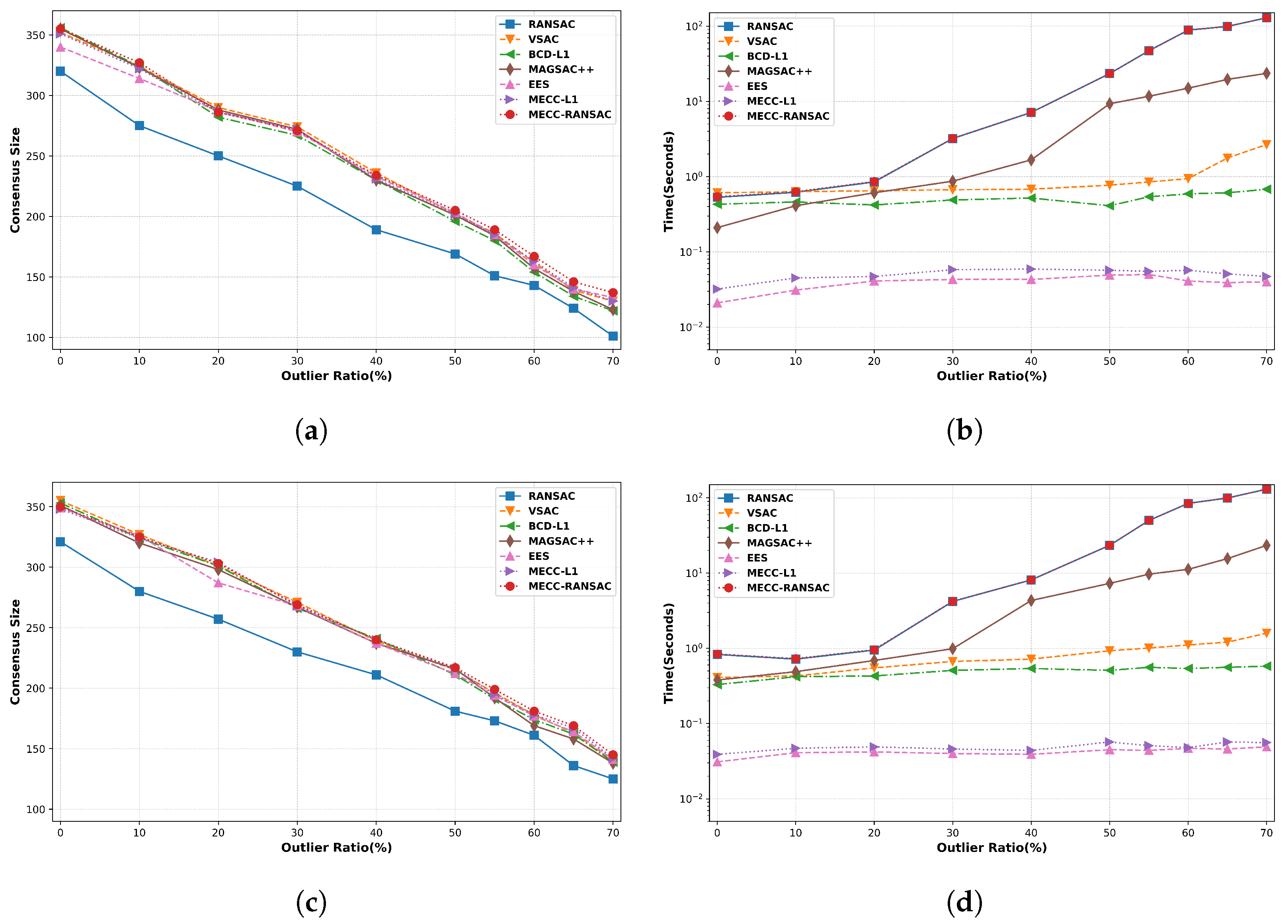
• RANSAC [15]: This iteratively samples a minimal subset of data points to fit a suboptimal model. [Recommended configuration: $\rho =0.99$].
• BCD-L1 [45]: This learns the optimal of the maximum consensus model using the proximal block co-ordinate descent method with initialization using the ${\mathsf{\ell }}_1$ norm method. [Recommended configuration: ${\beta }^{\left(0\right)}=1$, $\gamma =1.01,\delta =1$].
• EES [30]: This utilizes the deterministic annealing method using the linear assignment problem to ensure both efficiency and accuracy. [Recommended configuration: ${\alpha }^{\left(0\right)}=100$, $\gamma =0.9$, $\delta =1$].
• MAGSAC++ [19]: This is a novel class of M-estimators, which is a robust kernel solved by an iteratively reweighted least squares procedure. It is also combined with progressive NAPSAC, a RANSAC-like robust estimator, to improve its performance. [Recommended configuration: $\rho =0.99$];
• VSAC [40]: This is the latest RANSAC-type algorithm, incorporating the concept of independent inliers to enhance its effectiveness in handling dominant planes. It enables the accurate rejection of incorrect models without false positives. [Recommended configuration: $\rho =0.99$].

In our experiments, we adopted a similar initialization strategy to that proposed by [30], which involves minimizing the ${\mathsf{\ell }}_1$ norm using the singular value decomposition (SVD) method. Additionally, we set the hyperparameters as ${\mu }^{\left(k\right)}=0.001$, ${\gamma }^{\left(k\right)}=k/(k+5)$, $\alpha =0.8$, ${\beta }_1=1.11,\mathrm{and}{\beta }_2=1.04$.

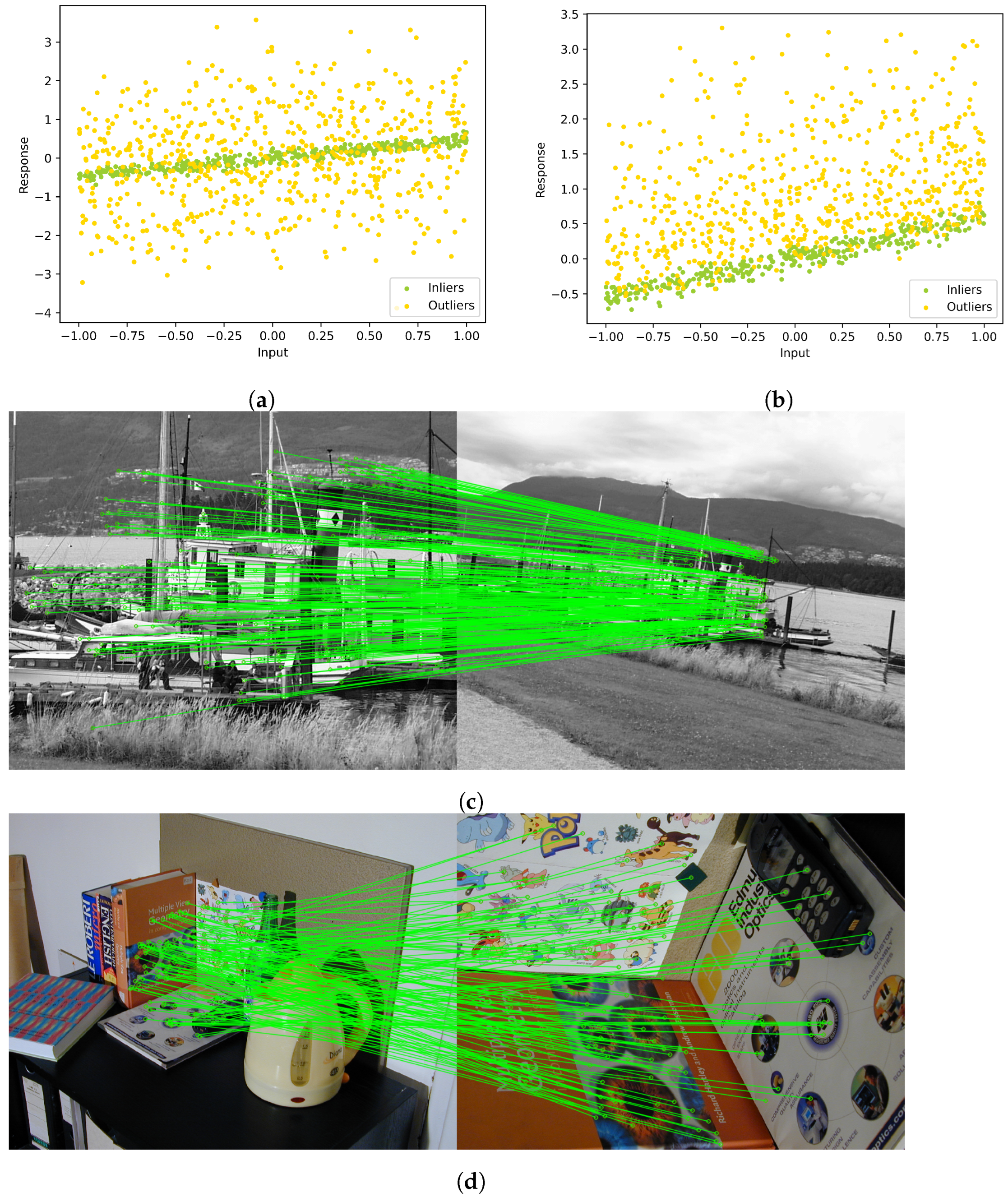
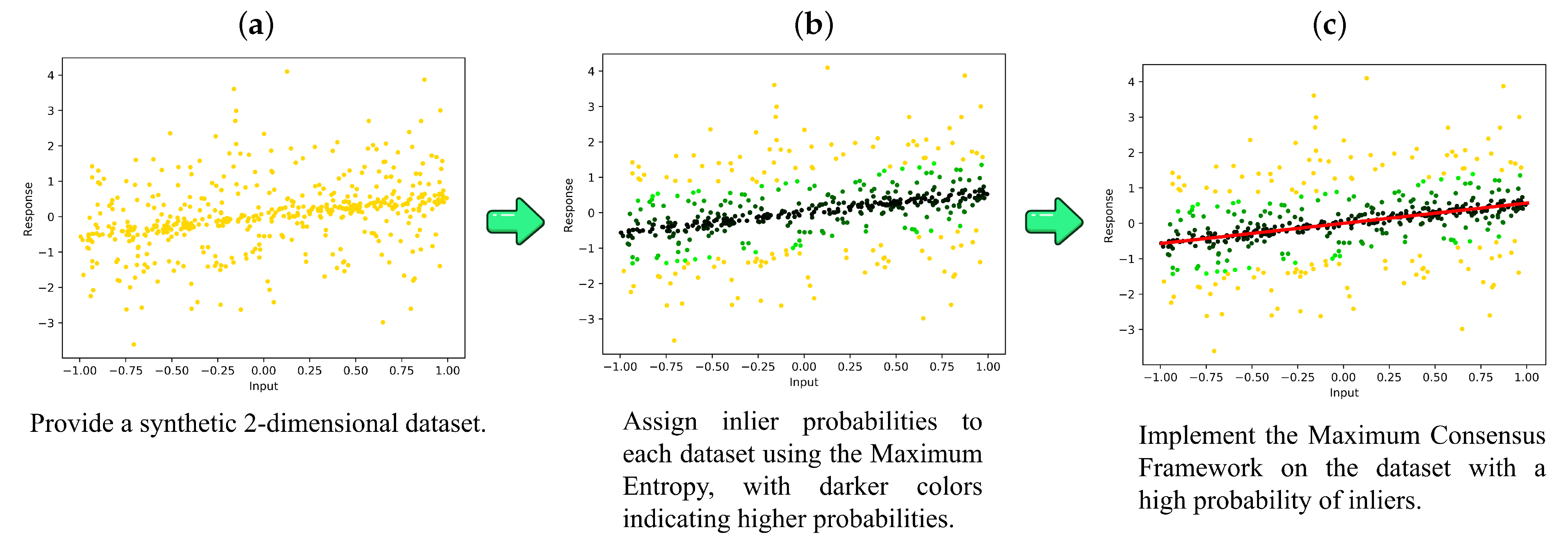
4.1. Robust Linear Regression

Firstly, a synthetic experiment was conducted, which followed the settings of [45]. Specifically, we generated $L=500$ data points from a linear model, $\mathbf{y}=\mathbf{A}\mathit{\theta }$, where $\mathbf{A}\in {\mathbb{R}}^{500\times 8}$ and each element of the matrix follows a random uniform distribution in the range of $\left[-1,1\right]$. Moreover, we contaminated each element of the vector, $\mathbf{y}$, by using white Gaussian noise with a standard deviation of 0.1. In order to simulate outliers, we added additional noise to a randomly selected subset of elements in $\mathbf{y}$ with a much higher level of noise. Our paper considers two different assumptions for generating outliers:

(1)

Balanced data: The outliers in $\mathbf{y}$ were contaminated by using Gaussian noise with a standard deviation of $\sigma =1.2$.

(2)

Unbalanced data: The Gaussian noise was restricted to be positive.

In the case of balanced data, the simulated outliers were distributed evenly on two sides of the hyperplane, whereas for unbalanced data, the simulated outliers were only present on one side. In Figure 1a,b, the distributions of both balanced and unbalanced data are visually presented. Figure 2 provides an overview of our proposed method. Additionally, Figure 3 depicts the average consensus size at termination and runtime (on a logarithmic scale) for the methods evaluated in this study. The average consensus size was obtained by conducting each algorithm on 10 different randomly generated synthetic datasets and then averaging the results. Additionally, we set the threshold as $\delta =0.1$ to identify inliers, which is also considered the inlier-outlier threshold for each method.

In the experimental findings, MECC-RANSAC demonstrates competitive consensus performance, particularly within outlier proportions ranging between $50\%$ and $70\%$. It achieves a comparable performance across various outlier ratios. Conversely, MECC-L1 attains similar performance levels when compared to VSAC, showcasing superiority over other existing methods. Regarding computational efficiency, RANSAC-based methods exhibit an exponential decrease in efficiency as the proportion of outliers increases. In contrast, approaches relying on maximum consensus demonstrate more consistent and efficient performance. However, MECC-RANSAC displays a time-consuming performance pattern similar to that of RANSAC-based methods due to its initialization process. Furthermore, although MECC-L1 does not notably enhance efficiency compared to EES, it demonstrates preferable robustness with negligible performance loss at the millisecond level. This outcome can be attributed to the insufficient credibility of the inliers when the number of outliers exceeds that of the inliers. Our method endeavors to bolster the credibility of inliers by assigning a probability of being an inlier to each data point, thereby exhibiting more pronounced superiority over existing methods, particularly in scenarios with higher outlier proportions. Additionally, utilizing RANSAC for initialization can yield more precise local optima compared to the SVD approach, albeit with some compromise on efficiency.

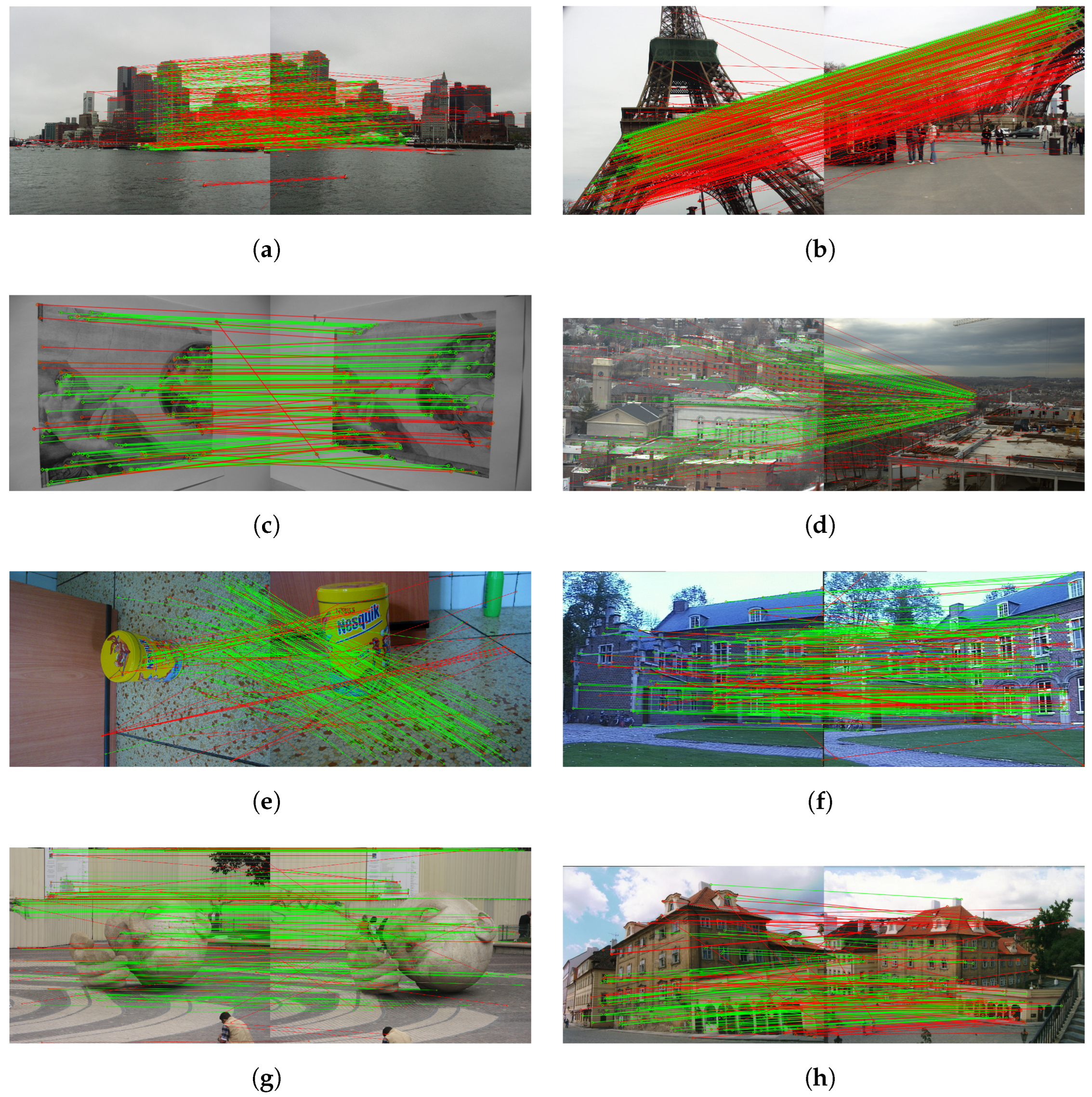
4.2. Fundamental Matrix and Homography Estimation

For the experiments, we established tentative correspondences using the SIFT algorithm [53], with a ratio test of 0.8. The resulting embedding matrix from the fundamental matrix and homography transformation discussed in direct linear transformation is then integrated into Algorithm 1. In addition, the inlier threshold was set as $\delta =2$.

According to the evaluation metrics presented in

Table 2. Quantitative evaluation of homography and fundamental estimation. The dataset names, their corresponding number of image pairs and problems, and the evaluation metrics are shown in the first two columns. The other columns show the average geometric error and proportion of failures over 100 runs, where a test is considered a failure if the average geometric error is greater than $1\%$ of the image diagonal. The mean processing time (in milliseconds) and the summary statistics of all datasets are provided. Bold indicates the best result among the seven compared methods.

Method		RANSAC	BCD-L1	MAGSAC++	EES	VSAC	MECC-L1	MECC-RANSAC
homogr	failure ratio (%)	17.86	14.47	11.08	9.34	9.14	9.20	9.15
16 image pairs	geometric error (pixel)	2.02	1.36	1.19	1.06	1.05	1.04	1.03
$\mathbf{H}$	time (milliseconds)	255.3	97.6	101.5	65.3	70.2	69.7	271.2
EVD	failure ratio (%)	23.27	15.33	17.62	16.37	14.91	14.88	14.69
15 image pairs	geometric error (pixel)	1.80	1.20	1.03	0.97	0.91	0.96	0.93
$\mathbf{H}$	time (milliseconds)	339.1	103.6	143.3	49.3	53.1	51.4	350.9
Hpatches	failure ratio (%)	26.86	10.49	8.61	7.33	6.91	6.74	6.82
142 image pairs	geometric error (pixel)	3.46	1.55	1.34	1.24	1.26	1.23	1.20
$\mathbf{H}$	time (milliseconds)	361.3	94.6	112.5	46.0	74.6	46.3	372.1
kusvod2	failure ratio (%)	21.49	12.01	11.15	9.63	9.20	9.23	9.26
16 image pairs	geometric error (pixel)	2.13	1.41	1.27	0.89	0.90	0.91	0.86
$\mathbf{F}$	time (milliseconds)	348.2	65.4	171.6	34.2	48.2	35.3	362.1
Adelaide	failure ratio (%)	15.23	9.21	7.61	6.99	6.47	6.73	6.54
19 image pairs	geometric error (pixel)	1.48	0.95	0.87	0.78	0.56	0.57	0.53
$\mathbf{F}$	time (milliseconds)	307.4	58.6	143.1	33.7	43.7	34.6	320.1
PhotoTour	failure ratio (%)	20.05	13.32	9.24	7.09	7.18	7.08	7.10
500 image pairs	geometric error (pixel)	1.57	1.05	0.85	0.68	0.61	0.65	0.64
$\mathbf{F}$	time (milliseconds)	292.4	95.9	189.9	40.3	78.1	40.9	333.6
ALL	failure ratio (%)	20.79	12.47	10.89	9.46	8.97	8.98	8.93
	geometric error (pixel)	2.08	1.25	1.09	0.94	0.88	0.89	0.86
708 image pairs	time (milliseconds)	317.28	85.95	143.65	44.80	61.32	46.37	335.00

, we used the average geometric error in both fundamental matrices and homographies, which is calculated as the Sampson distance from the ground truth inliers. Additionally, we reported the proportion of failures in each dataset, where an image pair is considered a failure if the estimated model induces an average geometric error larger than $1\%$ of the image diagonal. Additionally, we employed the consensus size regarding correspondences to assess the qualitative performance, as outlined in both

Table 3. Quantitative evaluation of homography estimation regarding consensus size on 25 image pairs.

Image (Correspondence Size)	RANSAC	BCD-L1	MAGSAC++	EES	VSAC	MECC-L1	MECC-RANSAC
Christ (515)	287	292	295	296	300	297	298
University (603)	471	506	505	508	509	508	510
Bodleian (249)	166	166	168	170	173	173	174
Magdalen (1429)	1286	1285	1288	1289	1291	1288	1290
Radcliffe (287)	169	172	173	175	175	176	177
Aerial I (545)	315	317	318	320	323	320	322
Corridor (490)	374	376	377	377	380	378	379
Kapel (537)	320	322	323	322	325	324	323
Merton II (1125)	845	853	854	855	856	855	856
Merton III (891)	550	548	549	550	551	552	551
Valbonne (505)	269	276	277	278	280	276	278
Boat (1002)	782	779	784	785	788	786	788
Bark (1011)	880	882	885	887	886	884	885
Bikes (2061)	1531	1528	1533	1533	1536	1534	1537
Graff (1444)	800	805	806	805	807	805	806
Trees (1848)	1131	1129	1134	1134	1136	1133	1136
Build 4 (454)	217	204	219	220	224	221	225
Build 5 (873)	550	552	553	557	556	555	554
Build 22 (807)	469	471	473	474	473	471	473
Build 24 (501)	255	258	260	261	264	265	266
Build 28 (504)	232	237	239	241	246	245	248
Build 37 (413)	181	183	184	185	187	185	186
Build 59 (644)	319	324	325	325	326	324	325
Build 67 (571)	231	234	236	235	239	237	240
Build 199 (613)	286	286	288	289	289	290	290

and

Table 4. Quantitative evaluation of fundamental matrix estimation regarding consensus size on 19 image pairs.

Image (Correspondence Size)	RANSAC	BCD-L1	MAGSAC++	EES	VSAC	MECC-L1	MECC-RANSAC
House (656)	240	267	276	277	278	278	280
Aerial (583)	264	285	290	289	290	288	291
Merton (590)	295	317	322	324	326	323	325
Wadham (618)	305	325	333	334	335	334	336
Corridor (684)	310	386	390	390	393	389	391
University Library (439)	224	249	248	251	253	251	254
Christ Church (524)	258	313	315	317	319	319	320
Kapel (449)	160	211	213	215	217	217	217
Invalides (558)	180	228	230	232	232	233	234
Union House (520)	230	288	291	292	291	292	291
Old Classic Wing (561)	310	386	390	390	393	389	391
Ball Hall (538)	170	212	215	217	219	220	220
Build 04 (394)	181	192	197	198	197	196	196
Build 10 (546)	214	252	255	257	259	258	260
Build 23 (699)	315	330	332	332	335	333	334
Build 36 (651)	275	321	322	323	324	322	325
Build 64 (529)	187	235	237	238	240	239	240
Build 81 (525)	262	311	316	317	320	318	320

for homography using 25 image pairs and fundamental matrix estimation using 19 image pairs, respectively. In order to ensure a comprehensive evaluation, we augmented our experimental evaluation by introducing a controlled number of outliers. This augmentation involves the random pairing of two points from the two images, thus generating correspondence data characterized by a predetermined outlier rate for each dataset. We systematically regulated the outlier rate within the range of $30\%$ to $70\%$.

As per the overall evaluation stated in Table 2, Table 3 and Table 4, RANSAC, a classical algorithm, notably suffers from considerable sensitivity towards high outlier proportions in real images. This sensitivity leads to a substantial increase in the time required for geometric estimation. While MAGSAC++ demonstrates heightened stability compared to RANSAC and BCD-L1 across most real image scenarios, it encounters challenges in striking a balance between accuracy and computational efficiency, particularly when dealing with datasets containing numerous outliers.

In the context of the average geometric error, failure rate metrics, and consensus size across all images, MECC-RANSAC displays superior accuracy and robustness compared to other representative algorithms and MECC-L1. However, MECC-RANSAC exhibits limitations in efficiency due to its initialization approach. On the other hand, MECC-L1 incurs a marginally higher time cost compared to EES (approximately 1.57 milliseconds on average). Nevertheless, it showcases improved performance concerning geometric accuracy and failure ratio, which is comparable to VSAC. Furthermore, Figure 4 presents the visual results obtained from our proposed method for both homography estimation and fundamental matrix estimation.

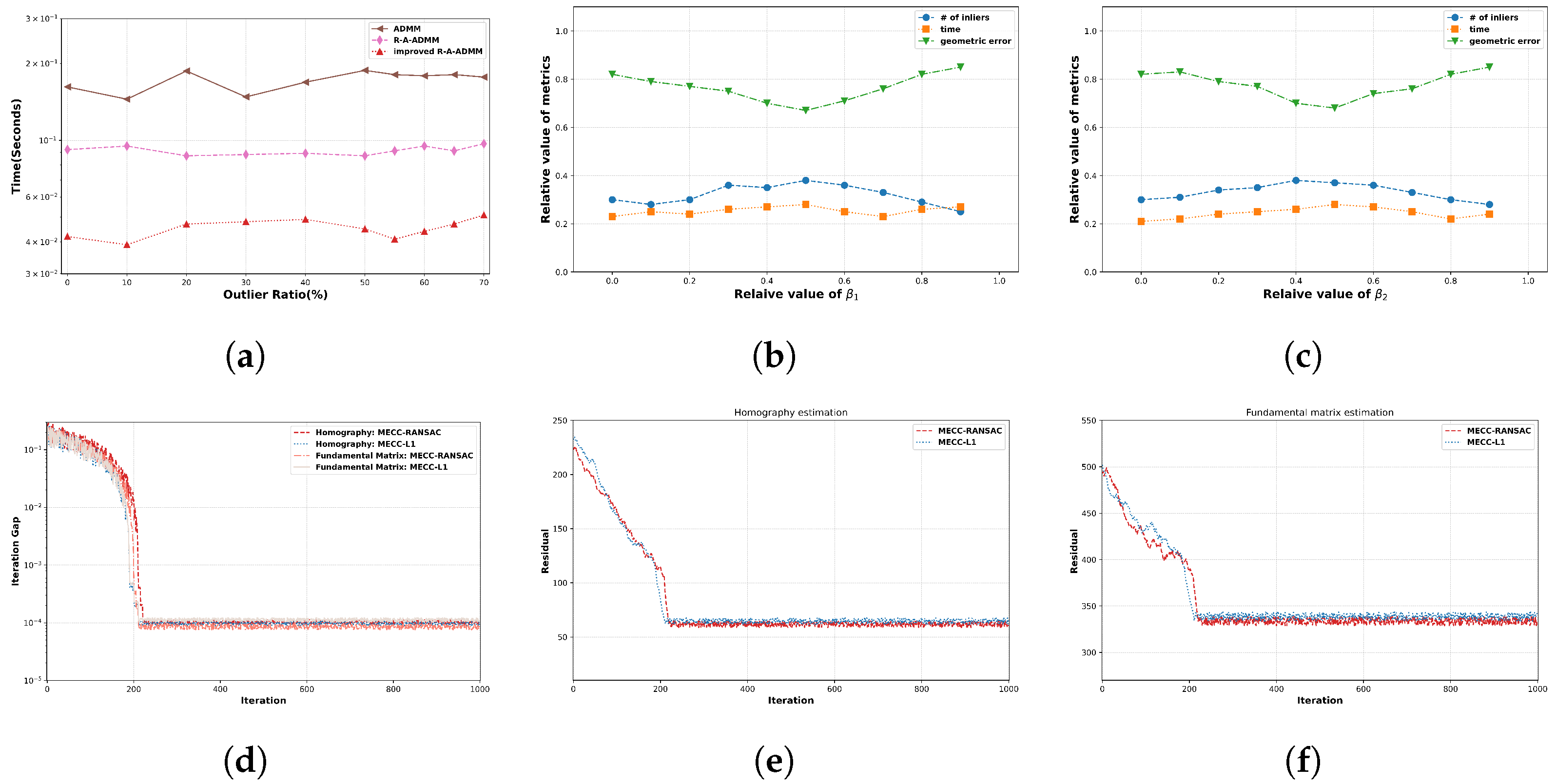
4.3. Algorithmic Analysis

Additional experiments were conducted to elucidate the efficiency discrepancies among ADMM, R-A-ADMM, and the improved R-A-ADMM proposed in this paper for geometry estimation. The outcome presented in Figure 4a demonstrates the efficacy of our introduced enhancements. This improvement stems from the pivotal role of the variable $\mathit{\theta }$’s updating process, which substantively influences the overall time complexity. This inefficiency can be effectively mitigated through the application of the maximization-minimization technique.

In the context of hyperparameter ablation, the consideration was devoted to the selection of scheduling parameters ${\beta }_1$ and ${\beta }_2$, a process guided by an exhaustive array of ablation studies that incorporated execution time, geometric error, and consensus size. The empirical results, showcased in Figure 5b,c, substantiate the robustness of our proposed methodology with regard to the selection of scheduling parameters, affirming its proficiency in maintaining both computational efficiency and accuracy. Figure 5c presents the typical convergence pattern of the improved ADMM algorithm initialized using RANSAC and the minimizing ${\mathsf{\ell }}_1$ norm. This assessment was conducted through the evaluation of the iteration gap of the variable $\mathit{\theta }$, defined as $1/\sqrt{D}{∥{\mathit{\theta }}^{(k+1)}-{\mathit{\theta }}^k∥}_2$ using HPatches for homography and PhotoTour for fundamental matrix estimation. Furthermore, Figure 5d,e depict another common convergence behavior of the improved ADMM algorithm with RANSAC and ${\mathsf{\ell }}_1$ norm-based initialization, evaluated by using the ${\mathsf{\ell }}_2$ norm of the residual $|\mathbf{X}\mathit{\theta }-\mathbf{y}|$. These visualizations collectively demonstrate that the MECC methodology can further explore more locally optimal solutions subsequent to the initialization process based on RANSAC and the minimizing ${\mathsf{\ell }}_1$ norm process. Moreover, this approach mitigates trivial solution issues, as the ADMM-based optimizer specifically explores better solutions within the vicinity of the local optima obtained from RANSAC and least square fitting.

5. Conclusions

This study proposes a novel maximum consensus strategy that leverages the maximum entropy framework to estimate the probability distribution of inliers. The proposed novel maximum consensus strategy is solved using an improved version of R-A-ADMM. The proposed method is capable of distinguishing inliers and outliers in contaminated datasets and efficiently handling datasets with a high proportion of outliers. Our experimental evaluations validate the performance of the proposed method, particularly when initialized using RANSAC, exhibiting heightened geometric accuracy and a reduced failure ratio compared to existing state-of-the-art algorithms. This enhanced performance is notably observed in scenarios where there is a significant presence of outliers across synthetic and real datasets utilized for fundamental matrix and homography estimation. However, it is essential to acknowledge that the efficiency of this approach is constrained due to its reliance on the specific initialization methodology. Conversely, our method employing the least squares fitting approach shows slightly diminished accuracy and robustness compared to RANSAC initialization. Nevertheless, it maintains competitiveness across accuracy, robustness, and efficiency metrics when benchmarked against other existing algorithms. The marginal increase in computational expense, approximately at the millisecond level compared to EES, does not notably affect the overall performance. The limitation of the proposed method arises from its dependence on the chosen initialization for achieving locally optimal solutions and circumventing trivial solution issues in direct linear transformation. As a result, our future study will concentrate on minimizing the influence of initialization within our framework. Overall, the proposed method provides promising efficiency in addressing the intricate challenges of geometric estimation in the presence of outliers.

References

1. Isack, H.; Boykov, Y. Energy-based geometric multi-model fitting. Int. J. Comput. Vis. 2012, 97, 123–147. [Google Scholar] [CrossRef]
2. Pham, T.T.; Chin, T.-J.; Schindler, K.; Suter, D. Interacting geometric priors for robust multimodel fitting. IEEE Trans. Image Process. 2014, 23, 4601–4610. [Google Scholar] [CrossRef] [PubMed]
3. Brown, M.; Lowe, D.G. Automatic panoramic image stitching using invariant features. Int. J. Comput. Vis. 2007, 74, 59–73. [Google Scholar] [CrossRef]
4. Pritchett, P.; Zisserman, A. Wide baseline stereo matching. In Proceedings of the Sixth International Conference on Computer Vision (IEEE Cat. No. 98CH36271), Bombay, India, 7 January 1998; pp. 754–760. [Google Scholar]
5. Matas, J.; Chum, O.; Urban, M.; Pajdla, T. Robust wide-baseline stereo from maximally stable extremal regions. Image Vis. Comput. 2004, 22, 761–767. [Google Scholar] [CrossRef]
6. Mishkin, D.; Matas, J.; Perdoch, M. Mods: Fast and robust method for two-view matching. Comput. Vis. Image Underst. 2015, 141, 81–93. [Google Scholar] [CrossRef]
7. Meer, P. Robust techniques for computer vision. Emerg. Top. Comput. Vis. 2004, 2004, 107–190. [Google Scholar]
8. Martinec, D.; Pajdla, T. Robust rotation and translation estimation in multiview reconstruction. In Proceedings of the 2007 IEEE Conference on Computer Vision and Pattern Recognition, Minneapolis, MN, USA, 17–22 June 2007; pp. 1–8. [Google Scholar]
9. Mur-Artal, R.; Montiel, J.M.M.; Tardos, J.D. Orb-slam: A versatile and accurate monocular slam system. IEEE Trans. Robot. 2015, 31, 1147–1163. [Google Scholar] [CrossRef]
10. Abdigapporov, S.; Miraliev, S.; Kakani, V.; Kim, H. Joint multiclass object detection and semantic segmentation for autonomous driving. IEEE Access 2023, 11, 37637–37649. [Google Scholar] [CrossRef]
11. Abdigapporov, S.; Miraliev, S.; Alikhanov, J.; Kakani, V.; Kim, H. Performance comparison of backbone networks for multi-tasking in self-driving operations. In Proceedings of the 2022 22nd International Conference on Control, Automation and Systems (ICCAS), Jeju, Republic of Korea, 27 November–1 December 2022; pp. 819–824. [Google Scholar]
12. Irfan, M.; Munsif, M.V. Deepdive: A learning-based approach for virtual camera in immersive contents. Virtual Real. Intell. Hardw. 2022, 4, 247–262. [Google Scholar] [CrossRef]
13. Ullah, M.; Amin, S.U.; Munsif, M.; Yamin, M.M.; Safaev, U.; Khan, H.; Khan, S.; Ullah, H. Serious games in science education: A systematic literature. Virtual Real. Intell. Hardw. 2022, 4, 189–209. [Google Scholar] [CrossRef]
14. Chum, O.; Matas, J.; Kittler, J. Locally optimized ransac. In Proceedings of the Pattern Recognition: 25th DAGM Symposium, Magdeburg, Germany, 10–12 September 2003; Springer: Berlin/Heidelberg, Germany, 2003; pp. 236–243. [Google Scholar]
15. Fischler, M.A.; Bolles, R.C. Random sample consensus: A paradigm for model fitting with applications to image analysis and automated cartography. Commun. ACM 1981, 24, 381–395. [Google Scholar] [CrossRef]
16. Lebeda, K.; Matas, J.; Chum, O. Fixing the locally optimized ransac–full experimental evaluation. In Proceedings of the British Machine Vision Conference, Citeseer Princeton, NJ, USA, 3–7 September 2012. [Google Scholar]
17. Jo, G.; Lee, K.-S.; Chandra, D.; Jang, C.-H.; Ga, M.-H. Ransac versus cs-ransac. In Proceedings of the AAAI Conference on Artificial Intelligence, Austin, TX, USA, 25–30 January 2015; Volume 29. [Google Scholar]
18. Wei, T.; Patel, Y.; Shekhovtsov, A.; Matas, J.; Barath, D. Generalized differentiable ransac. In Proceedings of the IEEE/CVF International Conference on Computer Vision, Paris, France, 4–6 October 2023; pp. 17649–17660. [Google Scholar]
19. Barath, D.; Noskova, J.; Ivashechkin, M.; Matas, J. Magsac++, a fast, reliable and accurate robust estimator. In Proceedings of the IEEE/CVF Conference on Computer Vision and Pattern Recognition, Seattle, WA, USA, 13–19 June 2020; pp. 1304–1312. [Google Scholar]
20. Barath, D.; Matas, J. Graph-cut ransac: Local optimization on spatially coherent structures. IEEE Trans. Pattern Anal. Mach. Intell. 2021, 44, 4961–4974. [Google Scholar] [CrossRef] [PubMed]
21. Chum, O.; Matas, J. Matching with prosac-progressive sample consensus. In Proceedings of the 2005 IEEE Computer Society Conference on Computer Vision and Pattern Recognition (CVPR’05), Diego, CA, USA, 20–25 June 2005; pp. 220–226. [Google Scholar]
22. Olsson, C.; Enqvist, O.; Kahl, F. A polynomial-time bound for matching and registration with outliers. In Proceedings of the 2008 IEEE Conference on Computer Vision and Pattern Recognition, Anchorage, AK, USA, 23–28 June 2008; pp. 1–8. [Google Scholar]
23. Zheng, Y.; Sugimoto, S.; Okutomi, M. Deterministically maximizing feasible subsystem for robust model fitting with unit norm constraint. In Proceedings of the CVPR 2011, Colorado Springs, CO, USA, 20–25 June 2011; pp. 1825–1832. [Google Scholar]
24. Enqvist, O.; Ask, E.; Kahl, F.; Åström, K. Robust fitting for multiple view geometry. In Proceedings of the Computer Vision–ECCV 2012: 12th European Conference on Computer Vision, Florence, Italy, 7–13 October 2012; Springer: Berlin/Heidelberg, Germany, 2012; pp. 738–751. [Google Scholar]
25. Li, H. Consensus set maximization with guaranteed global optimality for robust geometry estimation. In Proceedings of the 2009 IEEE 12th International Conference on Computer Vision, Kyoto, Japan, 29 September–2 October 2009; pp. 1074–1080. [Google Scholar]
26. Cai, Z.; Chin, T.-J.; Le, H.; Suter, D. Deterministic consensus maximization with biconvex programming. In Proceedings of the European Conference on Computer Vision (ECCV), Mulish, Germany, 8–14 September 2018; pp. 685–700. [Google Scholar]
27. Le, H.; Chin, T.-J.; Eriksson, A.; Do, T.-T.; Suter, D. Deterministic approximate methods for maximum consensus robust fitting. IEEE Trans. Pattern Anal. Mach. Intell. 2019, 43, 842–857. [Google Scholar] [CrossRef] [PubMed]
28. Park, D.H.; Kakani, V.; Kim, H. Automatic radial un-distortion using conditional generative adversarial network. J. Inst. Control. Robot. Syst. 2019, 25, 1007–1013. [Google Scholar] [CrossRef]
29. Kakani, V.; Kim, H. Adaptive self-calibration of fisheye and wide-angle cameras. In Proceedings of the TENCON 2019-2019 IEEE Region 10 Conference (TENCON), Kochi, India, 17–20 October 2019; pp. 976–981. [Google Scholar]
30. Fan, A.; Ma, J.; Jiang, X.; Ling, H. Efficient deterministic search with robust loss functions for geometric model fitting. IEEE Trans. Pattern Anal. Mach. Intell. 2021, 44, 8212–8229. [Google Scholar] [CrossRef]
31. Ghimire, A.; Kakani, V.; Kim, H. Ssrt: A sequential skeleton rgb transformer to recognize fine-grained human-object interactions and action recognition. IEEE Access 2023, 11, 51930–51948. [Google Scholar] [CrossRef]
32. França, G.; Robinson, D.P.; Vidal, R. A nonsmooth dynamical systems perspective on accelerated extensions of admm. IEEE Trans. Autom. Control. 2023, 68, 2966–2978. [Google Scholar] [CrossRef]
33. Torr, P.H.; Nasuto, S.J.; Bishop, J.M. Napsac: High noise, high dimensional robust estimation-it’s in the bag. Br. Mach. Vis. Conf. (BMVC) 2002, 2, 3. [Google Scholar]
34. Ni, K.; Jin, H.; Dellaert, F. Groupsac: Efficient consensus in the presence of groupings. In Proceedings of the 2009 IEEE 12th International Conference on Computer Vision, Kyoto, Japan, 29 September–2 October 2009; pp. 2193–2200. [Google Scholar]
35. Fragoso, V.; Sen, P.; Rodriguez, S.; Turk, M. Evsac: Accelerating hypotheses generation by modeling matching scores with extreme value theory. In Proceedings of the IEEE International Conference on Computer Vision, Sydney, Australia, 1–8 December 2013; pp. 2472–2479. [Google Scholar]
36. Torr, P.H.; Zisserman, A. Mlesac: A new robust estimator with application to estimating image geometry. Comput. Vis. Image Underst. 2000, 78, 138–156. [Google Scholar] [CrossRef]
37. Torr, P.H.S. Bayesian model estimation and selection for epipolar geometry and generic manifold fitting. Int. J. Comput. Vis. 2002, 50, 35–61. [Google Scholar] [CrossRef]
38. Barath, D.; Matas, J. Graph-cut ransac. In Proceedings of the IEEE Conference on Computer Vision and Pattern Recognition, Salt Lake City, UT, USA, 18–23 June 2018; pp. 6733–6741. [Google Scholar]
39. Barath, D.; Matas, J.; Noskova, J. Magsac: Marginalizing sample consensus. In Proceedings of the IEEE/CVF Conference on Computer Vision and Pattern Recognition, Long Beach, CA, USA, 15–20 June 2019; pp. 10197–10205. [Google Scholar]
40. Ivashechkin, M.; Barath, D.; Matas, J. Vsac: Efficient and accurate estimator for h and f. In Proceedings of the IEEE/CVF International Conference on Computer Vision, Montreal, BC, Canada, 11–17 October 2021; pp. 15243–15252. [Google Scholar]
41. Bazin, J.-C.; Li, H.; Kweon, I.S.; Demonceaux, C.; Vasseur, P.; Ikeuchi, K. A branch-and-bound approach to correspondence and grouping problems. IEEE Trans. Pattern Anal. Mach. Intell. 2012, 35, 1565–1576. [Google Scholar] [CrossRef] [PubMed]
42. Chin, T.-J.; Purkait, P.; Eriksson, A.; Suter, D. Efficient globally optimal consensus maximisation with tree search. In Proceedings of the IEEE Conference on Computer Vision and Pattern Recognition, Boston, MA, USA, 7–12 June 2015; pp. 2413–2421. [Google Scholar]
43. Cai, Z.; Chin, T.-J.; Koltun, V. Consensus maximization tree search revisited. In Proceedings of the IEEE/CVF International Conference on Computer Vision, Seoul, Republic of Korea, 27 October–2 November 2019; pp. 1637–1645. [Google Scholar]
44. Chin, T.-J.; Kee, Y.H.; Eriksson, A.; Neumann, F. Guaranteed outlier removal with mixed integer linear programs. In Proceedings of the IEEE Conference on Computer Vision and Pattern Recognition, Las Vegas, NV, USA, 26 June –1 July 2016; pp. 5858–5866. [Google Scholar]
45. Wen, F.; Ying, R.; Gong, Z.; Liu, P. Efficient algorithms for maximum consensus robust fitting. IEEE Trans. Robot. 2019, 36, 92–106. [Google Scholar] [CrossRef]
46. Ke, Q.; Kanade, T. Quasiconvex optimization for robust geometric reconstruction. IEEE Trans. Pattern Anal. Mach. Intell. 2007, 29, 1834–1847. [Google Scholar] [CrossRef]
47. Olsson, C.; Eriksson, A.; Hartley, R. Outlier removal using duality. In Proceedings of the 2010 IEEE Computer Society Conference on Computer Vision and Pattern Recognition, San Francisco, CA, USA, 13–18 June 2010; pp. 1450–1457. [Google Scholar]
48. Boyd, S.; Parikh, N.; Chu, E.; Peleato, B.; Eckstein, J. Distributed optimization and statistical learning via the alternating direction method of multipliers. Found. Trends® Mach. Learn. 2011, 3, 1–122. [Google Scholar]
49. Goldstein, T.; O’Donoghue, B.; Setzer, S.; Baraniuk, R. Fast alternating direction optimization methods. SIAM J. Imaging Sci. 2014, 7, 1588–1623. [Google Scholar] [CrossRef]
50. Yang, J.; Zhang, Y. Alternating direction algorithms for ∖ell_1-problems in compressive sensing. SIAM J. Sci. Comput. 2011, 33, 250–278. [Google Scholar] [CrossRef]
51. Balntas, V.; Lenc, K.; Vedaldi, A.; Mikolajczyk, K. Hpatches: A benchmark and evaluation of handcrafted and learned local descriptors. In Proceedings of the IEEE Conference on Computer Vision and Pattern Recognition, Honolulu, HI, USA, 21–26 July 2017; pp. 5173–5182. [Google Scholar]
52. Snavely, N.; Seitz, S.M.; Szeliski, R. Photo tourism: Exploring photo collections in 3d. In Proceedings of the ACM Siggraph 2006 Papers, Boston, MA, USA, 30 July–3 August 2006; pp. 835–846. [Google Scholar]
53. Lowe, D.G. Distinctive image features from scale-invariant keypoints. Int. J. Comput. Vis. 2004, 60, 91–110. [Google Scholar] [CrossRef]
Figure 1. Two-dimensional analogy of (a) balanced (b) unbalanced data generated in our experiments. Representative examples of our proposed method for (c) homography matrix and (d) fundamental matrix estimation, where the green lines represent detected inlier correspondences.
Electronics 13 02972 g001
Figure 2. Overview of maximum entropy with consensus constraints (MECC). In (a), a two-dimensional representation of balanced data with a 60 % outlier ratio is provided. In (b), each point is categorized as either an inlier or an outlier. (c) Green represents the detected inliers, while red represents the outliers. Each data point is assigned an inlier probability, with darker colors indicating higher probabilities. This demonstrates that by focusing on data points with higher inlier probabilities, our methodology can robustly estimate potential geometric relationships in datasets with a high outlier ratio, as depicted by the red line.
Electronics 13 02972 g002
Figure 3. Average qualitative results for robust linear regression with 10 different randomly generated synthetic datasets ( L = 500 and D = 8 ). (a) Consensus size with balanced data. (b) Runtime with balanced data. (c) Consensus size with unbalanced data. (d) Runtime with unbalanced data.
Electronics 13 02972 g003
Figure 4. Visual results obtained from our proposed method are demonstrated for (ad) homography estimation from homogr and (eh) fundamental matrix estimation from kusvod2. In the visuals, the green and red lines correspond to detected inlier and outlier correspondences, respectively.
Electronics 13 02972 g004
Figure 5. (a) A comparative assessment of the efficiency of the ADMM-based solution using synthetic data. (b,c) Graphical representations depicting the variation in the number of inliers, processing time, and geometric error as a function of the scheduling parameters β 1 and β 2 , employing HPatches. (d) Illustration showcasing the typical convergence behavior of the improved ADMM algorithm, initialized using RANSAC and 1 norm, observing the iteration gap of θ using HPatches for homography and PhotoTour for fundamental matrix estimation. Typical convergence behavior of the improved ADMM with RANSAC and 1 norm-based initialization, focusing on the residual metric and using (eHPatches for homography and (f) PhotoTour for fundamental matrix estimation.
Electronics 13 02972 g005