Supraharmonics Reconstruction Method Based on Blackman Window and Compressed Sensing

Abstract

This paper proposes a method that combines window functions with compressed sensing for the detection of ultra-high harmonics in the frequency range of 2–150 kHz. By analyzing the sparsity of the signal, the Bruckmann window function, which is most suitable for the compressed sensing reconstruction process and the characteristics of ultra-high harmonics, is selected. Simulations indicate that, compared to existing methods, the proposed algorithm based on the fusion of the Bruckmann window and compressed sensing achieves a sparser post-observation signal with reduced fluctuations. The robustness and anti-interference capabilities are enhanced, while the harmonic detection accuracy and signal reconstruction performance are significantly improved. The reconstruction error reaches 4.15 × 10⁻⁶, the mean squared error percentage (MSE) reaches 4.13 × 10⁻⁶, and the signal-to-noise ratio (SNR) is as high as 97.69 dB, marking an increase of 54.11%. This study provides a new theoretical and methodological approach for the analysis and processing of ultra-high harmonics caused by a high proportion of power electronic devices.

1. Introduction

As the proportion of new energy sources integrated into distribution networks continues to increase, the widespread application of multi-level power electronic devices based on Insulate-Gate Bipolar Transistor (IGBT) has become inevitable. The growing prevalence of high switching frequency power electronic converters has resulted in more frequent and complex interactions between devices [1,2], profoundly transforming the power harmonic emission characteristics of distribution networks. These characteristics are evolving from low-order harmonics to ultra-high-order, wide-frequency harmonics [3], with a significant increase from 2 kHz to 150 kHz ultra-high-order harmonics (supraharmonics) distortions [4,5,6]. This phenomenon has emerged as a new power quality issue [7,8], constantly threatening the safe and stable operation of the energy internet [9,10,11,12].

The sources of ultra-high-order harmonics mainly include BJT half-bridge resonators, grid-connected inverters, Power Factor Correction (PFC) circuits, and full-power converters of wind turbines [13,14,15,16,17,18]. Several methods have been proposed to address ultra-high-order harmonics, such as the Infinite Impulse Response (IIR) filter method introduced in 2014 [19,20], the wavelet packet transform method proposed in 2018 [21], analog filters, and the secondary sampling method [22]. While these methods can effectively extract information about ultra-harmonic phenomena, they still exhibit deficiencies in amplitude and frequency band representation. In 2019, a new method for analyzing ultra-high-order harmonics based on compressed sensing (CS) was proposed [23]. This method can overcome the limitations of the FFT algorithm, significantly reduce computation time, and accurately calculate the amplitude and phase of ultra-high-order harmonics. Clearly, the CS algorithm is well-suited for reconstructing ultra-high-order harmonics. However, when CS processing discretizes the ultra-high-order harmonic signal, the originally concentrated energy disperses into broader frequency bands, causing spectral leakage and impacting reconstruction accuracy [24].

To address the issue of significant spectral leakage in the compressed sensing algorithm, this paper applies window functions to signals to reduce fence effects and spectral leakage within the 2 kHz to 150 kHz frequency range. Based on compressed sensing, we propose a method that combines the Blackman window and compressed sensing algorithms for observing and reconstructing ultra-high-order harmonics. By leveraging the advantages of both approaches, we analyze the impact of window functions on signal sparsification and reconstruction accuracy. Instead of focusing on the main and sidelobe analysis of the window function, we select the most suitable Blackman window function based on its effect on the energy distribution of the compressed sensing observation vector. Concurrently, we use compressed sensing technology to reconstruct ultra-high-order harmonics, aiming to reduce spectral leakage and improve signal reconstruction accuracy.

2. Sampling Principle of Compressed Sensing

Compressed sensing (CS) was first proposed by Candes and Donoho, challenging the traditional Nyquist sampling theorem by demonstrating that it is possible to reconstruct a signal perfectly with far fewer samples than conventionally required [25]. This breakthrough has introduced new methodologies for signal processing, image recovery, and compression algorithms. Today, compressed sensing is widely applied in various fields, including network communications, radar measurement, image processing, medical imaging, and biosensing. The technique reduces the number of required samples, decreases data storage needs, enhances data transmission speed, etc.

It is assumed that the dimension of the original signal $x$ is $N\times 1$, and after $x$ has been compressed and sampled by a measurement matrix $\Phi$ of size $M\times N\left(M<<N\right)$, an $M\times 1$ dimensional observation vector $y$ is obtained. Thus, the data amount of observation vector $y$ is much smaller than that of the signal $x$. Figure 1 shows the basic compression process of compressed sensing sampling.

Assuming the original signal $x$ has dimensions $N\times 1$, after being compressed and sampled through a measurement matrix Φ of size $M\times N(M<<N)$, an observation vector $y$ of dimensions $M\times 1$ is obtained. Therefore, the measurement values $y$ obtained are significantly smaller than the data amount of the signal. Figure 1 illustrates the specific compression process of compressed sensing sampling.

Compressed sensing can achieve accurate signal recovery with significantly fewer samples than traditional methods. A critical prerequisite is that the signal must be sparse in some domain. If the signal $x\in R^N$ has $K$ significant non-zero components $({‖x‖}_0\le K)$, then it is $K$-sparse. Furthermore, if these components can be represented in an orthogonal basis, the signal can be expressed as follows:

$$x={\displaystyle \sum _{i=1}^N{\mathit{\theta }}_i{\psi }_i}=\psi \mathit{\theta }$$

(1)

where $\psi \left(\psi ={\left[{\psi }_1,{\psi }_2,\dots {\psi }_N\right]}^T\right)$ represents the orthogonal basis, and $\mathit{\theta }$ denotes the coefficients in this representation.

In most practical applications, the signal $x$ does not fully satisfy the definition of $K$-sparsity. However, when the absolute values of its elements are sorted in descending order, they exhibit a power-law decay characteristic. Such signals are referred to as compressible signals.

When there are only $K$ non-zero items in the sparse coefficient $\mathit{\theta }$, a measurement matrix $\Phi$ of size $M\times N$ is used to process the signal $x$, and an observation vector of size $M\times 1$ is obtained. The process is expressed as follows:

$$y=\mathsf{\Phi }x=\mathsf{\Phi }\Psi \mathit{\theta }$$

(2)

The measurement matrix $\mathsf{\Phi }$ must be chosen as a dense matrix that satisfies the Restricted Isometry Property (RIP) condition.

Theorem 1. 

If there is a constant ${\delta }_k\in (0,1)$ such that Formula (3) holds for all $x\in {\displaystyle {\sum }_k}$, then the matrix $\Phi$ satisfies the K-order RIP condition [26].

$$(1-{\delta }_k){‖x‖}_2^2\le {‖\Phi x‖}_2^2\le (1+{\delta }_k){‖x‖}_2^2$$

(3)

Currently, Gaussian random matrices are commonly used as typical measurement matrices in compressed sensing due to their high reconstruction accuracy attributed to their randomness. Therefore, in this work, we also select Gaussian random matrices as the measurement matrix.

For sparse or compressible signals, the amount of data MMM that need to be collected should satisfy Equation (4).

$$M>c\cdot K\cdot \log (N/K)$$

(4)

where $c$ is a constant, $K$ is the sparsity, and $N$ is the signal length. In practice, the observations $y$ can be regarded as the result of the original signal $x$ undergoing linear projection through the measurement matrix $\Phi$. Using a compressed sensing algorithm, the original signal $x$ can be reconstructed from the measurement matrix $\Phi$ and the observation vector $y$. This process can be viewed as solving or approximately solving a linear convex optimization problem $\mathit{\theta }$, resulting in the estimated value $\widehat{\mathit{\theta }}$. As shown in Equation (5),

$$\begin{array}{l}\widehat{\mathit{\theta }}=\min {‖{\psi }^{T}x‖}_0\end{array}\hspace{1em}s.t.y=\mathsf{\Phi }x=\mathsf{\Phi }\Psi \mathit{\theta }$$

(5)

Since the implementation of the compressed sensing algorithm requires the original signal to be sparse or transformable to a sparse representation, it is necessary to further analyze the impact of using a window function on the sparsity and reconstruction performance of the signal in Section 3.

3. Signal Observation Based on Fusion of Window Functions and Compressed Sensing

3.1. Ultra-High Harmonics Based on Window Function

Compressed sensing of ultra-high-order harmonic signals involves using undersampling methods to analyze the signal over a finite time interval. After discretizing the original signal, spectral distortion occurs, causing the originally concentrated energy to spread into other broader frequency bands, known as spectral leakage, which, in turn, affects the accuracy of signal reconstruction. The principle of the window function is to reduce spectral leakage of the sampled signal by applying a window to the signal, thereby improving measurement accuracy. Suppose the ultra-high-order harmonic is a periodic signal, represented as follows:

$$x(t)={\displaystyle \sum _{i=0}^p{A}_i\cos (2\pi f_i+{\varphi }_i)}$$

(6)

where $f_i$, $A_i$, and ${\varphi }_i$ are the frequency, amplitude, and phase angle of the $i$-th harmonic, and $p$ is the highest number of the considered harmonics. A discretization of the above equation for frequency $f_s$ yields the sequence $x\left(n\right)$:

$$x(n)=x(n{T}_s)={\displaystyle \sum _{i=0}^p{A}_i\cos (n{\omega }_i+{\varphi }_i)}$$

(7)

where $T_s=1/f_s$ is the sampling period, ${\omega }_i=2\pi f_i{T}_s$, and the spectrum of $x\left(n\right)$ is represented by Equation (8):

$$X(e^{j\omega })={\displaystyle \sum _{i=0}^p[}\frac{A_i}{2}{e}^{j{\varphi }_i}\delta (\omega -{\omega }_i)+\frac{A_i}{2}{e}^{-j{\varphi }_i}\delta (\omega +{\omega }_i)]$$

(8)

Let the discrete window function be $w\left(\mathrm{n}\right)$, whose spectrum $W\left({\mathrm{e}}^{\mathrm{j}\omega }\right)$ can be expressed as follows:

$$W(e^{j\omega })=W_0(\omega )\cdot e^{-jc\omega }$$

(9)

where $W_0(\omega )$ is a real function, and $c$ is a constant. A window sequence $w\left(\mathrm{n}\right)$ of length $N$ is used to truncate $x(n)$ in a weighted manner to obtain the signal $x_w(n)$.

$$x_w(n)=x(n)\cdot w(n) n=0,1,2,\cdots N-1$$

(10)

The spectrum of $x_w\left(n\right)$ is represented in Equation (11) [26].

$$\begin{array}{l}{X}_w(e^{j\omega })=X(e^{j\omega })\ast W(e^{j\omega })\\ \hspace{1em}\hspace{1em}\hspace{1em}={\displaystyle \sum _{i=0}^p\left\{\begin{array}{c}\frac{A_i}{2}{W}_0(\omega -{\omega }_i)e^{-j\left[c(\omega -{\omega }_i)-{\varphi }_i\right]}+\\ \frac{A_i}{2}{W}_0(\omega -{\omega }_i)e^{-j\left[c(\omega +{\omega }_i)+{\varphi }_i\right]}\end{array}\right\}}\end{array}$$

(11)

3.2. Signal Sparsity Based on Window Functions and Compressed Sensing

The advantage of windowing is its ability to reduce spectral leakage of the signal, with the key focus being on selecting an appropriate window function. In traditional harmonic analysis, the selection of a window function typically prioritizes a narrow main lobe, low sidelobes, and fast sidelobe amplitude decay, along with considerations of computational load and specific application scenarios. However, currently, ultra-high-order harmonics are best analyzed using compressed sensing methods. When applying window functions in compressed sensing algorithms, it is not sufficient to choose based solely on the traditional criteria of the window function itself. This is because compressed sensing imposes strict requirements on the sampled signal. CS requires the observed signal to be sparse, meaning that when the original signal is projected onto a sparse basis, the absolute values of most of its coefficients are very small. As analyzed above, the observation process in compressed sensing is given by Equation (12). Substituting the windowed signal $x_w(n)=x(n)\cdot w(n)$ into Equation (12), the observation process with the windowed signal is obtained as follows:

$$y_w=\mathsf{\Phi }{x}_w=\mathsf{\Phi }\cdot (x\cdot w)=\mathsf{\Phi }\Psi {\mathit{\theta }}_w$$

(12)

The CS reconfiguration signal then becomes

$${\widehat{x}}_w=\psi \cdot {\mathit{\theta }}_w$$

(13)

It is evident that the use of window functions with different mathematical characteristics modifies the sparse coefficients ${\mathit{\theta }}_w$ corresponding to the sparse basis of the decomposed original signal, thereby influencing the signal reconstruction performance. In the process of applying windows in CS for ultra-high-order harmonics, it is essential to consider the specific characteristics of ultra-high-order harmonic signals and the energy distribution after sparse sampling. This consideration is necessary to select a window function that is suitable for both ultra-high-order harmonics and compressed sensing.

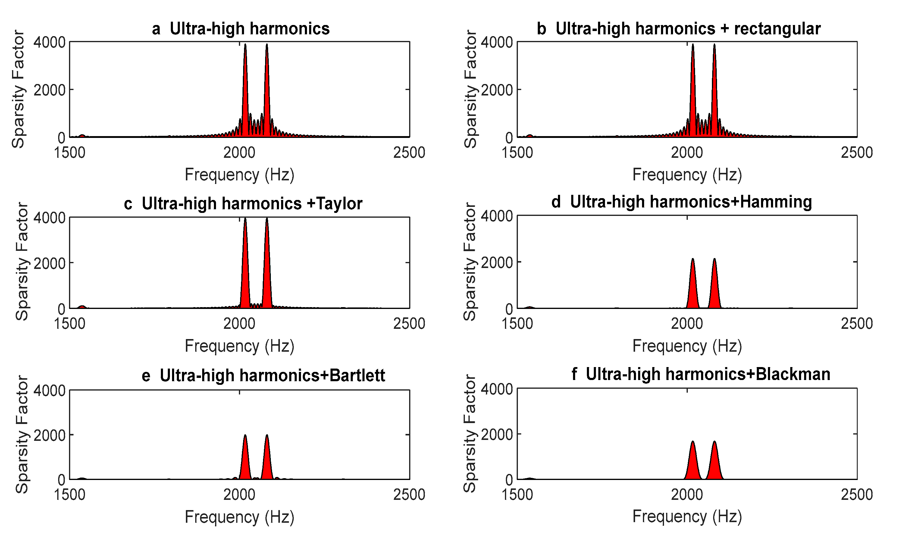
CS theory presupposes that the observed signal satisfies sparsity, a condition that must also be met by the ultra-high-order harmonic signal with the added window. It is well-established that harmonic signals can generally achieve good sparsity through the Discrete Fourier Transform (DFT). The spectrum of the windowed signal is shown in Equation (11). In the following analysis, we investigate the sparsity of the ultra-high-order harmonic signal with added windows. Five typical window functions are selected: rectangular window, Blackman window, Taylor window, Hamming window, and Bartlett window. Figure 2 presents the sparse representation coefficients of the windowed ultra-high-order harmonic signal in the DFT basis. Additionally,

Table 1. Number of non-zero elements under DFT sparse basis after supraharmonics windowing.

No.	Sparse Signal	Number of Non-Zero Elements
a	Ultra-high harmonics	3920
b	Ultra-high harmonics + rectangular	3920
c	Ultra-high harmonics +Taylor	1608
d	Ultra-high harmonics + Hamming	610
e	Ultra-high harmonics + Bartlett	526
f	Ultra-high harmonics + Blackman	502

provides statistics on the number of non-zero elements in the DFT sparse basis after windowing the ultra-high-order harmonic signals.

As shown in Figure 2, the Fourier Transform spectrum of the measured signal is concentrated in the high-frequency region, which is characteristic of ultra-high-order harmonics. After applying the window, the signal exhibits larger coefficient values around 2000 Hz, while the coefficients at other positions are either zero or relatively small. This indicates that the ultra-high-order harmonic signal, when windowed, retains sparsity in the Fourier Transform domain, meeting the prerequisite for applying CS. These larger coefficients contain critical information for the reconstruction process. The key issue in reconstruction is to determine the location and magnitude of these important information points. Clearly, the sparser these coefficients are, the more significant location data are contained in the observation vector $y_w$, thereby improving the reconstruction accuracy of CS. Therefore, we need to select a window function that enhances the sparsity of the signal.

A further quantitative analysis of Figure 2 and Table 1 shows that after applying a rectangular window, the number of non-zero elements of the ultra-high-order harmonics in the DFT domain remains unchanged, indicating no improvement in sparsity. However, after applying the Hamming window, Bartlett window, and Blackman window, the number of non-zero elements significantly decreases, greatly enhancing the signal’s sparsity. In particular, the Blackman window yields the fewest non-zero elements, achieving the highest sparsity. Therefore, we choose to apply the Blackman window to the signal before CS processing.

4. Mathematical Analysis of Spectral Leakage Reduction Using Blackman Window

Signals without windows may have spectral leakage in the frequency domain due to truncation of the signal. The use of a Blackman window reduces this leakage and makes the spectrum of the signal more focused. This is due to the fact that the unwindowed signal may have a large sidelobe in the frequency domain, and the Blackman window reduces the magnitude of the sidelobe but may slightly increase the width of the main sidelobe.

We first consider a discrete signal $x[n]$. Since we are using the Fourier Transform as a sparse basis, we are actually looking for a representation of the signal in the frequency domain. Since the representation of the signal in the Fourier basis is the Discrete Fourier Transform (DFT), the DFT of the signal without windowing is

$$\mathrm{X}[k]={\displaystyle \sum _{n=0}^{N-1}x[n]e^{-j(2\pi /N)kn}}$$

(14)

where $N$ is the signal length, and $k$ is the frequency index. Next, consider the case where a Blackman window $\omega [n]$ is used. A Blackman window is defined as follows:

$$\omega [n]=0.42-0.5\cos \left(\frac{2\pi n}{N-1}\right)+0.08\cos \left(\frac{4\pi n}{N-1}\right)$$

(15)

where $n$ = 0, 1, …… $n-1$.

The signal after adding the window $x_{\omega }(n)=x(n)\omega (n)$, brought into the defining equation of the Blackman window,

$$x_{\omega }[n]=A\cos (2\pi f_{0}n+\varphi )\left(0.42-0.5\cos \left(\frac{2\pi n}{N-1}\right)+0.08\cos \left(\frac{4\pi n}{N-1}\right)\right)$$

(16)

In order to express the signal and its sparse representation on the Fourier basis, we define a vector of coefficients $\alpha$, where each element $\alpha [k]$ denotes the amplitude of the signal at frequency k. The DFT of the signal is given as the DFT of $x_{\omega }(n)$:

$$\begin{array}{l}{\mathrm{X}}_{\omega }[k]={\displaystyle \sum _{n=0}^{N-1}{x}_{\omega }(n)}{e}^{-j(2\pi /N)kn}\\ \hspace{1em}\hspace{1em} ={\displaystyle \sum _{n=0}^{N-1}x(n)}\omega [n]e^{-j(2\pi /N)kn}\\ \hspace{1em}\hspace{1em} ={\displaystyle \sum _{n=0}^{N-1}\alpha }[k]e^{-j(2\pi /N)kn}\end{array}$$

(17)

where $\alpha [k]$ is the spectral amplitude of ${\mathrm{X}}_{\omega }[k]$. The goal of the sparse representation is to make as few non-zero elements in $\alpha$ as possible. In practice, we can use the OMP reconstruction algorithm to find such $\alpha$.

In order to make the representation more sparse, we would like ${\mathrm{X}}_{\omega }[k]$ to have large amplitudes near the main frequency components and near zero amplitudes at other frequencies. Due to the properties of the Blackman window, ${\mathrm{X}}_{\omega }[k]$ will have a smaller sidelobe than $\mathrm{X}[k]$, which means that the energy of the signal is more concentrated near the main sidelobe. This means that the energy of the signal is more concentrated around the main flap, which is the main frequency component. Clearly, if we look for a sparse representation of the signal under the DFT sparse basis, then ${\mathrm{X}}_{\omega }[k]$ requires only fewer non-zero coefficients to approximate the representation, while $\mathrm{X}[k]$ requires more. So the signal after adding the Blackman window has better sparsity under the DFT sparse basis.

Next, we perform a compression-aware observation of the windowed signal: we use a Gaussian random matrix Φ for $x_{\omega }(n)$. Assume that each element of Φ is drawn independently from the standard normal distribution, then the observation vector y is as follows:

$$\begin{array}{l}{y}_{\omega m}={\displaystyle {\sum }_{n=0}^{N-1}{\mathsf{\Phi }}_{m,n}}{x}_{\omega }[n]\\ \hspace{1em} ={\displaystyle {\sum }_{n=0}^{N-1}{\mathsf{\Phi }}_{m,n}}A\cos (2\pi f_{0}n+\varphi )\omega (n)\end{array}$$

(18)

And the original signal without the window is

$$\begin{array}{l}{y}_{\mathrm{m}}={\displaystyle {\sum }_{n=0}^{N-1}{\mathsf{\Phi }}_{m,n}}x[n]\\ \hspace{1em} ={\displaystyle {\sum }_{n=0}^{N-1}{\mathsf{\Phi }}_{m,n}}A\cos (2\pi f_{0}n+\varphi )\end{array}$$

(19)

Next, we bring in the expression for the Blackman window and compare the difference between these two observed signals.

$$\begin{array}{l}\Delta y[m]=y_{\omega m}-y_m\\ \hspace{1em}\hspace{1em} ={\displaystyle {\sum }_{n=0}^{N-1}{\mathsf{\Phi }}_{m,n}}A\cos (2\pi f_{0}n+\varphi )[\omega (n)-1]\end{array}$$

(20)

where $\Delta y[m]$ represents the difference between the observed signals with and without windowing. From this expression, we can see that the difference mainly comes from the difference between the window function and the unit function.

The presence and characterization of sidelobes are critical in spectral analysis, especially when dealing with high harmonic signals. Sidelobes can overlap with neighboring harmonics, making it challenging to accurately distinguish between them. This issue is particularly problematic when two or more high-frequency components are close together, as sidelobes may cause these components to become confused or indistinguishable. In compressed sensing recovery techniques, sidelobes can affect the sparsity of the signal by causing non-zero coefficients to appear where they should not, complicating the sparse representation of the signal.

One of the distinctive features of the Blackman window is the relatively low amplitude of its sidelobes. This means that the Blackman window produces less “leakage” or “spreading” in the spectrum compared to other window functions. As a result, when two or more high-frequency components are very close together, the Blackman window can better distinguish between them, reducing the likelihood of confusion. For high-frequency signals, especially ultra-high harmonics above 2000 Hz, resolution is critical. The Blackman window, with its narrower sidelobe width, provides more accurate spectral analysis by better distinguishing these high-frequency components. This ensures that different high-frequency components are not confused or overlapped. Additionally, the Blackman window has a faster decay of its sidelobes, meaning that as one moves away from the main lobe, the amplitude of the sidelobes decreases rapidly. This characteristic helps to ensure that only the high-frequency components closest to the main lobe are affected by the sidelobes, while those farther away remain unaffected.

Compared to other window functions, the Blackman window achieves an optimal balance between the width of the main lobe and the amplitude of the sidelobes. For ultra-high harmonics in the frequency range above 2000 Hz, the Blackman window’s low sidelobe amplitude and rapid sidelobe attenuation offer significant advantages. This ensures that adjacent high-frequency components can be accurately resolved without being masked or confused by sidelobes, thereby enhancing the accuracy and reliability of high-frequency signal analysis.

5. Performance Analysis of Ultra-High Harmonic Reconstruction Based on Window Function and CS

5.1. Sparsity and Volatility Analysis of CS Observation Vectors

MATLAB 2018 simulation software was used to conduct simulation tests on ultra-high-order harmonics. In these tests, the fundamental frequency $f_s=50\mathrm{Hz}$ was the rated frequency of the power grid, and $A_h$ was the amplitude of the fundamental current. The values of the ultra-high-order harmonic components are shown in

Table 2. Supraharmonics components in current signals for numerical simulation verification.

No.	${\mathit{f}}_{\mathit{h}}/\mathbf{Hz}$	${\mathit{A}}_{\mathit{h}}/\mathit{A}$
1	50	20
2	10 × 103	0.8
3	20 × 103	0.6
4	30 × 103	0.4
5	40 × 103	0.3
6	50 × 103	0.2
7	70 × 103	0.2
8	90 × 103	0.1
9	110 × 103	0.1

:

Five typical window functions, including the rectangular window, the Blackman window, the Taylor window, the Hemming window, and the Bartlett window, are used to investigate the energy distribution of the CS observation vector $y_w$ after adding the windows. In order to evaluate the observation vector $y_w$, ${\displaystyle \sum y}$, $\overline{y}$, $E(y)$,$G$, and $\sigma$ are introduced as evaluation criteria, where $y$ denotes the observation vector obtained by passing the ultra-high harmonics through CS without a window, $y_w$ denotes the observation vector obtained by passing the ultra-harmonics through CS with a window, ${\displaystyle \sum y}$ denotes the sum of all elements in the observation vector, $\overline{y}$ denotes the mean value of all elements in the observation vector, and $E(y)$ denotes the expectation of the observation vector. The smaller the ${\displaystyle \sum y}$, $\overline{y}$, and $E(y)$, the more concentrated the signal energy distribution. $G(y)$ indicates the number of non-zero elements in the observed vector. In most applications, the signal observed by CS is a generalized sparse signal, where the number of zero elements refers to the number of elements that are relatively close to zero; the smaller the $G(y)$, the sparser the signal. $\sigma$ denotes the mean squared deviation of the signal. The mean squared deviation $\sigma$ of $y$ indicates the degree of fluctuation of $y$ around the mean $\overline{y}$ and can be used to measure the stability of the observation vector $y$.

First, the ultra-high harmonics are processed under various conditions, including without a window, with a rectangular window, with a Blackman window, with a Taylor window, and with a Hemming and Bartlett window, respectively, and then treated by using CS for observations of $x_w$. The same Gaussian random matrix is chosen for the measurement matrix $\mathsf{\Phi }$. The number of samples is $M=256$, and the number of iterations is $r$ = 128. The observation evaluation criteria are shown in

Table 3. Observation vector sparsity evaluation index for CS and different window functions.

Window Functions	${\displaystyle \sum {\mathit{y}}_{\mathit{w}}}$	${\overline{\mathit{y}}}_{\mathit{w}}$	$\mathit{E}({\mathit{y}}_{\mathit{w}})$	$\mathit{G}({\mathit{y}}_{\mathit{w}})$
CS	9.07 × 103	7.37 × 104	35.4	107
Rectangular + CS	9.07 × 103	7.37 × 104	35.4	107
Taylor + CS	7.02 × 103	6.22 × 104	32.9	95
Hamming + CS	5.67 × 103	3.07 × 104	22.2	81
Bartlett + CS	5.41 × 103	2.65 × 104	21.1	78
Blackman + CS	5.38 × 103	2.56 × 104	21	76

.

A comparison of the signal observations with and without the window is shown in Table 3; it can be seen that the signal sparsity changes while the window function changes the spectral leakage of the signal. The reason is the observation vector $y_w=\mathsf{\Phi }\cdot (x\cdot w)=\mathsf{\Phi }\Psi {\mathit{\theta }}_w$, where $y_w$ contains information on both the ultra-high harmonics $x$ and the window function $w$. Clearly, the use of a window function with different mathematical characteristics causes the observed signal $y_w$ to change and also causes the sparse coefficients ${\mathit{\theta }}_w$ after the decomposition of the original signal in the sparse basis to change, and the sparsity of the signal changes accordingly. That is, the use of window functions with different mathematical characteristics can lead to changes in the position and energy information of the reconstructed information points, which can have an impact on the reconstructed effect of the signal. Under the same Gaussian measurement matrix, the ultra-high harmonic signal is added to the rectangular window, and ${{\displaystyle \sum y}}_w$, ${\overline{y}}_w$, $E(y_w)$, and $G(y_w)$ remain unchanged; the original signal sparsity is unchanged, and the energy of the observed signal remains unchanged, so the addition of the rectangular window has no effect on the recovery of the signal using CS. After adding the Hemming, Taylor, Blackman, and Bartlett windows, respectively, ${{\displaystyle \sum y}}_w$, ${\overline{y}}_w$, $E(y_w)$, and $G(y_w)$ are all reduced to different degrees, showing a more concentrated energy distribution and strengthened sparsity of the ultra-harmonic signal, where the Hemming and Bartlett windows have better effects than the Taylor window, and the best reconstruction effect is from the Blackman window. This is consistent with the results of the analysis in Figure 2 and Table 1.

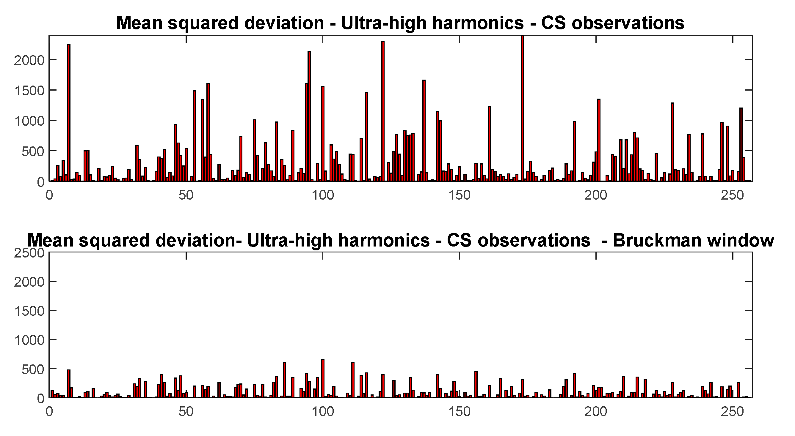
Next, let us examine the anti-interference performance of the signal with the addition of a Blackman window. Figure 3 shows the ultra-high-order harmonics and the ultra-high-order harmonics with the Blackman window applied. The horizontal axis represents the number of observed sampling points, and the vertical axis represents the mean square error. By comparing the mean square error of the observations using CS, it is evident that after applying the Blackman window, the mean square error decreases. This indicates that the energy fluctuation of the observed signal is reduced, making the signal more stable and its anti-interference capability stronger.

5.2. Analysis of the Accuracy of Ultra-High Harmonic Signal Reconstruction

In order to analyze the effect of the signal compression sampling method based on window function and compressed sensing proposed in this paper on the reconstruction of ultra-high harmonics in electrical energy signals, the performance evaluation indexes in Equations (21)–(23) are used in this paper to evaluate the effect, including reconstruction error $err$, mean square error percentage $MSE$ reconstruction signal-to-noise ratio $SNR$, where ${‖\cdot ‖}_2$ is the 2-norm and $N$ is the total signal length.

$$err=\frac{{‖\widehat{x}-x‖}_2}{{‖x‖}_2}\times 100\%$$

(21)

$$MSE={‖\widehat{x}-x‖}_2/N$$

(22)

$$SNR=10log\left({‖\widehat{x}‖}_2^2/MSE\right)dB$$

(23)

Below, we compare the reconstruction of ultra-high-order harmonics based on window functions and compressed sensing. First, we construct a compressed sensing sampling model for ultra-high-order harmonics. The observation target remains the ultra-high-order harmonics, with the measurement matrix being a Gaussian random matrix. The observation sample size $M$ is 256, the signal length $N$ is 400, the number of iterations $r$ is 128, and the sparsity $k$ is 64. It is known that harmonics exhibit good sparsity under the Discrete Fourier Transform (DFT); hence, the DFT is used as the sparse basis Ψ, and the Orthogonal Matching Pursuit (OMP) algorithm is employed for reconstruction. CS reconstructions of ultra-high-order harmonics are performed both without windowing and with the addition of five different window functions, and the results are compared. The evaluation of reconstruction effects is shown in

Table 4. Comparison of the reconstruction effects of CS and adding different window functions.

Window Function	$\mathit{e}\mathit{r}\mathit{r}$	$\mathit{M}\mathit{S}\mathit{E}$	$\mathit{S}\mathit{N}\mathit{R}(\mathbf{dB})$
CS	5.15 × 10−2	3.60 × 10−2	63.39
Rectangular Window + CS	6.10 × 10−2	4.26 × 10−2	62.61
Taylor Window + CS	1.91 × 10−2	1.46 × 10−2	68.08
Hamming Window + CS	6.91 × 10−3	3.08 × 10−3	70.14
Bartlett Window + CS	1.07 × 10−3	4.35 × 10−4	77.83
Blackman Window + CS	4.15 × 10−6	4.13 × 10−6	97.69

. The data in Table 4 indicate that the reconstruction values of the CS signal and the rectangular window + CS signal are slightly different, due to the measurement matrix generating a new Gaussian matrix for each observation and reconstruction. However, their overall reconstruction effects are essentially similar. For the Taylor, Hamming, and Bartlett windows + CS signals, the reconstruction error and mean square error (MSE) percentages are reduced to varying degrees, and the signal-to-noise ratio (SNR) increases accordingly, indicating improved reconstruction effects. Notably, the Blackman window + CS has the best reconstruction effect. This is because adding windows increases the sparsity of ultra-high-order harmonics in the DFT domain, and the sparser the signal, the better the reconstruction effect. In Table 4, the reconstruction accuracies of the windowed signals are ranked from low to high as follows: rectangular window, Taylor window, Hamming window, Bartlett window, and Blackman window. This ranking is consistent with the analysis of the sparsity distribution of the windowed signals in Figure 2 and Table 1. Specifically, after adding the Blackman window, the signal’s sparsity is optimized, and the energy distribution after observation is most concentrated, leading to the best reconstruction effect.

Adding the Blackman window for CS reconstruction significantly improves the reconstruction effect compared to CS reconstruction alone. The reconstruction error and MSE percentages are reduced from ${10}^{-2}$ to ${10}^{-6}$, and the reconstruction SNR is increased by 34.3 dB to 97.69 dB, an improvement of 54.11%. This demonstrates that the Blackman window is highly effective in reducing the spectral leakage of ultra-high-order harmonic signals. The addition of the Blackman window maximizes the preservation of ultra-high-order harmonic information and eliminates spectral leakage while enhancing signal sparsity, fully meeting the requirements for monitoring power quality.

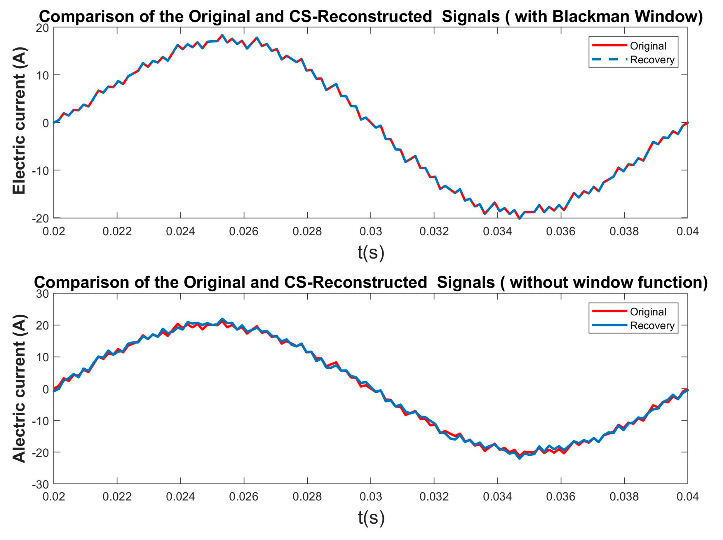
The ultra-high-order harmonic signals were reconstructed separately after compressed sensing alone and after Blackman windowing combined with compressed sensing. The comparison between the twice reconstructed signals and the original signal is shown in Figure 4. In the figure, the horizontal axis represents time, and the vertical axis represents the waveform of the current signal over time. It can be observed that when reconstructing the ultra-high-order harmonic signals using compressed sensing without windowing, there is a noticeable discrepancy in the details between the reconstructed signal and the original signal. However, after applying the Blackman window function, the reconstructed signal is visually indistinguishable from the original signal, indicating that there is virtually no error between them. This demonstrates that the inclusion of the Blackman window significantly enhances the effectiveness of the reconstructed signal.

5.3. Effect of Compression Ratio on Window Function and Reconstruction Effect

This sub-section analyzes the effects of different compression ratios on window functions and reconstruction effects.

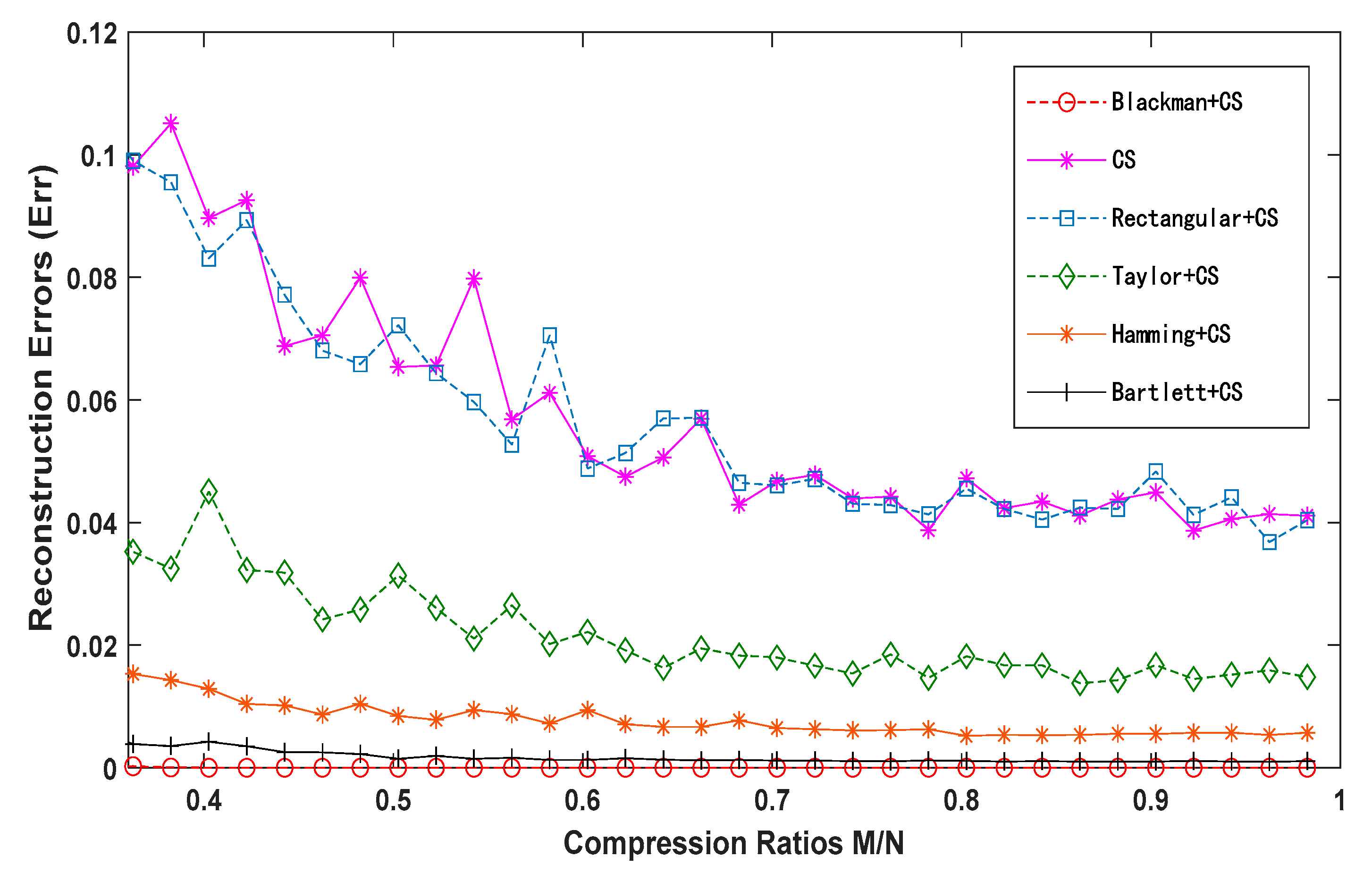
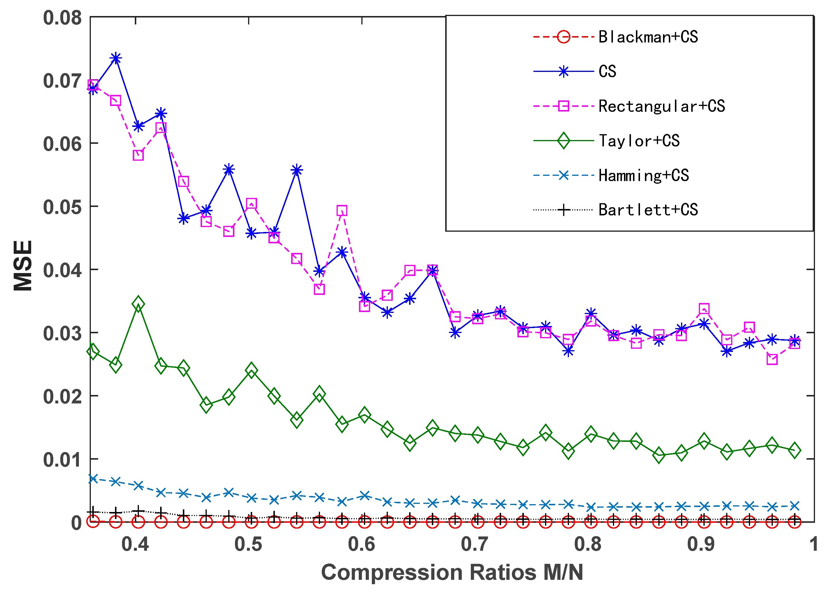
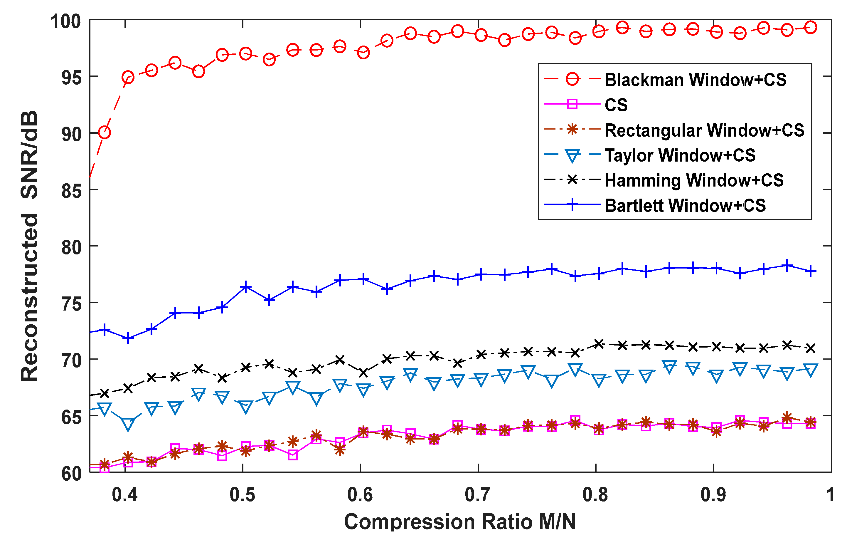
According to the principle of compressed sensing, the number of samples should satisfy Equation (4) to accurately reconstruct the signal. Based on the calculations, the compression ratio is set within a specific measurement range. Various compression ratios are employed for signal processing and reconstruction under different conditions, including compressed sensing reconstruction without windowing and with different window functions. The reconstructed results, R1, R2, and R3, are shown in Figure 5, Figure 6 and Figure 7, respectively, where the horizontal axis represents the compression ratio. In the general compressed sensing algorithm, for a given R, a higher compression ratio implies a larger number of samples M, which, in turn, means that more information from the original signal is contained in the observation vector Y, resulting in a better reconstruction effect. From the trends observed in Figure 5, Figure 6 and Figure 7, it is evident that the reconstruction effects of window function + CS observations improve with an increasing compression ratio. This is consistent with the general relationship between the reconstruction effect and the compression ratio in the compression-aware algorithm. Adding the rectangular window does not alter the reconstruction effect of ultra-high-order harmonics; the results are essentially the same as those of CS reconstruction without any window. However, after applying the Taylor, Hamming, Bartlett, and Blackman windows, the reconstruction accuracy significantly improves for the same compression ratio. Among these, the Blackman window yields the best reconstruction effect. These simulation results align with the analysis of the reconstruction data presented in Table 4.

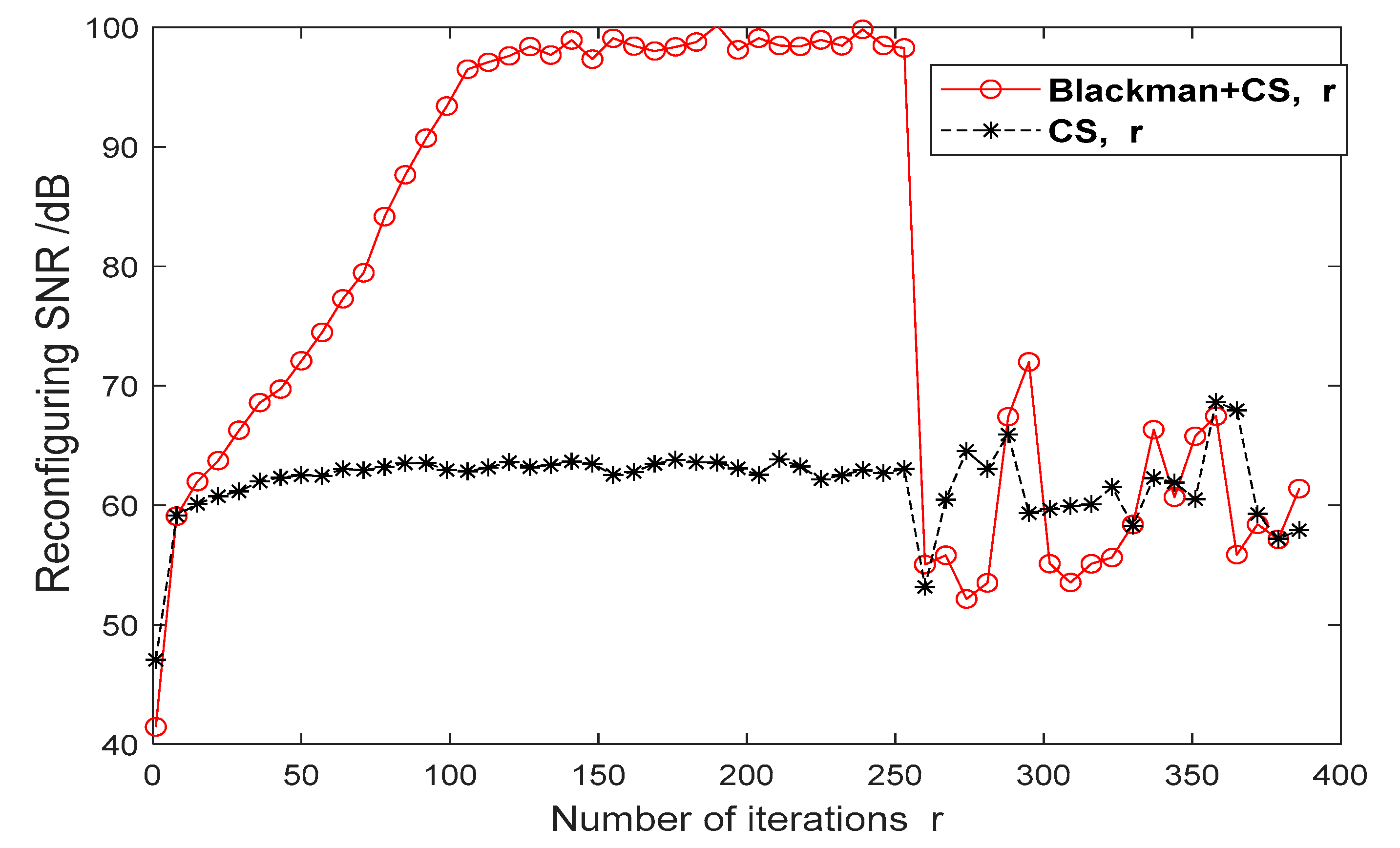
5.4. Effect of the Number of Iterations on the Window Function and Reconstruction Effect

In this sub-section, the effect of the number of CS iterations $r$ on the signal reconstruction is analyzed. The window function that performed best in the discussion above, the Blackman window, is selected for this investigation. The signal length $N$ = 400, $M$ = 256, and OMP algorithm is adopted as the recovery algorithm, and the signal reconstruction effect is shown in Figure 8. It can be seen that the CS reconstruction signal-to-noise ratio is not affected by the number of iterations for the number of iterations within $20<r<260$ in the case without a window. However, if the Blackman window is added, the reconstruction signal-to-noise ratio may be improved significantly if the number of iterations is kept within $110<r<260$. In this range, the change in the number of iterations has generally no effect on the signal reconstruction.

6. Results

Due to the widespread deployment of high-proportion power electronic devices, the ultra-high-order harmonic components in the range of 2 kHz to 150 kHz in distribution networks have significantly increased. The application of compressed sensing algorithms to process these ultra-high-order harmonics is challenged by considerable spectral leakage. This paper presents a novel observation method for ultra-high-order harmonics that combines window functions with compressed sensing. Through a detailed analysis of signal sparsity, the Blackman window function has been identified as the most suitable for both the compressed sensing reconstruction process and the specific characteristics of ultra-high-order harmonics.

Simulation results demonstrate that, in comparison to the sole application of the compressed sensing algorithm, the proposed method—integrating the Blackman window with compressed sensing—yields a more sparse observed signal, reduces energy fluctuations, enhances robustness, and improves anti-interference capability. The reconstruction error (ERR) and mean square error (MSE) percentage decrease from ${10}^{-2}$ to ${10}^{-6}$, and the reconstruction signal-to-noise ratio (SNR) increases by 34.3 dB, achieving 97.69 dB, an improvement of 54.11%. These results indicate a significant enhancement in reconstruction performance. This study provides new theoretical insights and methodologies for the analysis and processing of ultra-high-order harmonics induced by high-proportion power electronic devices.

In this study, the measurement matrix for compressed sensing was chosen as a universal Gaussian random matrix, without designing a specific measurement matrix tailored to the characteristics of ultra-high-order harmonics. In future work, based on the algorithm presented in this paper, we will extract the mathematical features of ultra-high-order harmonics to design corresponding measurement matrices. Additionally, we will further optimize the recovery algorithm to enhance the practical application of compressed sensing in the processing of ultra-high-order harmonic data.

References

- Bai, J.; Xin, S.; Liu, J.; Zheng, K. Research on the development path of high proportion of renewable energy in China. Proc. CSEE 2015, 35, 3699–3705. [Google Scholar]
- Lu, Z.; Li, H.; Qiao, Y. Evaluation and balance mechanism of power system flexibility for high-ratio renewable energy grid-connected. Proc. CSEE 2018, 38, 1893–1904. [Google Scholar]
- Zhou, X.; Chen, S.; Lu, Z.; Huang, Y.; Ma, S.; Zhao, Q. Technical characteristics of China’s new generation power system in energy transition. Proc. CSEE 2018, 38, 1893–1904. [Google Scholar]
- Feng, Y. The problem of ultra-high harmonics and its research status and trend. J. Electroacoust. Technol. 2018, 42, 33–34. [Google Scholar]
- Xiao, X.; Liao, K.; Tang, S.; Fan, W. Development of power electronicization and new problems of ultra-high harmonics in distribution network. Trans. China Electrotech. Soc. 2018, 33, 707–720. [Google Scholar]
- Lin, H. New Development of Harmonic Problems in No.4 Power Grid-Talking about Superharmonics. Power Supply 2016, 33, 35–38. [Google Scholar]
- Liu, S.; Huang, B.; Wang, C. Overview of super harmonic research. Electr. Meas. Insturmentation. 2017, 54, 7–15. [Google Scholar]
- Moreno-Munoz, A.; Gil-de-Castro, A.; Romero-Cavadal, E.; Rönnberg, S.; Bollen, M. Supraharmonics (2 to 150 kHz) and multi-level converters. In Proceedings of the 2015 IEEE 5th International Conference on Power Engineering, Energy and Electrical Drives (POWERENG), Riga, Latvia, 11–13 May 2015. [Google Scholar]
- Meyer, J.; Blanco, A.-M.; Rönnberg, S.; Bollen, M.; Smith, J. CIGRE C4/C6.29: Survey of utilities experiences on power quality issues related to solar power. CIRED-Open Access Proc. J. 2017, 2017, 539–543. [Google Scholar] [CrossRef]
- Rönnberg, S.; Bollen, M. Power quality issues in the electric power system of the future. Electr. J. 2016, 29, 49–61. [Google Scholar] [CrossRef]
- Rönnberg, S.K.; Castro, A.G.; Moreno-Munoz, A.; Bollen, M.H.J.; Garrido, J. Solar PV inverter supraharmonics reduction with random PWM. In Proceedings of the 2017 11th IEEE International Conference on Compatibility, Power Electronics and Power Engineering (CPE-POWERENG), Cadiz, Spain, 4–6 April 2017. [Google Scholar]
- Subhani, S.; Cuk, V.; Cobben, J.F.G. A literature survey on power quality disturbances in the frequency range of 2-150 kHz. Renew. Energy Power Qual. J. 2017, 1, 405–410. [Google Scholar] [CrossRef]
- Waniek, C.; Wohlfahrt, T.; Myrzik, J.M.A.; Meyer, J.; Klatt, M.; Schegner, P. Supraharmonics: Root causes and interactions between multiple devices and the low voltage grid. In Proceedings of the 2017 IEEE PES Innovative Smart Grid Technologies Conference Europe (ISGT-Europe), Turin, Italy, 26–29 September 2017; Volume 17520385. [Google Scholar]
- Kalesar, B.M.; Noshahr, J.B. Capacitor bank behaviour of cement factory in presence of supra-harmonics resulted from switching full-power frequency converter of generator. CIRED-Open Access Proc. J. 2017, 2017, 535–538. [Google Scholar] [CrossRef]
- Grevener, A.; Meyer, J.; Rönnberg, S.; Bollen, M.; Myrzik, J. Survey of supraharmonic emission of household appliances. CIRED-Open Access Proc. J. 2017, 2017, 535–538. [Google Scholar] [CrossRef]
- Liu, Q.; Zhang, J.; Lin, F.; Xu, F.; Zhang, W. A Method for Supraharmonic Source Determination Based on Complex ICA. In Proceedings of the 2018 China International Conference on Electricity Distribution (CICED), Tianjin, China, 17–19 September 2018. [Google Scholar]
- Körner, P.M.; Stiegler, R.; Meyer, J.; Wohlfahrt, T.; Waniek, C.; Myrzik, J.M.A. Acoustic noise of massmarket equipment caused by supraharmonics in the frequency range 2 to 20 kHz. In Proceedings of the 2018 18th International Conference on Harmonics and Quality of Power (ICHQP), Ljubljana, Slovenia, 13–16 May 2018. [Google Scholar]
- Meyer, J.; Bollen, M.; Amaris, H.; Blanco, A.M.; de Castro, A.G.; Desmet, J.; Klatt, M.; Kocewiak, Ł.; Rönnberg, S.; Yang, K. Future work on harmonics—Some expert opinions Part II—Supraharmonics, standards and measurements. In Proceedings of the 2014 16th International Conference on Harmonics and Quality of Power (ICHQP), Bucharest, Romania, 25–28 May 2014. [Google Scholar]
- Yalcin, T.; Özdemir, M.; Kostyla, P.; Leonowicz, Z. Analysis of supra-harmonics in smart grids. In Proceedings of the 2017 IEEE International Conference on Environment and Electrical Engineering and 2017 IEEE Industrial and Commercial Power Systems Europe (EEEIC/I&CPS Europe), Milan, Italy, 6–9 June 2017. [Google Scholar]
- Rodrigues, C.E.M.; de Lima Tostes, M.E. Characterization of supraharmonics using the wavelet packet transform. In Proceedings of the 2018 18th International Conference on Harmonics and Quality of Power (ICHQP), Ljubljana, Slovenia, 13–16 May 2018. [Google Scholar]
- Mendes, T.M.; Duque, C.A.; Silva, L.R.M.; Ferreira, D.D.; Ribeiro, P.F.; Meyer, J.; Grevener, A. Supraharmonic analysis using subsampling. In Proceedings of the 2018 18th International Conference on Harmonics and Quality of Power (ICHQP), Ljubljana, Slovenia, 13–16 May 2018. [Google Scholar]
- Zhuang, S.; Zhao, W.; Wang, R.; Wang, Q.; Huang, S. New Measurement Algorithm for Supraharmonics Based on Multiple Measurement Vectors Model and Orthogonal Matching Pursuit. IEEE Trans. Instrum. Meas. 2019, 68, 1671–1679. [Google Scholar] [CrossRef]
- Larsson, E.O.A.; Bollen, M.H.J.; Wahlberg, M.G.; Lundmark, C.M.; Ronnberg, S.K. Measurements of High-Frequency (2–150 kHz) Distortion in Low-Voltage Networks. IEEE Trans. Power Deliv. 2010, 25, 1749–1757. [Google Scholar] [CrossRef]
- Huang, C.; Jiang, Y.-Q. Improved Windowing Interpolation Algorithm for Harmonic Analysis. Proc. CSEE 2005, 25, 26–32. [Google Scholar]
- Ting, Y.; Jincheng, W.; Yuan, B. The Restoration Algorithm of Compressed Sensing to Detect Harmonic and Inter-harmonic. Proc. CSEE 2015, 35, 5475–5482. [Google Scholar]
- Donoho, D. Compressed sensing. IEEE Trans. Inf. Theory 2006, 52, 1289–1306. [Google Scholar] [CrossRef]