
Fast Depth Map Coding Algorithm for 3D-HEVC Based on Gradient Boosting Machine


Abstract
1. Introduction
2. Related Work
3. Proposed Algorithm
3.1. GBM-Based Adaptive CU Partition
3.1.1. Observations and Analysis
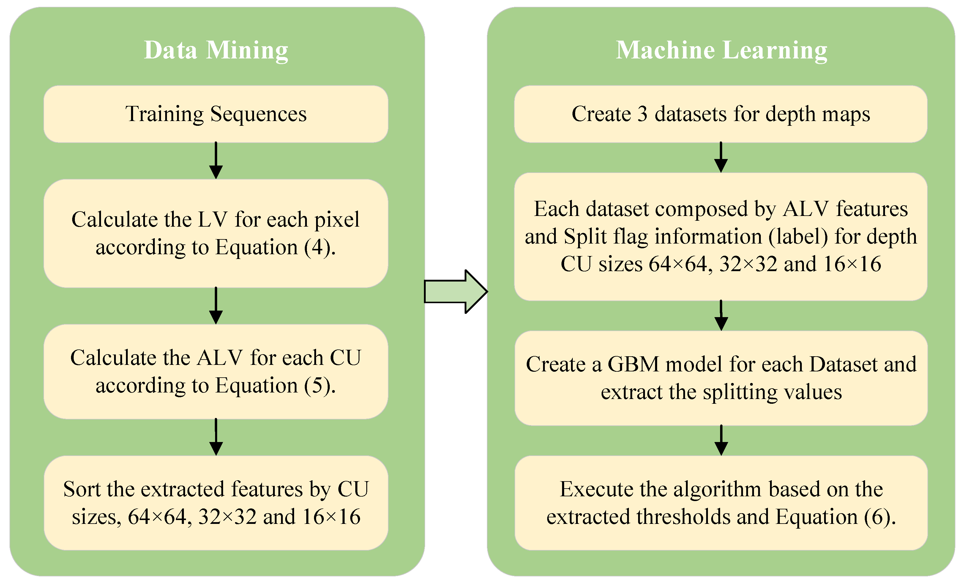
3.1.2. Gradient Boosting Machines Algorithm
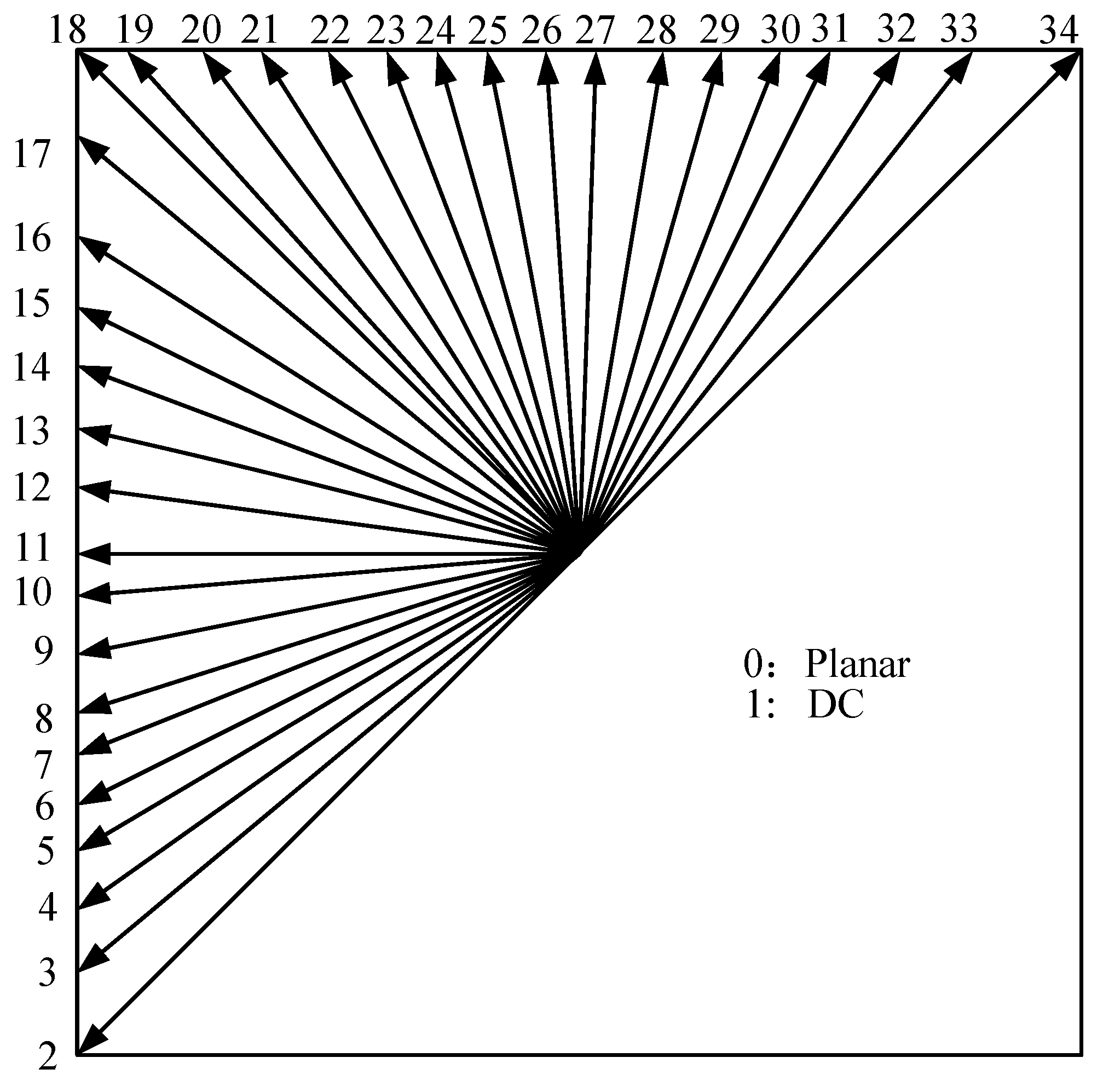
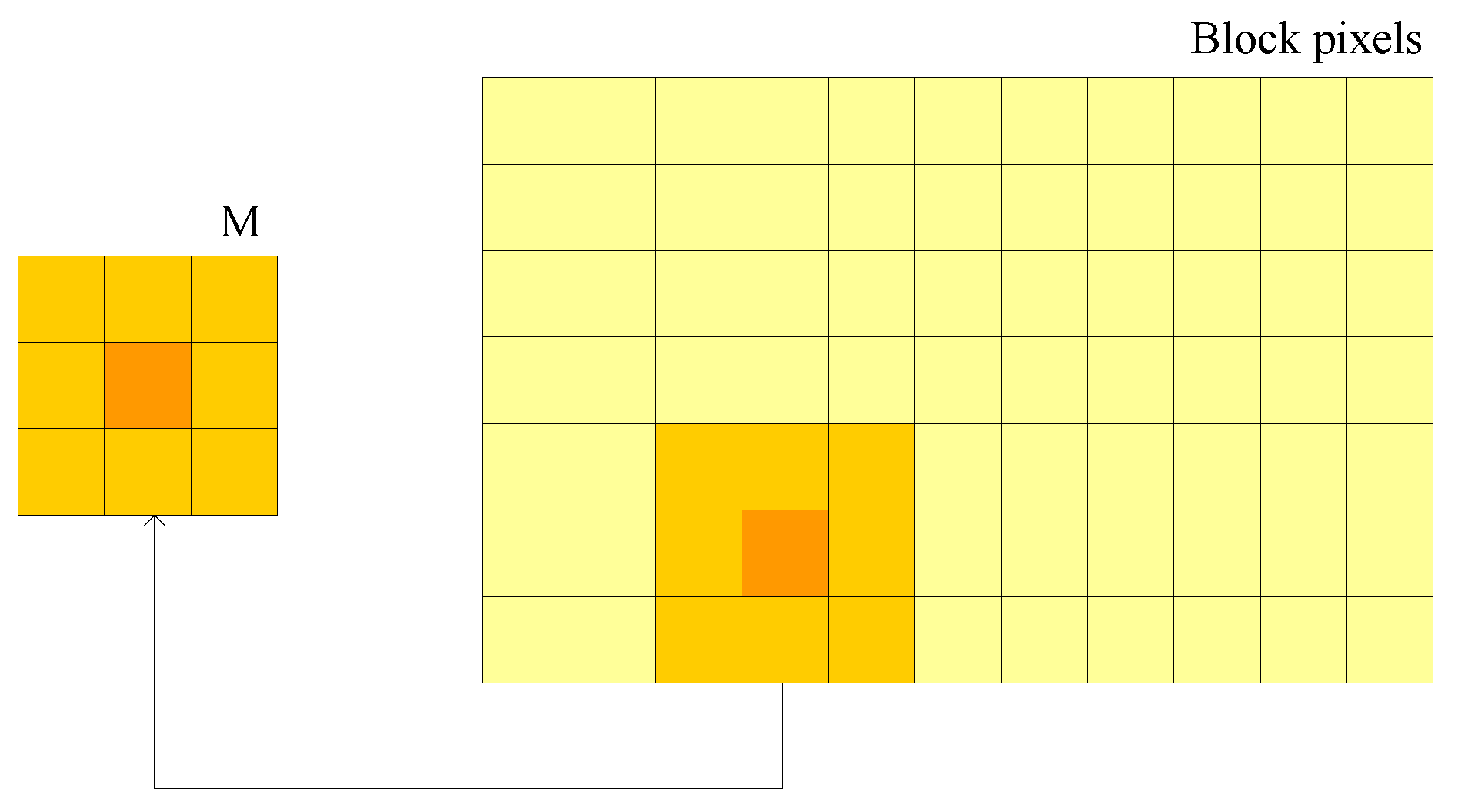
3.1.3. Feature Selection and Adaptive CU Size Decision Algorithm
3.2. Fast Rate–Distortion-Optimization Algorithm
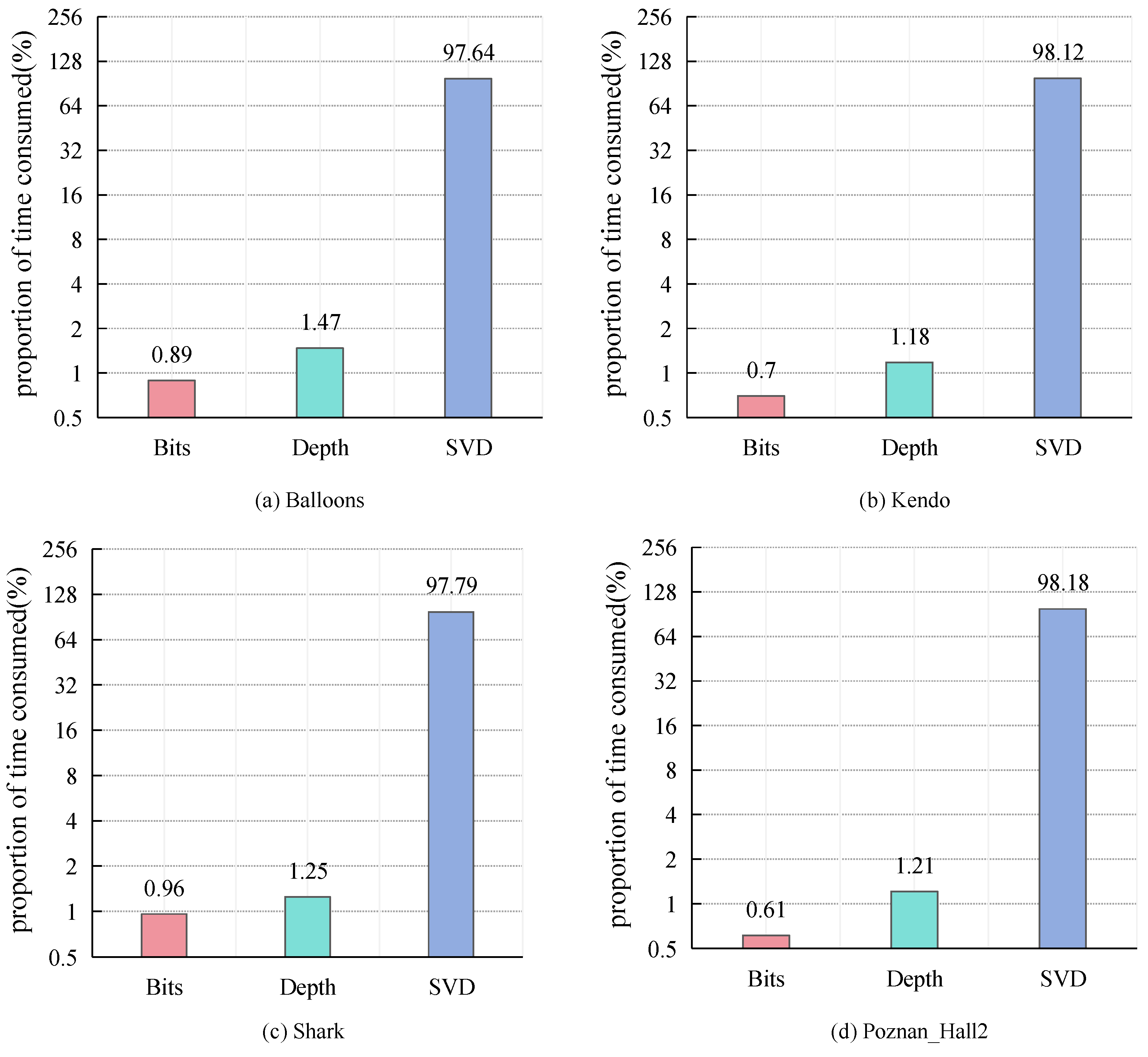
3.2.1. Observations and Analysis
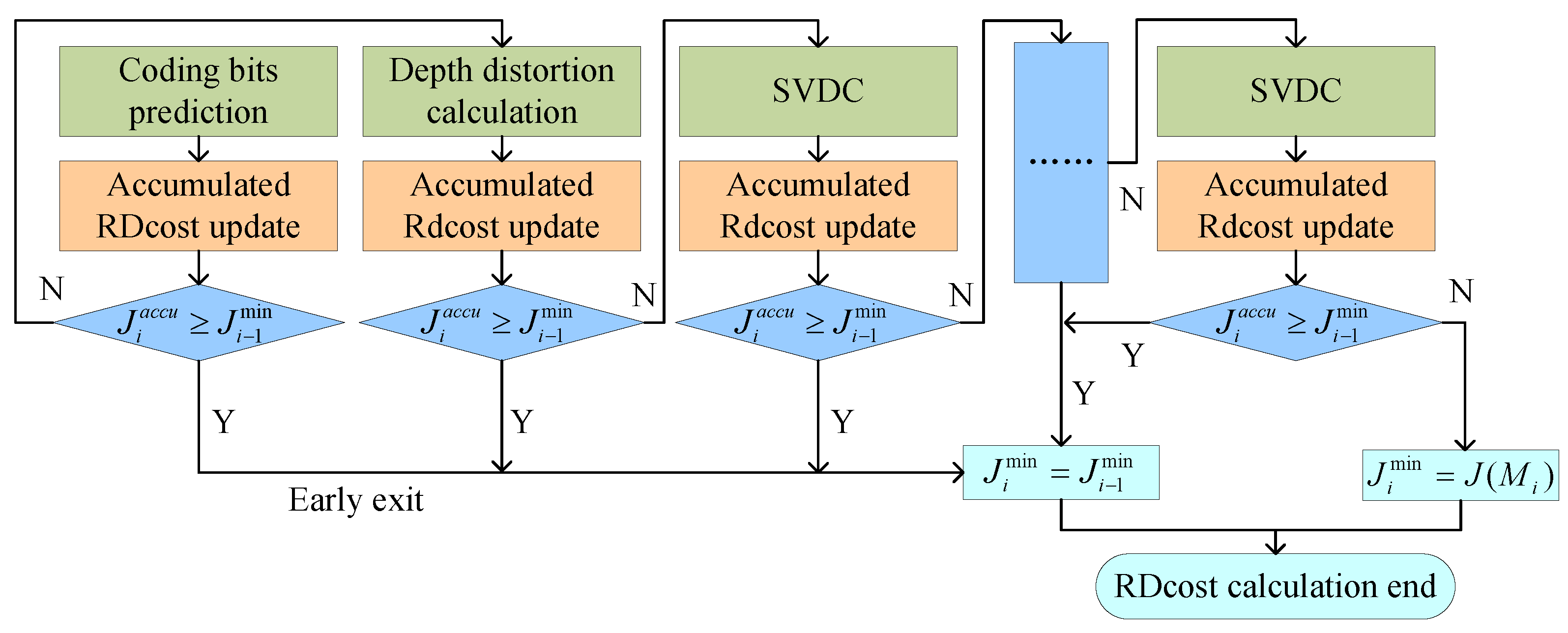
3.2.2. RDO Process
4. Experimental Results
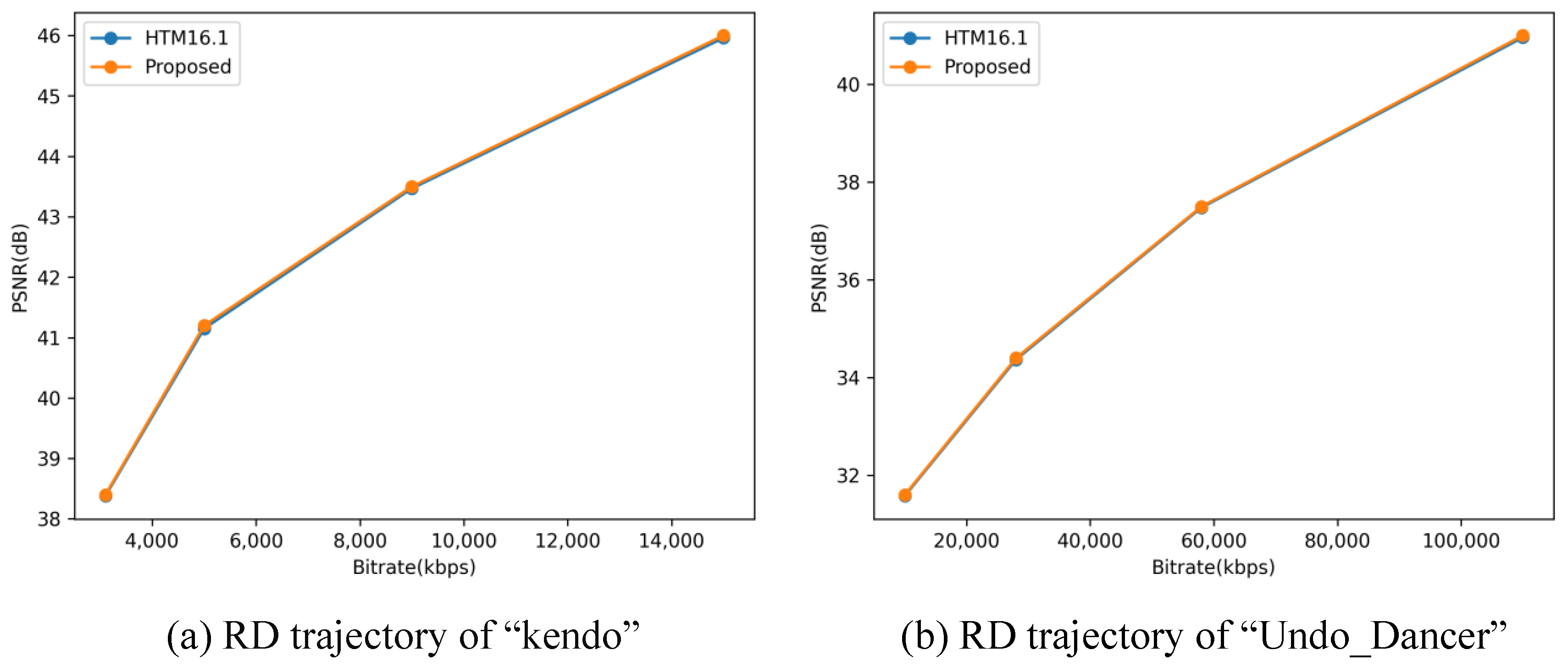
4.1. Analysis of Experimental Results
4.2. Comparison with Other Algorithms
4.3. Discussion
5. Conclusions
Author Contributions
Funding
Data Availability Statement
Conflicts of Interest
References
- Müller, K.; Merkle, P.; Wiegand, T. 3-D video representation using depth maps. Proc. IEEE 2010, 99, 643–656. [Google Scholar] [CrossRef]
- Chen, Y.; Vetro, A. Next-generation 3D formats with depth map support. IEEE Multimed. 2014, 21, 90–94. [Google Scholar] [CrossRef]
- Tech, G.; Chen, Y.; Müller, K.; Ohm, J.R.; Vetro, A.; Wang, Y.K. Overview of the multiview and 3D extensions of high efficiency video coding. IEEE Trans. Circuits Syst. Video Technol. 2015, 26, 35–49. [Google Scholar] [CrossRef]
- Boyce, J.M.; Doré, R.; Dziembowski, A.; Fleureau, J.; Jung, J.; Kroon, B.; Salahieh, B.; Vadakital, V.K.M.; Yu, L. MPEG Immersive Video Coding Standard. Proc. IEEE 2021, 109, 1521–1536. [Google Scholar] [CrossRef]
- Paul, M. Efficient Multiview Video Coding Using 3-D Coding and Saliency-Based Bit Allocation. IEEE Trans. Broadcast. 2018, 64, 235–246. [Google Scholar] [CrossRef]
- Zhu, C.; Li, S.; Zheng, J.; Gao, Y.; Yu, L. Texture-Aware Depth Prediction in 3D Video Coding. IEEE Trans. Broadcast. 2016, 62, 482–486. [Google Scholar] [CrossRef]
- Alatan, A.A.; Yemez, Y.; Gudukbay, U.; Zabulis, X.; Muller, K.; Erdem, C.E.; Weigel, C.; Smolic, A. Scene Representation Technologies for 3DTV—A Survey. IEEE Trans. Circuits Syst. Video Technol. 2007, 17, 1587–1605. [Google Scholar] [CrossRef]
- Fehn, C. Depth-image-based rendering (DIBR), compression, and transmission for a new approach on 3D-TV. In Proceedings of the Stereoscopic Displays and Virtual Reality Systems XI, San Jose, CA, USA, 18–22 January 2004; Volume 5291, pp. 93–104. [Google Scholar]
- Zhang, Q.; Li, N.; Huang, L.; Gan, Y. Effective early termination algorithm for depth map intra coding in 3D-HEVC. Electron. Lett. 2014, 50, 994–996. [Google Scholar] [CrossRef]
- Sullivan, G.J.; Ohm, J.R.; Han, W.J.; Wiegand, T. Overview of the High Efficiency Video Coding (HEVC) Standard. IEEE Trans. Circuits Syst. Video Technol. 2012, 22, 1649–1668. [Google Scholar] [CrossRef]
- Liu, H.; Chen, Y. Generic segment-wise DC for 3D-HEVC depth intra coding. In Proceedings of the 2014 IEEE International Conference on Image Processing (ICIP), Paris, France, 27–30 October 2014; pp. 3219–3222. [Google Scholar] [CrossRef]
- Bakkouri, S.; Elyousfi, A. An adaptive CU size decision algorithm based on gradient boosting machines for 3D-HEVC inter-coding. Multimed. Tools Appl. 2023, 82, 32539–32557. [Google Scholar] [CrossRef]
- Li, Y.; Yang, G.; Zhu, Y.; Ding, X.; Sun, X. Adaptive Inter CU Depth Decision for HEVC Using Optimal Selection Model and Encoding Parameters. IEEE Trans. Broadcast. 2017, 63, 535–546. [Google Scholar] [CrossRef]
- Lei, J.; Duan, J.; Wu, F.; Ling, N.; Hou, C. Fast Mode Decision Based on Grayscale Similarity and Inter-View Correlation for Depth Map Coding in 3D-HEVC. IEEE Trans. Circuits Syst. Video Technol. 2018, 28, 706–718. [Google Scholar] [CrossRef]
- Huo, J.; Zhou, X.; Yuan, H.; Wan, S.; Yang, F. Fast Rate-Distortion Optimization for Depth Maps in 3-D Video Coding. IEEE Trans. Broadcast. 2023, 69, 21–32. [Google Scholar] [CrossRef]
- Oh, B.T.; Oh, K.J. View Synthesis Distortion Estimation for AVC- and HEVC-Compatible 3-D Video Coding. IEEE Trans. Circuits Syst. Video Technol. 2014, 24, 1006–1015. [Google Scholar] [CrossRef]
- Saldanha, M.; Sanchez, G.; Marcon, C.; Agostini, L. Fast 3D-HEVC Depth Map Encoding Using Machine Learning. IEEE Trans. Circuits Syst. Video Technol. 2020, 30, 850–861. [Google Scholar] [CrossRef]
- Bakkouri, S.; Elyousfi, A. Early Termination of CU Partition Based on Boosting Neural Network for 3D-HEVC Inter-Coding. IEEE Access 2022, 10, 13870–13883. [Google Scholar] [CrossRef]
- Bakkouri, S.; Elyousfi, A.; Hamout, H. Fast CU size and mode decision algorithm for 3D-HEVC intercoding. Multimed. Tools Appl. 2020, 79, 6987–7004. [Google Scholar] [CrossRef]
- Zou, D.; Dai, P.; Zhang, Q. Fast Depth Map Coding Based on Bayesian Decision Theorem for 3D-HEVC. IEEE Access 2022, 10, 51120–51127. [Google Scholar] [CrossRef]
- Li, Y.; Yang, G.; Qu, A.; Zhu, Y. Tunable early CU size decision for depth map intra coding in 3D-HEVC using unsupervised learning. Digit. Signal Process. 2022, 123, 103448. [Google Scholar] [CrossRef]
- Wang, X. Application of 3D-HEVC fast coding by Internet of Things data in intelligent decision. J. Supercomput. 2022, 78, 7489–7508. [Google Scholar] [CrossRef]
- Chen, J.; Wang, B.; Liao, J.; Cai, C. Fast 3D-HEVC inter mode decision algorithm based on the texture correlation of viewpoints. Multimed. Tools Appl. 2019, 78, 29291–29305. [Google Scholar] [CrossRef]
- Shen, L.; Li, K.; Feng, G.; An, P.; Liu, Z. Efficient Intra Mode Selection for Depth-Map Coding Utilizing Spatiotemporal, Inter-Component and Inter-View Correlations in 3D-HEVC. IEEE Trans. Image Process. 2018, 27, 4195–4206. [Google Scholar] [CrossRef] [PubMed]
- Song, W.; Dai, P.; Zhang, Q. Content-adaptive mode decision for low complexity 3D-HEVC. Multimed. Tools Appl. 2023, 82, 26435–26450. [Google Scholar] [CrossRef]
- Zhang, Z.; Yu, L.; Qian, J.; Wang, H. Learning-Based Fast Depth Inter Coding for 3D-HEVC via XGBoost. In Proceedings of the 2022 Data Compression Conference (DCC), Snowbird, UT, USA, 22–25 March 2022; pp. 43–52. [Google Scholar] [CrossRef]
- Bentéjac, C.; Csörgo, A.; Martínez-Muñoz, G. A comparative analysis of gradient boosting algorithms. Artif. Intell. Rev. 2021, 54, 1937–1967. [Google Scholar] [CrossRef]
- Ali, Z.A.; Abduljabbar, Z.H.; Taher, H.A.; Sallow, A.B.; Almufti, S.M. Exploring the power of eXtreme gradient boosting algorithm in machine learning: A review. Acad. J. Nawroz Univ. 2023, 12, 320–334. [Google Scholar]
- Lu, H.; Karimireddy, S.P.; Ponomareva, N.; Mirrokni, V. Accelerating gradient boosting machines. In Proceedings of the International Conference on Artificial Intelligence and Statistics, Online, 26–28 August 2020; pp. 516–526. [Google Scholar]
- Hamout, H.; Elyousfi, A. Fast 3D-HEVC PU size decision algorithm for depth map intra-video coding. J. Real-Time Image Process. 2020, 17, 1285–1299. [Google Scholar] [CrossRef]
- Tung, L.V.; Le Dinh, M.; HoangVan, X.; Dinh, T.D.; Vu, T.H.; Le, H.T. View synthesis method for 3D video coding based on temporal and inter view correlation. IET Image Processing 2018, 12, 2111–2118. [Google Scholar] [CrossRef]


| Sequence | QP | Depth 0 (%) | Depth 1 (%) | Depth 2 (%) | Depth 3 (%) |
|---|---|---|---|---|---|
| Kendo | 34 | 87.83 | 8.94 | 2.34 | 0.89 |
| 39 | 94.06 | 5.14 | 0.78 | 0.02 | |
| 42 | 96.97 | 2.73 | 0.29 | 0.01 | |
| 45 | 98.89 | 0.98 | 0.13 | 0.00 | |
| Balloons | 34 | 84.98 | 10.60 | 4.19 | 0.23 |
| 39 | 96.06 | 2.94 | 0.93 | 0.07 | |
| 42 | 98.17 | 1.39 | 0.42 | 0.02 | |
| 45 | 98.82 | 1.06 | 0.11 | 0.01 | |
| Shark | 34 | 82.58 | 11.13 | 5.74 | 0.55 |
| 39 | 92.98 | 5.77 | 1.04 | 0.21 | |
| 42 | 97.27 | 2.36 | 0.32 | 0.05 | |
| 45 | 99.13 | 0.73 | 0.13 | 0.01 | |
| Poznan_Hall2 | 34 | 96.47 | 2.48 | 1.05 | 0.00 |
| 39 | 98.96 | 0.92 | 0.12 | 0.00 | |
| 42 | 99.72 | 0.25 | 0.03 | 0.00 | |
| 45 | 99.93 | 0.05 | 0.02 | 0.00 | |
| Average | 95.18 | 3.59 | 1.10 | 0.13 |
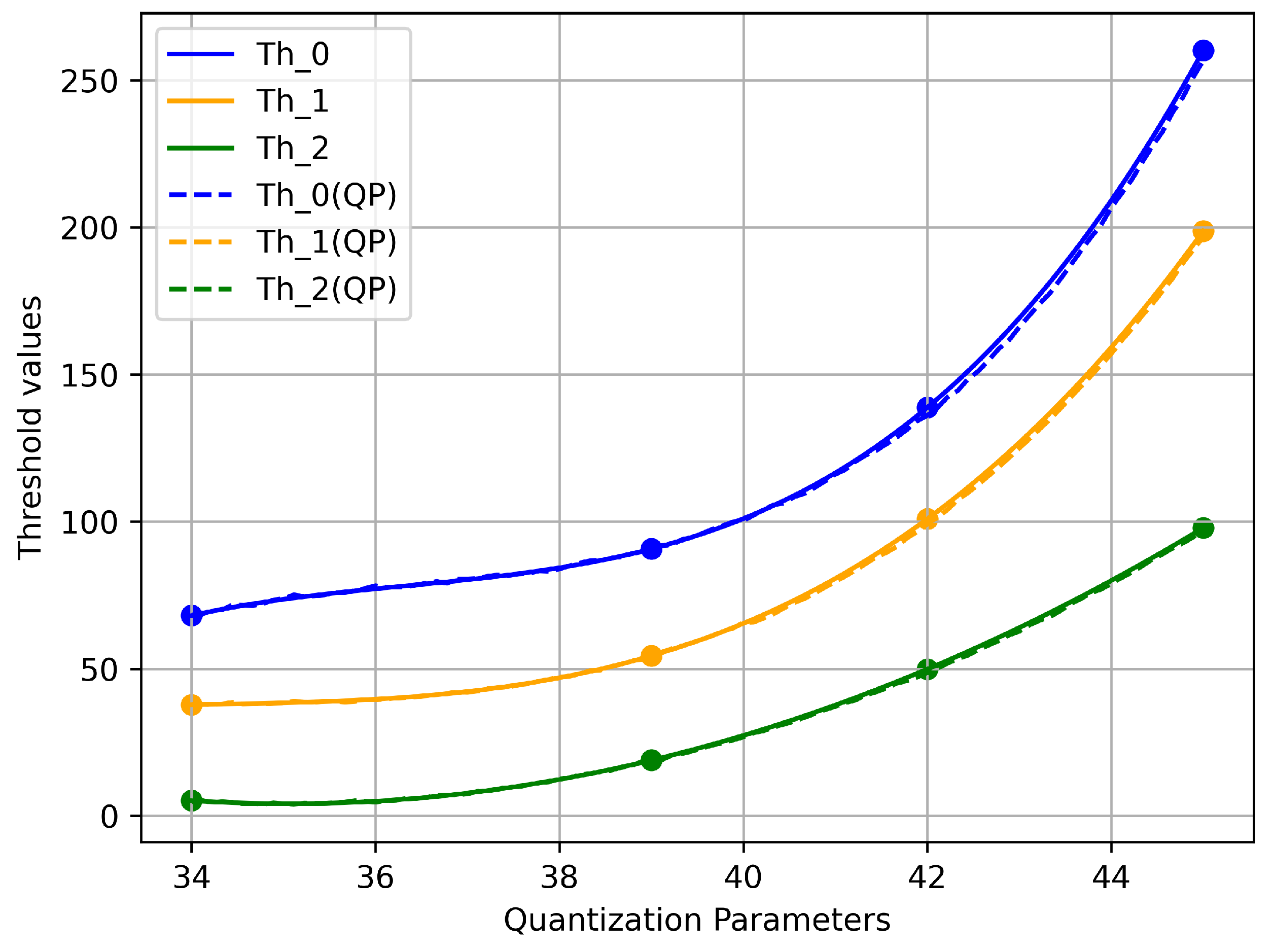
| QP | Thresholds | ||
|---|---|---|---|
| 34 | 68.0744 | 37.7616 | 5.1848 |
| 39 | 90.7334 | 54.3951 | 18.8968 |
| 42 | 138.7688 | 100.8912 | 49.8472 |
| 45 | 260.075 | 198.7125 | 97.84 |
| Sequence | Frames | Resolution |
|---|---|---|
| Balloons | 300 | 1024 × 768 |
| Newspaper | 300 | 1024 × 768 |
| Kendo | 300 | 1024 × 768 |
| GT_Fly | 250 | 1920 × 1088 |
| Shark | 300 | 1920 × 1088 |
| Poznan_Hall2 | 300 | 1920 × 1088 |
| Poznan_Street | 250 | 1920 × 1088 |
| Undo_Dancer | 250 | 1920 × 1088 |
| Sequence | BDBR (%) | BD-PSNR (db) | TS (%) | ||
|---|---|---|---|---|---|
| GBM | RDO | Overall | |||
| Kendo | 0.68 | −0.01 | 48.83 | 29.84 | 52.93 |
| Balloons | 0.83 | −0.02 | 44.57 | 33.75 | 49.82 |
| Newspaper | 0.89 | −0.03 | 47.68 | 34.58 | 53.38 |
| GT_Fly | 0.96 | −0.02 | 46.93 | 33.52 | 51.85 |
| Poznan_Hall2 | 1.27 | −0.01 | 45.06 | 29.64 | 52.37 |
| Poznan_Street | 1.08 | −0.01 | 46.71 | 28.43 | 49.85 |
| Undo_Dancer | 0.75 | −0.02 | 49.63 | 30.96 | 53.74 |
| Shark | 1.36 | −0.02 | 50.25 | 31.56 | 55.97 |
| Average | 0.98 | −0.02 | 47.46 | 31.54 | 52.49 |
| Sequence | Bakkouri [19] | Chen [23] | Zou [20] | Proposed | ||||
|---|---|---|---|---|---|---|---|---|
| BDBR (%) | TS (%) | BDBR (%) | TS (%) | BDBR (%) | TS (%) | BDBR (%) | TS (%) | |
| Balloons | 0.9 | 36.20 | 0.49 | 18.50 | 1.02 | 51.7 | 0.83 | 49.82 |
| Kendo | 1.10 | 34.80 | 0.18 | 19.40 | 1.09 | 52.2 | 0.68 | 52.93 |
| Newspaper | 0.55 | 31.80 | 0.04 | 14.10 | 1.21 | 49.8 | 0.89 | 53.38 |
| GT_Fly | 0.56 | 36.50 | −0.30 | 23.30 | 0.93 | 52.8 | 0.96 | 51.85 |
| Poznan_Hall2 | 0.50 | 36.30 | 0.46 | 26.30 | 0.65 | 57.1 | 1.27 | 52.37 |
| Poznan_Street | 0.60 | 30.00 | 0.20 | 15.80 | 0.85 | 53.4 | 1.08 | 49.85 |
| Undo_Dancer | 0.88 | 33.50 | 0.01 | 14.15 | 1.36 | 45.9 | 0.75 | 53.74 |
| Shark | 1.18 | 34.40 | 0.28 | 18.32 | 1.47 | 46.5 | 1.36 | 55.97 |
| Average | 0.78 | 34.19 | 0.17 | 18.73 | 1.07 | 51.20 | 0.98 | 52.49 |
Disclaimer/Publisher’s Note: The statements, opinions and data contained in all publications are solely those of the individual author(s) and contributor(s) and not of MDPI and/or the editor(s). MDPI and/or the editor(s) disclaim responsibility for any injury to people or property resulting from any ideas, methods, instructions or products referred to in the content. |
© 2024 by the authors. Licensee MDPI, Basel, Switzerland. This article is an open access article distributed under the terms and conditions of the Creative Commons Attribution (CC BY) license (https://creativecommons.org/licenses/by/4.0/).
Share and Cite
Su, X.; Liu, Y.; Zhang, Q. Fast Depth Map Coding Algorithm for 3D-HEVC Based on Gradient Boosting Machine. Electronics 2024, 13, 2586. https://doi.org/10.3390/electronics13132586
Su X, Liu Y, Zhang Q. Fast Depth Map Coding Algorithm for 3D-HEVC Based on Gradient Boosting Machine. Electronics. 2024; 13(13):2586. https://doi.org/10.3390/electronics13132586
Chicago/Turabian StyleSu, Xiaoke, Yaqiong Liu, and Qiuwen Zhang. 2024. "Fast Depth Map Coding Algorithm for 3D-HEVC Based on Gradient Boosting Machine" Electronics 13, no. 13: 2586. https://doi.org/10.3390/electronics13132586
APA StyleSu, X., Liu, Y., & Zhang, Q. (2024). Fast Depth Map Coding Algorithm for 3D-HEVC Based on Gradient Boosting Machine. Electronics, 13(13), 2586. https://doi.org/10.3390/electronics13132586