Abstract
Visibility is a measure of the atmospheric transparency at an observation point, expressed as the maximum horizontal distance over which a person can see and identify objects. Low atmospheric visibility often occurs in conjunction with air pollution, posing hazards to both traffic safety and human health. In this study, we combined satellite remote sensing images with environmental data to explore the classification performance of two distinct multimodal data processing techniques. The first approach involves developing four multimodal data classification models using deep learning. The second approach integrates deep learning and machine learning to create twelve multimodal data classifiers. Based on the results of a five-fold cross-validation experiment, the inclusion of various environmental data significantly enhances the classification performance of satellite imagery. Specifically, the test accuracy increased from 0.880 to 0.903 when using the deep learning multimodal fusion technique. Furthermore, when combining deep learning and machine learning for multimodal data processing, the test accuracy improved even further, reaching 0.978. Notably, weather conditions, as part of the environmental data, play a crucial role in enhancing visibility prediction performance.
1. Introduction
Visibility is a measure of the atmospheric transparency of an observation point, expressed as how far away horizontally a person can see and identify objects. Low atmospheric visibility is often accompanied by air pollution, which harms traffic safety and human health. The presence of atmospheric particles will always lead to reduced visibility [1], but low visibility does not directly mean poor air quality. Weather conditions and air quality are possible factors that affect atmospheric visibility. Effectively classifying and predicting visibility can significantly enhance safety and efficiency across multiple fields, reducing risks and losses associated with low-visibility conditions.
Exploring the relationships between features helps to identify key factors that influence classification. In 2005, Tsai explored the relationship between air pollution, meteorological parameters, and visibility using data from air quality monitoring stations [2]. In 2013, Zheng et al. used a spatial classifier based on artificial neural networks to investigate various factors that influence air quality [3]. Machine learning algorithms [4,5] have become a mature technology, and many studies use machine learning to perform classification tasks. In 2024, Sayed et al. utilized machine learning algorithms to classify learners based on their learning activity clicks. Their model predicted the most suitable evaluation strategies for each student with 98% accuracy using the random forest algorithm [5].
Many studies have confirmed that artificial neural networks, especially deep learning methods, can effectively perform visibility prediction. In 2017, Li et al. used a pre-trained convolutional neural network (CNN) to automatically extract visibility features, and a generalized regression neural network (GRNN) was designed for intelligent visibility evaluation based on these deep learning features [6]. In 2019, Ortega et al. used machine learning algorithms to classify visibility conditions into three categories based on weather station data in Florida. An artificial neural network achieved the highest average accuracy score [7]. Palvanov and Cho proposed a model named VisNet based on deep CNN to estimate visibility distances from camera imagery [8]. In 2020, Wang et al. proposed a CNN multimodal deep fusion architecture that used visible–infrared image pairs to estimate the visibility range [9]. In 2022, Liu et al. developed a deep integrated model using VGG-16 and Xception for airport visibility classification and analyzed influencing factors through a data-driven deep learning approach and multiple nonlinear regression analysis [10].
Research in recent years has confirmed that the multimodal technique can help improve prediction performance. In 2019, Zhang et al. established a multimodal fusion prediction system, estimating factory emissions through satellite images and training a fusion model for numerical regressions, effectively improving visibility prediction capabilities [11]. In 2021, Holste et al. compared different fusion strategies using DCE-MRI and clinical data from 10,185 breast MRI examinations. They demonstrated that integrating imaging and non-image clinical data significantly improved breast cancer classification performance, with models fusing intermediate features outperforming those fusing final probabilities [12]. To achieve the multimodal technique, image feature extraction is indispensable. By extracting key features from images, this technique provides the essential data foundation for multimodal approaches. These image features can be integrated with other modalities, enabling more comprehensive and accurate data analysis and decision making. Utilizing pre-trained deep learning models for automatic feature extraction from images has become a mature technique [13], as demonstrated by Hussain et al. [14] and Chang et al. [4] who employed transfer learning methods to obtain higher-level image features.
The purposes of this study are as follows:
- To combine satellite remote sensing images and environmental data to form a multimodal dataset, effectively improving the classification performance of visibility;
- To compare two different multimodal data processing techniques to establish the optimal visibility classification model;
- To investigate the impact of various environmental data features on multiclass visibility classification performance.
2. Materials and Methods
2.1. Materials
This study collected image data and environmental data to build a nationwide satellite multimodal dataset in Taiwan, covering the period from 12–18 December 2022. The data were collected from various counties and cities in Taiwan, encompassing a total of 19 different regions. For the image data, satellite remote sensing images from Google Earth/Google Maps [15] were utilized, with a size of 1280 × 1280 × 3 pixels. The environmental data contain three types of data, including geographical location, weather conditions, and air quality data. Geographical location data use population density as a classification feature and were collected from the Department of Household Registration of the Ministry of the Interior [16]; meteorological and air quality data were collected from BreezoMeter [17]. Meteorological data included weather conditions such as temperature and precipitation. The features were as follows: temperature, feels-like temperature, relative humidity, precipitation probability, total precipitation value, wind speed, gust, atmospheric pressure, visibility, dew point temperature, and cloud cover percentage. Air quality data included concentrations of various pollutants, with the following features: dominant pollutant, concentrations of carbon monoxide (CO), nitrogen dioxide (NO2), ozone (O3), PM10, PM2.5, and sulfur dioxide (SO2).
The collected data were labeled for use in the classification task. The visibility value is a continuous value from 0 to 60, the unit of which is kilometers, and it is divided into eight levels according to the visual range. The distribution of the data is summarized in Table 1, which includes a total of 11,483 records. Additionally, eight example images are displayed in the same table. For the environmental data, descriptive statistics such as maximum, minimum, and mean values are provided in Table 2.

Table 1.
Data distribution for the visibility dataset.
Table 2.
The descriptive statistics for the environmental data.
2.2. Proposed Framework
The flow chart of this study is illustrated in Figure 1. First, the collected data were preprocessed separately, a correlation analysis was performed on the environmental data, and the Pearson correlation coefficient was calculated. For the image data, the original remote sensing images were 1280 × 1280 × 3 pixels and so were resized to 224 × 224 × 3 pixels before training the deep learning models. Then, the satellite images were merged with environmental data to establish a multimodal dataset. Finally, the classification performance was compared. This study explores two distinct multimodal data processing approaches. One utilizes the deep learning method alone, while the other incorporates transfer learning and machine learning techniques. To explore the improvement strategy for multiclass visibility classification, different types of features were sequentially added during training, using a five-fold cross-validation method.
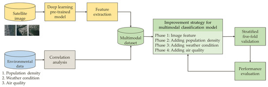
Figure 1.
Study flow chart.
2.3. Approach 1: Multimodal Data Fusion Using Deep Learning
This study compared the classification performance of several common deep learning models for remote sensing satellite images, using the accuracy value (ACC) and the confusion matrix as performance evaluation metrics. The deep learning models used were as follows: EfficientNetV2B2 [18], EfficientNetV2B3 [18], ResNet50 [19], VGG16 [20], and DenseNet169 [21].
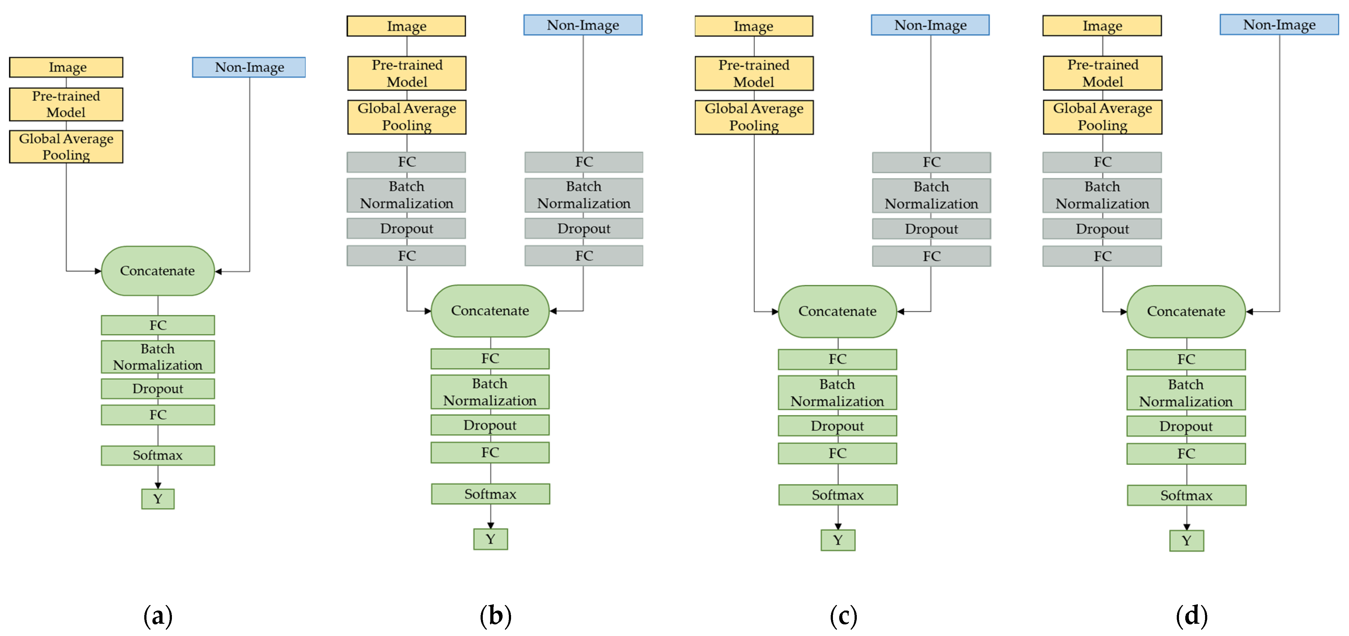
Next, the best-performing deep learning model in image classification was selected as the pre-trained model for images, followed by a global average pooling layer. Fusion was performed using concatenation, a part of the operation-based fusion technique. Four different architectures of multimodal deep learning models were compared, as shown in Figure 2. The first architecture (named MM-DL1) fused the extracted image features directly with environmental data, followed by fully connected layers, a batch normalization layer, and a dropout layer, before predicting using a softmax layer. The second type (named MM-DL2), based on the previous architecture, added fully connected layers, batch normalization layers, and dropout layers separately before fusing image and non-image data. The third architecture (named MM-DL3) only added additional layers for processing non-image data, while the fourth architecture (named MM-DL4) only added them for processing images. The classification performances of the multimodal models were evaluated similarly, by computing the ACC and confusion matrix.
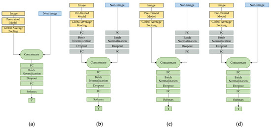
Figure 2.
Multimodal data fusion architectures using a deep learning approach. (a) MM-DL1; (b) MM-DL2; (c) MM-DL3; (d) MM-DL4.
2.4. Approach 2: Multimodal Data Fusion Using Transfer Learning and Machine Learning
The best-performing deep learning model for images in Section 2.3 was selected as the image feature extractor. Transfer learning techniques were used for feature extraction, which involved loading the pre-trained model as the feature extractor, excluding the last classification layer, and adding a global average pooling layer. Through deep learning models, automated feature extraction can be achieved, obtaining higher-level and more abstract feature representations. Each image was passed through the selected deep learning model to obtain its feature representation, which was then used as input for subsequent machine learning tasks. This approach not only accelerates the training process but also enables a wider range of applications.
For machine learning, the features extracted by the selected model were first merged with the previous environmental data to complete the construction of the multimodal dataset. The merged multimodal dataset was standardized to ensure similar ranges between each feature, thereby improving the stability of the model. Subsequently, machine learning models were utilized to predict visibility classification using the multimodal dataset, as shown in Figure 3. A five-fold cross-validation method was employed to improve the generalization ability of the models. Due to the relative maturity of machine learning techniques, various models were compared to identify the best results. The models used were as follows: decision tree, bootstrap aggregation (bagging), random forest, gradient boosting classification tree (GB), extreme gradient boosting classification tree (XGB), histogram-based gradient boosting classification tree (HistGB), K-nearest neighbors (KNN), linear support vector machine (linear SVM), support vector machine with radial basis function kernel (RBF SVM), Gaussian naive Bayes (GaussianNB), logistic regression, and multilayer perceptron (MLP).
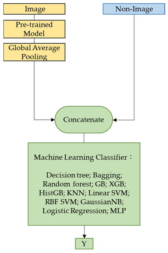
Figure 3.
Multimodal data fusion combining transfer learning and machine learning methods.
To train and test the model, a method of progressively adding features was employed, using the ACC and confusion matrix as performance evaluation metrics. In the prediction of visibility, training began by utilizing the image features extracted by the deep learning model. In the second stage, geographical location data, such as population density, were added. The third stage involved the addition of weather data, such as temperature and precipitation. Finally, in the last stage, air quality data, such as concentrations of various pollutants, were incorporated. We observed the changes before and after adding environmental data, compared the use of different features and the performance differences between each classifier, and then built the best classification model.
3. Experimental Results
This study is a multiclass classification task investigating the impact of different multimodal features and models on visibility classification performance. Section 3.1 presents the results of the correlation analysis. In Section 3.2, the differences in classification performances among several deep learning models for the image are explored. Section 3.3 shows the results of the deep learning multimodal model. Section 3.4 compares the performances of different machine learning models and investigates whether classification performance can be improved by adding different types of features.
3.1. Environmental Data Correlation Analysis
Regarding the environmental data, a correlation analysis was initially conducted to aid in understanding the relationship between various features and visibility. This involved calculating the Pearson correlation coefficient between each feature and the classification labels (visibility).
Table 3 presents the results of the correlation analysis of the environmental data. Among the features, relative humidity shows a relatively high correlation coefficient with visibility, reaching −0.329.
Table 3.
Environmental data correlation analysis results.
3.2. Visibility Classification Using Deep Learning and Satellite Images
This section describes how the classification performances of five common deep learning models were first investigated, implemented using the Tensorflow 2.8 library, with ACC used as the performance evaluation metric. The results are shown in Table 4. Figure 4 shows the test confusion matrix for the best-performing model, with diagonal color marks indicating correctly predicted classes. From Table 4, it can be seen that, when using the VGG16 pre-trained model as the backbone of the classification model, the test ACC is higher, reaching 0.880. Therefore, the VGG16 model was selected as the feature extractor for this study.
Table 4.
Performance evaluation of five deep learning pre-trained models using imagery alone.
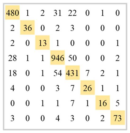
Figure 4.
Test confusion matrix for the best deep learning model using imagery alone.
After selecting the feature extractor, transfer learning techniques were used for feature extraction. This involved loading the VGG16 pre-trained model as the feature extractor, excluding the last classification layer, and adding a global average pooling layer. In total, 512 image features can be extracted for subsequent machine learning tasks.
3.3. Visibility Classification Using Deep Learning and Multimodal Data
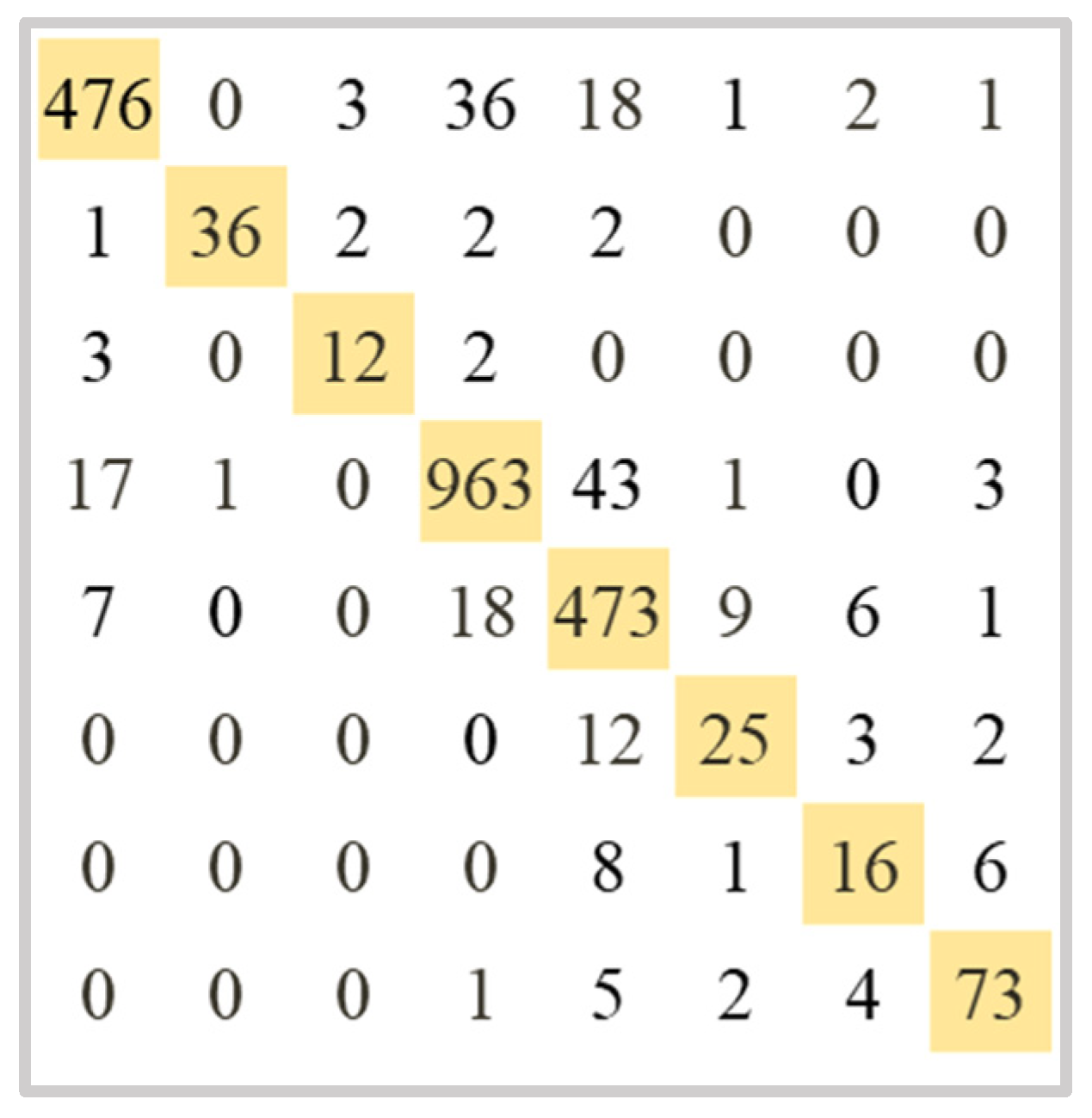
In this section, the classification performances of multimodal deep learning models with four different architectures are discussed, using the ACC and confusion matrix as performance evaluation metrics. All four architectures were trained with the same parameters. The results are shown in Table 5 and Figure 5. We can observe that MM-DL3, which only adds additional layers for processing non-image data, yields the best results, achieving a test ACC of 0.903, while MM-DL4 performs the worst, reaching only 0.854. Figure 5 shows the test confusion matrix for MM-DL3, with diagonal color marks indicating correctly predicted classes.
Table 5.
Performance evaluation of four multimodal deep learning architectures.
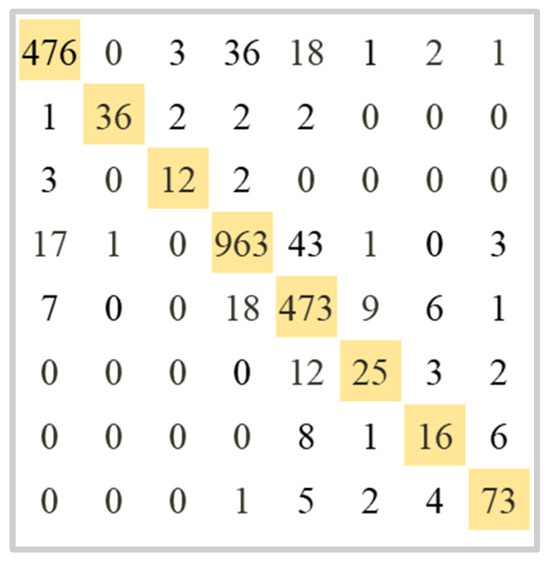
Figure 5.
Test confusion matrix for the best multimodal deep learning model.
3.4. Visibility Classification Using Transfer Learning, Machine Learning, and Multimodal Data
In this section, the impact of different machine learning classification models on classification performance is explored. This is then divided into four phases to sequentially add environmental data and compare the changes before and after. The machine learning models used in this section are all from the Sklearn library, and their parameters are set to the default values of the Sklearn library.
In the second approach, we first trained and tested the models using features extracted from satellite images, employing a five-fold cross-validation method. This study calculates the ACC for both training and testing. Table 6 compares the performance of 12 machine learning models. We observe that, when using only image features, KNN achieves the best classification performance. The test ACC reaches 0.790 ± 0.009, less than the performance of the deep learning models. To further enhance the classification performance, subsequent experiments continued by sequentially adding different aspects of environmental data.
Table 6.
Performance evaluation of 12 machine learning classifiers using image features alone.
Table 7 shows the results when the population density is added as a classification feature. Similarly, the performance of 12 machine learning models is compared. We observe that all classification models show an improvement in performance after the new feature is added. HistGB experiences a significant increase in classification performance, with the test ACC rising from 0.703 ± 0.008 to 0.805 ± 0.006, a 10% increase, becoming the best result for this phase. Conversely, the performance of KNN shows little change, only increasing by 0.004.
Table 7.
Performance evaluation of 12 machine learning classifiers after adding population density.
Table 8 presents the results when weather conditions are further added as classification features, resulting in a total of 523 features. The performance of 12 machine learning models is compared. The XGB classifier achieves the highest test ACC, increasing from 0.802 ± 0.009 to 0.976 ± 0.005, nearly a 20% improvement, surpassing the HistGB classifier to become the best classification model. All the classification models show great improvement in performance, except for the Bayes model, which still performs poorly.
Table 8.
Performance evaluation of 12 machine learning classifiers after adding weather conditions.
Table 9 shows the results when air quality is further added as a classification feature, including the concentrations of various pollutants, resulting in a total of 530 features. The results of different machine learning classifiers are compared. The XGB classifier continues to exhibit the best classification performance, with the test ACC increasing from 0.976 ± 0.005 to 0.978 ± 0.002. Compared to the results when the weather conditions were added, there is limited overall change in classification performance, suggesting that the concentrations of various pollutants may not be the most critical factors affecting visibility.
Table 9.
Performance evaluation of 12 machine learning classifiers after adding air quality.
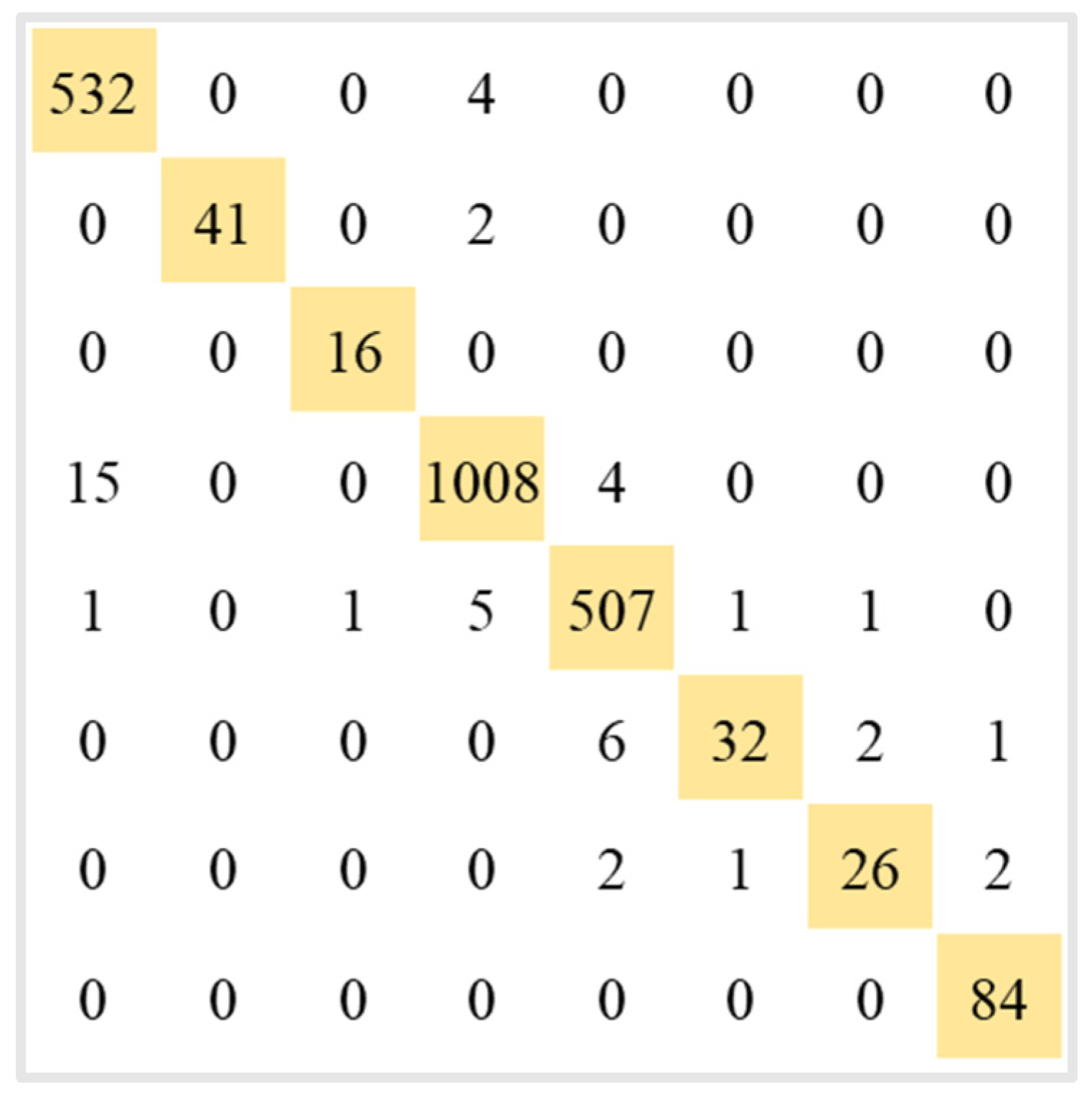
Figure 6 shows the performance differences among various classification models. For the visibility classification task, the XGB classifier achieves the best performance, with a test ACC of 0.978 ± 0.002.The confusion matrix is shown in Figure 7, with diagonal color marks indicating correctly predicted classes. Therefore, for the visibility classification task, VGG16 was selected as the feature extractor, combined with the XGB classifier to establish the optimal model.
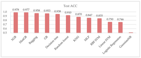
Figure 6.
Performance comparison of 12 machine learning classifiers.
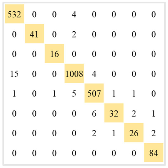
Figure 7.
Test confusion matrix of XGB classifier.
4. Discussion
4.1. Performance Comparison after Adding Environmental Data Features
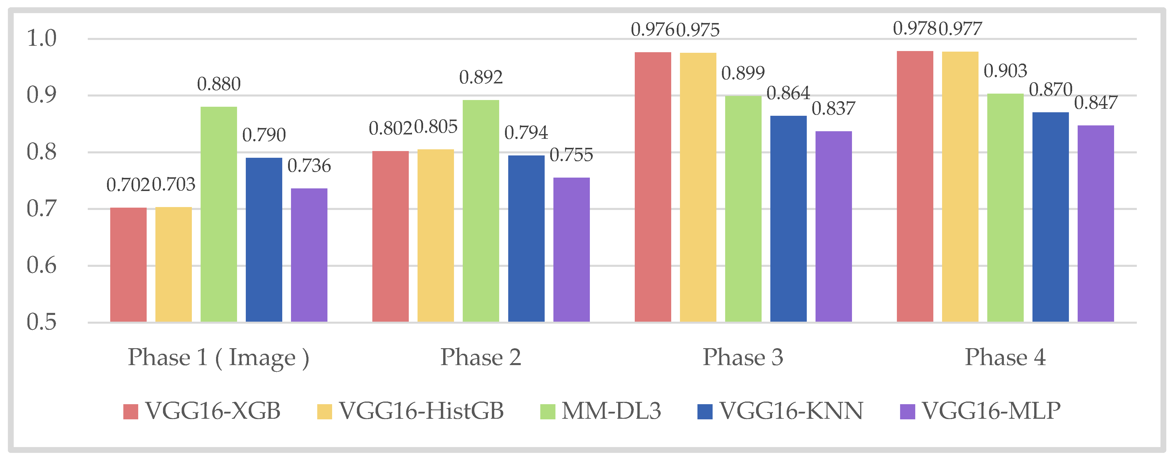
Table 10 compares classification performance in four stages on the basis of results from Section 3.3 and Section 3.4. The best architectures in Section 3.3 and the better four machine learning models selected in Section 3.4 are compared. Note that the parameters for the MLP were set to default values found in the Sklearn library. From Figure 8, it can be observed that the test accuracy values increase steadily. In visibility multiclass classification, the XGB classifier emerges as the best classification model, with a test ACC of 0.978. However, the performance improvement of incorporating air quality data in the final phase is not significant. If considering reducing model complexity in the future, achieving good performance may only require adding weather conditions.
Table 10.
Performance comparison in four stages using different methods.

Figure 8.
Performance comparison in four stages using different models.
Comparing the two approaches, when using multimodal deep learning models for classification, the increase in classification performance is limited. This limitation could be attributed to the model’s constraints; as XGB belongs to ensemble learning techniques, it improves the overall model performance by integrating multiple weak learners, such as decision trees. In contrast, deep learning classification relies solely on a single neural network, rather than multiple learners.
Visibility prediction work can be divided into classification tasks [9,10] and regression tasks [6,11]. We compared the performance of our approach with previous studies on visibility classification. Table 11 provides a comparative summary of these methods according to year, author, method, data type, number of class, data size, and test set accuracy. Since this study focuses on developing visibility classification models, Table 11 uses test set accuracy (Test ACC) for performance evaluation [9,10]. Due to the use of different datasets in various studies, making direct comparisons is challenging. Despite this difference, our proposed method demonstrates excellent performance. Previous studies typically used ground images for their research [6,9,10], whereas our study employs satellite remote sensing images for visibility classification. When compared with existing approaches [9,10] that solely used images for classification, our study demonstrates that incorporating images and environmental tabular data can enhance overall test set accuracy. Furthermore, unlike previous studies that exclusively relied on deep learning methods [6,9,10] or machine learning techniques [11], we combine both deep learning and machine learning approaches to construct our models. As a result, our approach effectively improves visibility classification performance, leading to better outcomes.
Table 11.
Performance comparison with previous studies.
4.2. Limitations and Future Work
This study has three research limitations. First, there is the issue of data imbalance: the visibility dataset exhibits severe imbalance. This is due to the lower number of data points available for visibility classified as less than 6 km and greater than 16 km. Second, there are limitations regarding geographical regions and data coverage duration. This study only utilizes data from the winter season in Taiwan; thus, incorporating data from other regions and seasons would enhance the model’s generalization capability. Lastly, there are constraints related to model development. This study only employs feature extraction methods to process images and uses a simple fusion technique.
To address the issue of data imbalance, future research should collect more diverse data across different seasons and geographical regions, beyond just the winter season in Taiwan. For model development, future research should also explore more multimodal data fusion techniques with different architectures and investigate the ensemble method in deep learning models [22]. Additionally, the authors of this study plan to develop a real-time visibility detection system to provide suggestions for outdoor activities and allow users to monitor environmental safety at any time.
5. Conclusions
This study combines satellite remote sensing images with environmental data to explore two different multimodal data processing methods. Combining transfer learning and machine learning classifiers is the best visibility classification method, which can effectively improve classification performance. Based on the experimental results, the VGG16 pre-trained model was chosen as the image feature extractor. Subsequently, different environmental data features were incrementally added, and the training process was repeated. Ultimately, the XGB classifier was used, resulting in a test accuracy of 0.978 ± 0.002. The inclusion of environmental data led to improvements of 9.8%. In summary, this study first established a multimodal visibility dataset by integrating remote sensing images and environmental monitoring data and successfully established the best visibility classification model using the VGG16 image feature extractor combined with the XGB classifier. In terms of environmental data relationships, weather conditions have a significant impact on visibility, while the concentration of various pollutants may not be the most critical factors affecting visibility.
Author Contributions
Conceptualization, M.-H.T.; methodology, H.-Y.T. and M.-H.T.; software, H.-Y.T. and M.-H.T.; formal analysis, H.-Y.T. and M.-H.T.; writing—original draft preparation, H.-Y.T.; writing—review and editing, M.-H.T.; supervision, M.-H.T. All authors have read and agreed to the published version of the manuscript.
Funding
This research was funded by the National Science and Technology Council, Taiwan, R.O.C., grant number NSTC 112-2121-M-040-001.
Data Availability Statement
Data used in this study are sourced from publicly available websites. Readers who require data and code assistance are asked to contact the corresponding authors.
Conflicts of Interest
The authors declare no conflicts of interest.
References
- Hyslop, N.P. Impaired visibility: The air pollution people see. Atmos. Environ. 2009, 43, 182–195. [Google Scholar] [CrossRef]
- Tsai, Y.I. Atmospheric visibility trends in an urban area in Taiwan 1961–2003. Atmos. Environ. 2005, 39, 5555–5567. [Google Scholar] [CrossRef]
- Zheng, Y.; Liu, F.; Hsieh, H.-P. U-air: When urban air quality inference meets big data. In Proceedings of the 19th ACM SIGKDD International Conference on Knowledge Discovery and Data Mining, Chicago, IL, USA, 11–14 August 2013; pp. 1436–1444. [Google Scholar]
- Chang, C.-C.; Li, Y.-Z.; Wu, H.-C.; Tseng, M.-H. Melanoma detection using XGB classifier combined with feature extraction and K-means SMOTE techniques. Diagnostics 2022, 12, 1747. [Google Scholar] [CrossRef] [PubMed]
- Sayed, A.R.; Khafagy, M.H.; Ali, M.; Mohamed, M.H. Predict student learning styles and suitable assessment methods using click stream. Egypt. Inform. J. 2024, 26, 100469. [Google Scholar] [CrossRef]
- Li, S.; Fu, H.; Lo, W.-L. Meteorological visibility evaluation on webcam weather image using deep learning features. Int. J. Comput. Theory Eng 2017, 9, 455–461. [Google Scholar] [CrossRef]
- Ortega, L.; Otero, L.D.; Otero, C. Application of machine learning algorithms for visibility classification. In Proceedings of the 2019 IEEE International Systems Conference (SysCon), Orlando, FL, USA, 8–11 April 2019; pp. 1–5. [Google Scholar]
- Palvanov, A.; Cho, Y.I. Visnet: Deep convolutional neural networks for forecasting atmospheric visibility. Sensors 2019, 19, 1343. [Google Scholar] [CrossRef] [PubMed]
- Wang, H.; Shen, K.; Yu, P.; Shi, Q.; Ko, H. Multimodal deep fusion network for visibility assessment with a small training dataset. IEEE Access 2020, 8, 217057–217067. [Google Scholar] [CrossRef]
- Liu, Z.; Chen, Y.; Gu, X.; Yeoh, J.K.; Zhang, Q. Visibility classification and influencing-factors analysis of airport: A deep learning approach. Atmos. Environ. 2022, 278, 119085. [Google Scholar] [CrossRef]
- Zhang, C.; Wu, M.; Chen, J.; Chen, K.; Zhang, C.; Xie, C.; Huang, B.; He, Z. Weather visibility prediction based on multimodal fusion. IEEE Access 2019, 7, 74776–74786. [Google Scholar] [CrossRef]
- Holste, G.; Partridge, S.C.; Rahbar, H.; Biswas, D.; Lee, C.I.; Alessio, A.M. End-to-end learning of fused image and non-image features for improved breast cancer classification from mri. In Proceedings of the IEEE/CVF International Conference on Computer Vision, Montreal, BC, Canada, 11–17 October 2021; pp. 3294–3303. [Google Scholar]
- Pan, S.J.; Yang, Q. A survey on transfer learning. IEEE Trans. Knowl. Data Eng. 2009, 22, 1345–1359. [Google Scholar] [CrossRef]
- Hussain, M.; Bird, J.J.; Faria, D.R. A study on cnn transfer learning for image classification. In Advances in Computational Intelligence Systems, Proceedings of the 18th UK Workshop on Computational Intelligence, Nottingham, UK, 5–7 September 2018; Springer: Berlin/Heidelberg, Germany, 2019; pp. 191–202. [Google Scholar]
- Google Maps Platform. Available online: https://developers.google.com/maps/ (accessed on 12 December 2022).
- Department of Household Registration, Ministry of the Interior. Republic of China(Taiwan). Available online: https://www.ris.gov.tw/app/portal/346 (accessed on 12 December 2022).
- BreezoMeter. Available online: https://docs.breezometer.com/ (accessed on 12 December 2022).
- Tan, M.; Le, Q. Efficientnetv2: Smaller models and faster training. In Proceedings of the International Conference on Machine Learning, Online, 18–24 July 2021; pp. 10096–10106. [Google Scholar]
- He, K.; Zhang, X.; Ren, S.; Sun, J. Deep residual learning for image recognition. In Proceedings of the IEEE Conference on Computer Vision and Pattern Recognition, Las Vegas, NV, USA, 27–30 June 2016; pp. 770–778. [Google Scholar]
- Simonyan, K.; Zisserman, A. Very deep convolutional networks for large-scale image recognition. arXiv 2014, arXiv:1409.1556. [Google Scholar]
- Huang, G.; Liu, Z.; Van Der Maaten, L.; Weinberger, K.Q. Densely connected convolutional networks. In Proceedings of the IEEE Conference on Computer Vision and Pattern Recognition, Honolulu, HI, USA, 21–26 July 2017; pp. 4700–4708. [Google Scholar]
- Tseng, M.-H. GA-based weighted ensemble learning for multi-label aerial image classification using convolutional neural networks and vision transformers. Mach. Learn. Sci. Technol. 2023, 4, 045045. [Google Scholar] [CrossRef]


Disclaimer/Publisher’s Note: The statements, opinions and data contained in all publications are solely those of the individual author(s) and contributor(s) and not of MDPI and/or the editor(s). MDPI and/or the editor(s) disclaim responsibility for any injury to people or property resulting from any ideas, methods, instructions or products referred to in the content. |
© 2024 by the authors. Licensee MDPI, Basel, Switzerland. This article is an open access article distributed under the terms and conditions of the Creative Commons Attribution (CC BY) license (https://creativecommons.org/licenses/by/4.0/).