Influence Maximization in Temporal Social Networks with the Mixed K-Shell Method

Abstract

The study of influence maximizing in temporal social networks (IMT) is an important aspect of influence maximization (IM) research. Currently, two main types of algorithms can solve the IMT problem: greedy-based algorithms and heuristic-based algorithms. However, the greedy-based algorithm is too time-consuming to be used in practice, and most existing heuristic methods do not consider the attributes of nodes, resulting in these methods being unable to solve the IMT problem. Therefore, this paper proposes a mixed k-shell (MKS) algorithm, which considers nodes’ local and global attributes to characterize their influence and select seed nodes. At the local level, we consider the degree centrality of nodes, and at the global level, we propose the temporal k-shell decomposition (TKS) algorithm. Ultimately, the influence of a node is determined by combining the influence of itself and its neighbors. Experiments on four real temporal social networks show that MKS performs better in effectiveness than other heuristic baselines and can maintain a balance between effectiveness and efficiency, providing a useful solution for solving the IMT problem.

1. Introduction

Influence maximization (IM) is an important research direction in social network analysis. It models the users and their connections in the network as nodes and edges, with the goal of finding the most influential set of nodes, so that the influence can spread in the widest range within the network starting from that set. IM has essential applications in various fields, such as online advertising [1], viral marketing [2], and rumor control [3]. Unlike traditional social networks, temporal social networks record the specific time points of interactions between nodes. These time points, reflecting the temporal characteristics of node interactions, play a crucial role in temporal social networks. For example, an email network is a typical temporal network where the transmission of emails has temporal characteristics.

Figure 1 displays the distinction between traditional and temporal social networks. In this Figure, the left side is a traditional network, and the right side is a temporal network. The difference between the two sides lies in that the edges between nodes in the temporal network have a set of values representing the time moment of their interaction. For example, the value set {1, 2} on the edge between nodes $a$ and $c$ in the temporal network indicates that these two nodes interact at time points 1 and 2, while not at other times.

Next, we compare the differences between traditional and temporal networks in calculating node influence based on Figure 1. In the traditional social network, node $a$ attempts to activate its neighbor node $c$. Assuming node $c$ is successfully activated, it will then try to activate its neighboring nodes $d$ and $e$. If only $d$ is activated, it will attempt to activate its neighbor $b$. If $b$ is successfully activated, the influence of $a$ is the number of activated nodes, which is 3. However, in the temporal social network, it is assumed that $a$ activates $c$ at time 1 and activates $d$ at time 3. However, when $d$ attempts to activate $b$, due to no contact between $d$ and $b$ after time 2, $d$ cannot activate $b$. Therefore, the influence of $a$ is 2 in the temporal social network.

From the above example, it can be seen that traditional influence calculation methods are not suitable in temporal networks. Wu et al. [4] were the first to propose the IMT problem. The goal is to find the optimal seeds to maximize influence in a temporal social network. Since the IMT problem is NP-hard, there are two main solutions: one is based on greedy strategies, while the other utilizes heuristic strategies. Greedy strategy-based methods are unsuitable in practice due to the time-consuming Monte Carlo simulations required to estimate node influence. More precisely, the Greedy algorithm starts with an empty seed set, simulates the diffusion process of the seed set, and repeatedly adds an element that gives the maximum marginal gain to the seed set. Since the number of simulation times is usually set to 1000 or 10,000 for each targeted set, the process is very time-consuming. For example, Chen et al. [5] reported that on a directed graph with 76 K nodes and 509 K edges, it took 62 h to find 50 seeds. Heuristic strategies typically rank the influence of nodes and select the top-ranked nodes as seeds. There are two most commonly used heuristic methods: one is based on local centralities, such as degree centrality [6] and PageRank centrality [7], and the other is based on global centralities, such as betweenness centrality [8] and closeness centrality [9], k-shell [10], etc. Among them, methods such as betweenness centrality and closeness centrality, which require information about the entire network structure, are very time-consuming in large-scale networks and cannot be applied in practice.

The global-based k-shell or k-core decomposition method is often used to find influential nodes. The main drawback of this method is that it assumes that nodes within the same core have the same impact, which is unrealistic. To address this issue, Zhu et al. [11] proposed two improved k-shell decomposition methods, called KT and KTIM, which utilize the temporal core information to solve the IMT problem. However, decomposing solely based on temporal cores is insufficient and may not be appropriate in some cases. Therefore, to solve the IMT problem, we propose a mixed k-shell (MKS) algorithm that utilizes both the local and global attributes of nodes. Overall, our main contributions are as follows:

• We propose the MKS algorithm by considering both the local and global attributes of nodes. For local attributes, we evaluate the nodes’ influence based on degree centrality. For global attributes, we present a temporal k-shell decomposition (TKS) algorithm to layer the network onto a different temporal k-shell. Then, we estimate the global influence of nodes based on the temporal k-shell and classic k-shell methods.
• The proposed MKS algorithm only uses the inherent information of the network and does not need any free parameters or human experience, saving the time needed to adjust optimal parameters.
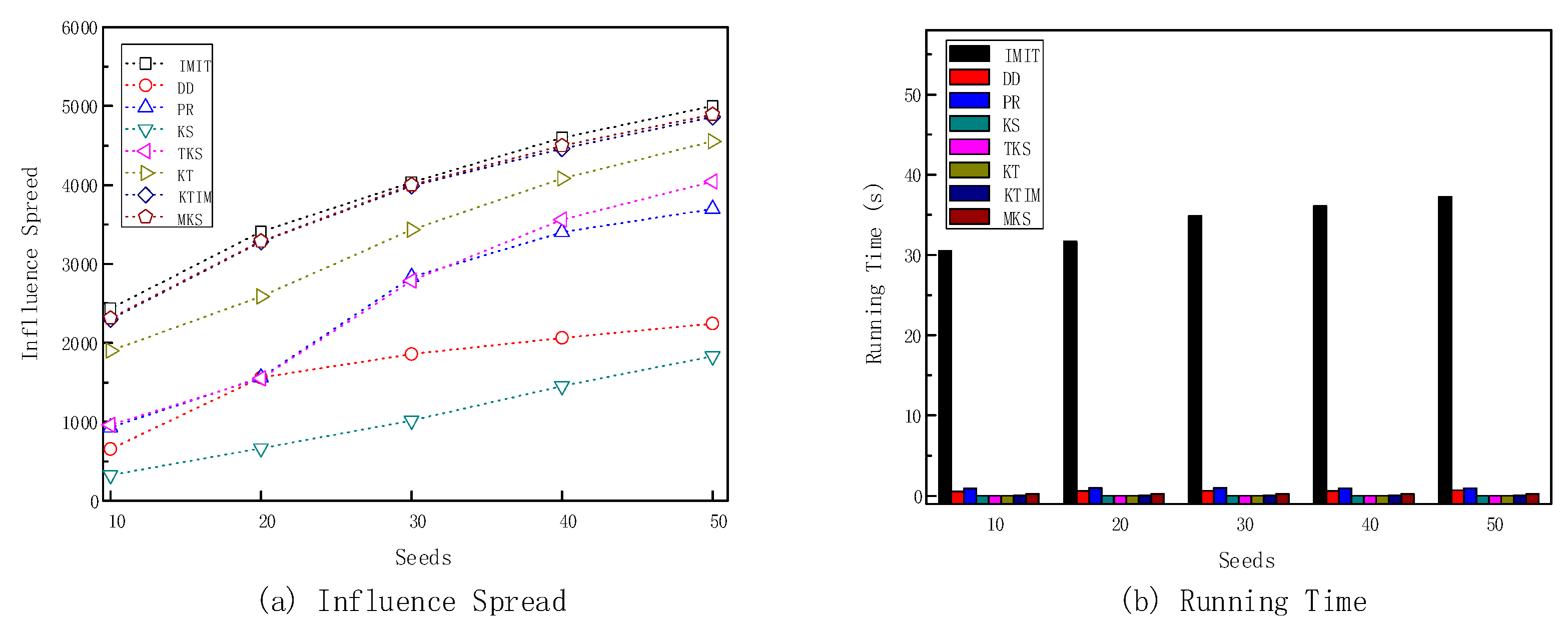
• We carry out experiments on four real-world temporal datasets. The results show that MKS performs more effectively than other heuristic baselines. The ablation study further demonstrates the effectiveness of MKS in considering the local and global attributes of nodes.

We organize the rest of the paper as follows: Section 2 introduces the related work, and preliminaries are discussed in Section 3, followed by methodology in Section 4. Experiments are conducted and analyzed in Section 5, and the paper concludes in Section 6.

2. Related Work

Domingos et al. [12] used Markov random fields to simulate individual behavior, laying the foundation for research on maximizing social influence. Subsequently, Kempe et al. [13] first proposed IM and expanded the research field by introducing the independent cascade (IC) and the linear threshold (LT) influence diffusion models. These models simulate the process of nodes receiving and transmitting information in the network, becoming essential tools for analyzing IM problems.

To solve the IM problem, Kempe et al. [13] first proposed a greedy-based simulation algorithm, which can achieve a (1 − 1/e) approximation guarantee. However, this algorithm is too time-consuming to use in large-scale networks. Leskovec et al. [14] further proposed the CELF algorithm by utilizing the submodularity and monotonicity of the influence propagation function. Subsequently, Goyal et al. [15] optimized CELF and proposed CELF++ to improve efficiency further. In addition, Borgs et al. [16] proposed the RIS method, which selects the nodes that cover the most reverse reachable sets as seeds. Later, Tang et al. [17,18] improved RIS and presented relatively efficient TIM and IMM algorithms. While these algorithms have seen enhanced performance, the time complexity remains challenging when dealing with large-scale networks.

Therefore, many studies have turned to exploring heuristic algorithms. Chen et al. [19] proposed the PMIA algorithm, which simulates influence diffusion based on the local tree structure. This transformation significantly improves the speed of influence calculation. Further, Jung et al. [20] proposed the IRIE algorithm, which combines global influence ranking and local estimation to improve the efficiency of seed selection. Chen et al. [21] proposed the DegreeDiscount algorithm to select seeds by considering the degree of the nodes and their neighbors. In addition, some studies have proposed voting-based algorithms to identify influential nodes, e.g., self-voting [22] and adaptive-voting [23]. Additionally, there are many studies on the extended applications of IM, such as those based on target [24], location [25], community [26], etc.

Recently, researchers have started to consider the IMT problem based on the fundamental IM problem. For example, Li et al. [27] proposed a greedy-based algorithm utilizing the latency-aware independent cascade model to capture the dynamic characteristics of temporal social networks. Wu et al. [4] abstracted the temporal social network as a temporal graph and proposed the independent cascade on temporal graph (ICT) model. They proposed the IMIT algorithm through Monte Carlo simulation and CELF optimization. Later, Chen et al. [28] proposed the TIM algorithm consisting of time-heuristic and time-greedy stages. This algorithm selects candidate nodes based on node attributes in the time-heuristic phase, and then optimizes the nodes’ marginal gain to select seed nodes in the time-greedy phase. Although TIM has improved efficiency, its long operation time in the time-greedy phase is still a limiting factor. Wang et al. [29] proposed an algorithm combining greedy and heuristic strategies to maximize influence in temporal social networks. To improve efficiency, the latest studies have focused on heuristic strategies to solve the IMT problem [30,31].

There are also some heuristic strategies that have been designed by integrating node attributes. For instance, Salavati et al. [32] considered community partitioning and proposed a new centrality metric based on the local structure of nodes, called Gateway Local Rank (GLR). However, this method did not take into account the temporal dynamics of the network, which limited its effectiveness in temporal social networks. Michalski et al. [33] introduced an entropy-based method to examine how a node’s neighborhood changes over time and select potential seeds. Although this method conducted a thorough analysis at the local level, it did not consider the global perspective. Additionally, Zhu et al. [11] utilized node attributes to solve the TIM problem. However, their methods only considered temporal cores and included a free parameter called candidate seed size, which meant that their method is not robust to the structure of the network. As far as we know, our work is the first to consider both cores and temporal cores and use the local and global attributes of nodes to solve the IMT problem.

Besides the issue of IMT, there are many other related studies in temporal networks. For example, Zhang et al. [34] proposed an IM framework based on prediction and replacement using machine learning technology. By analyzing historical network snapshots, they can predict future network states and identify seed nodes suitable for dynamic networks. Chandran et al. [35] proposed a seed selection method utilizing dynamic influence. They introduced a two-hop triangle influence to estimate the node’s influence.

3. Preliminaries

In this section, we first introduce the temporal social network and the influence diffusion model. Then, we propose the formal definition of IMT and the classic k-shell algorithm. We also discuss the drawbacks of the k-shell algorithm.

3.1. Temporal Social Network and Influence Diffusion Model

The temporal social network is a way of modeling social structure over time. It can be modeled as $G_T=(V,E,T_E$), where $V$ stands for the set of nodes, $E$ represents the set of edges, where each edge is a tuple $\left(u,v\right)$, denoting a connection from node $u$ to node $v$, and $T_E$ indicates the set of times at which interactions occur between pairs of nodes.

Figure 2 shows a toy temporal social network with 12 nodes and 16 edges. It is observed that nodes can only interact at a specific time, e.g., $T_{\left(g,h\right)}=\left\{1, 2\right\}$ means that nodes $g$ and $h$ only interact at times 1 and 2. $T_{\left(g,e\right)}=\left\{3\right\}$ indicates an interaction between nodes $g$ and $e$ at time 3. It is easy to see that instead of seeing a network as a static snapshot, temporal social networks can capture the features of the formation, activation, and dissolution of connections over time.

The IC model [13] is a widely used influence diffusion model in IM. However, it cannot be directly used in temporal social networks as it does not consider the interaction times of nodes. Wu et al. [4] expanded the IC model to the ICT model to mimic the spread of influence within temporal social networks. This paper also uses the ICT model to simulate the diffusion of nodes’ influence. Given a temporal social network $G_T=(V,E,T_E$), let the active start time of each node $v\in V$ be marked as $Ac{t}_v=-1$, indicating that every node is in an inactive state. After selecting a seed node $u$, the influence diffusion process is as below:

(1)

Set the active start time of $u$ to 0, i.e., $Ac{t}_u=0$. At this time, the seed node $u$ has an activation probability $p_{u,v}$ to activate its inactive neighbor node $v$, and $u$ has only one opportunity to activate $v$.

(2)

When $u$ tries to activate $v$, the model first determines whether $Ac{t}_u$ is less than or equal to $\max \left(T_{\left(u, v\right)}\right)$. If it is satisfied, then $u$ will activate $v$ with $p_{u,v}$. Otherwise, $u$ will skip $v$ and try to activate the next inactive neighbor node.

(3)

Whether or not $u$ can activate $v$, in subsequent rounds, $u$ will not try to activate $v$ again.

(4)

Once $v$ is successfully activated, record its active start time $Ac{t}_v=t\left(u,v\right)$, where $t\left(u,v\right)\in T_E$, and $Ac{t}_u\ll t\left(u,v\right)\ll \max \left(T_{\left(u, v\right)}\right)$.

(5)

The influence tries to spread from the newly active nodes to the inactive neighbor nodes in the entire network until no new nodes are activated.

In traditional IM problems, $p_{u,v}$ is usually set to $1/D_v$, where $D_v$ is the degree of $v$. However, in temporal networks, this approach does not take into account interaction times between nodes. For example, consider nodes $k$ and $l$ in Figure 2. Although both nodes have a degree of 1, node $l$ has two interactions, making its likelihood of activation greater than that of node $k$. Therefore, in the ICT model, we use the activation probability proposed in [28], which is represented in Equation (1):

$$p_{u,v}=\frac{\left|T_{u,v}\right|}{{{\displaystyle \sum }}_{w\in N\left(v\right)}\left|T_{w,v}\right|}$$

(1)

where $\left|T_{u,v}\right|$ is the interaction times between nodes $u$ and $v$ and $N\left(v\right)$ is the neighbor set of $v$.

3.2. Influence Maximization of Temporal Social Networks

Wu et al. [4] were the first to propose the IMT problem. Given a temporal social network $G_T=(V,E,T_E$) and an influence diffusion model, such as ICT, the goal of IMT is to find the optimal set of seeds $S$ of size $k$. Under the given influence diffusion model, the influence spread of $S$, $\sigma \left(S\right)$, is maximized. It can be formulated in Equation (2):

$$S^{*}=\underset{S\subseteq V,\left|S\right| = k}{\mathrm{argmax}} \sigma \left(S\right)$$

(2)

A simple way to address this issue is with a greedy algorithm utilizing Monte Carlo simulations. The pseudocode of the algorithm is shown in Algorithm 1:

Algorithm 1: Greedy

Input: $G_T=\left(V,E,T_E\right)$, k Output: $S$ 1:  Let $S=\varnothing$; 2:  for$i=1$ to$k$ do 3:     $u=argma{x}_{u\in V\backslash S}\left\{\sigma \left(S{{\displaystyle \cup }}^{ }\left\{u\right\}\right)-\sigma \left(S\right)\right\}$; 4:     $S=S{{\displaystyle \cup }}^{ }\left\{u\right\}$; 5:  end for 6:  return $S$;

The algorithm starts by initializing an empty seed set $S$ (line 1). Then, it iterates k times (lines 2–5) to find $k$ seeds. In each iteration, it goes through each node in the social network, calculating the gain in influence spread that would result from adding it to the seed set, as estimated by Monte Carlo simulations (lines 3–4). Finally, the obtained seed set is returned (line 6). For time complexity, the iteration runs $k$ times. In each iteration, the simulation runs $O\left(nmr\right)$, where $n$, $m$, $r$ are the number of nodes, number of edges, and number of simulations, respectively. Therefore, Algorithm 1 takes $O\left(knmr\right)$, which is too time-consuming to use in large-scale networks. Thus, we will propose a more efficient algorithm in the next section.

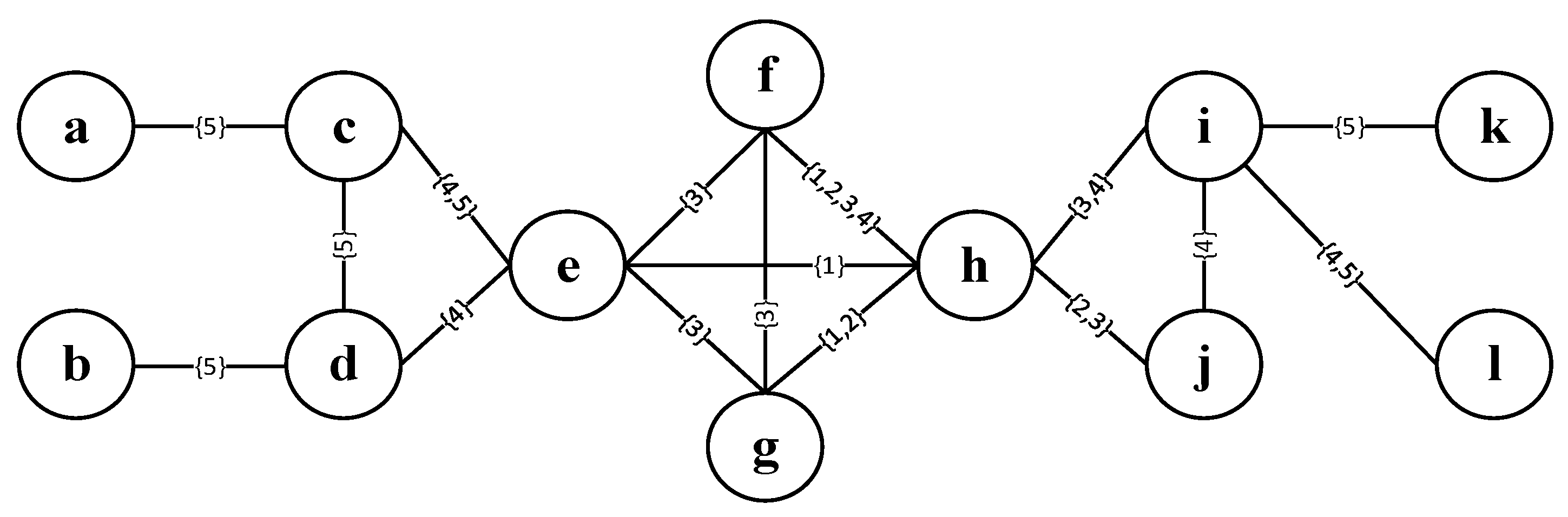
3.3. The K-Shell Decomposition Algorithm

The k-shell algorithm is a famous network decomposition method used in complex network analysis [10]. The main idea behind k-shell decomposition is to categorize nodes based on their degree. We provide the pseudocode of this in Algorithm 2.

Algorithm 2: KS

Input:$G_T=\left(V,E,T_E\right)$ Output:$ks$ 1:  initialize $k=1, ks=\left\{\right\}$ 2:  while$V\ne \varnothing$ 3:  find the set of nodes$S$with a degree no more than k 4:  while $S$ is not empty 5:    for each node $v$ in $S$ 6:       $ks\left[v\right]=k$ 7:    end for 8:    remove all nodes in $S$ and their associated edges from $G_T$ 9:    recalculate the degree of nodes and $S$ from the updated $G_T$ 10:  end while  11:$\hspace{1em} k+=1$ 12:  end while  13:  return$ks$

The algorithm begins with unassigned nodes and iteratively removes fewer degree nodes, starting with $k=1$ (line 1) and incrementing by one each round (line 11). The nodes with degrees equal to or less than $k$ are assigned to the respective k-shell layer and removed from the network, along with their edges (lines 3–10). This process continues until all nodes are assigned a shell. Nodes in higher k-shells are considered more influential within the network, making the method useful for identifying influential nodes.

Figure 3 shows the k-shell decomposition results of the toy network in Figure 2. First, we iteratively find all nodes with degree 1: $a, b, k, l$, and then we delete these nodes and the corresponding edges, assigning them to shell layer 1, i.e., $KS=$1. Next, we identify all nodes with degree 2: $c,d,i,j$, and assign them to shell layer 2, i.e., $KS=$ 2. Finally, we select all nodes with degree 3: $e,f,g,h$, and assign them to shell layer 3, i.e., $KS=$3.

The k-shell method is a technique to characterize the global information of nodes, but a major drawback of k-shell is that it cannot distinguish the influence of nodes within the same shell. Additionally, in temporal networks, the k-shell method does not consider the number of interactions between nodes, so it is not applicable in certain situations. We will elaborate on this in the following section.

4. Methods

In this section, we first provide details of the temporal k-shell decomposition algorithm. Then, by combining the local and global attributes of nodes, we introduce the MKS algorithm.

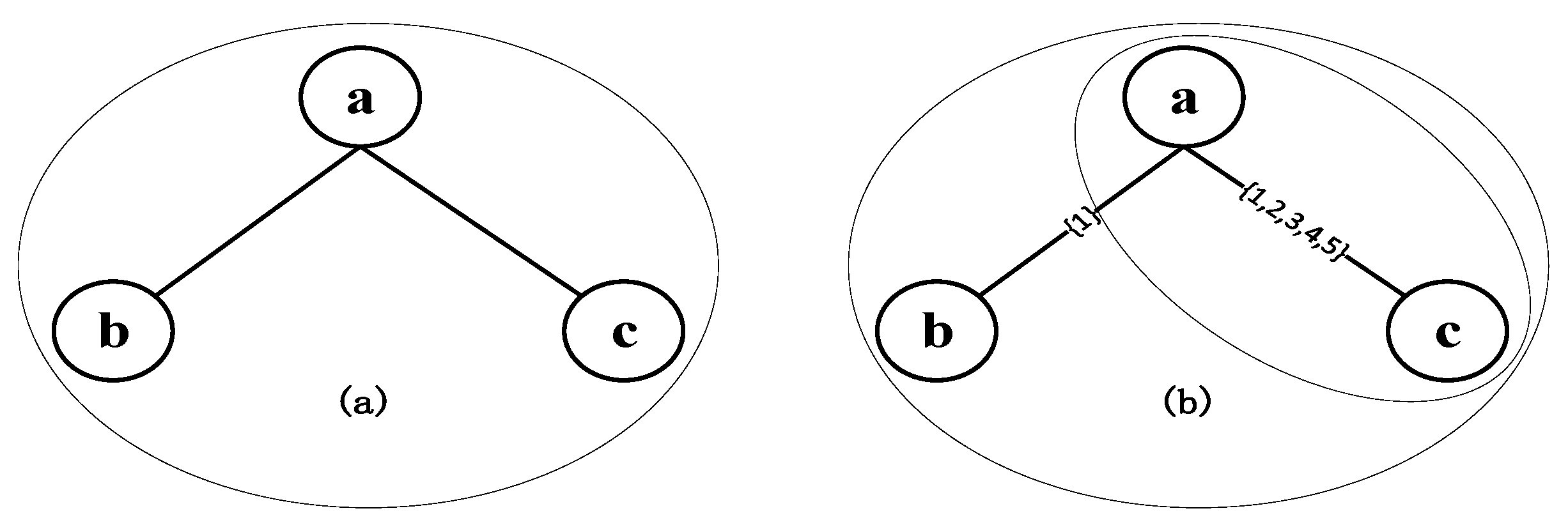
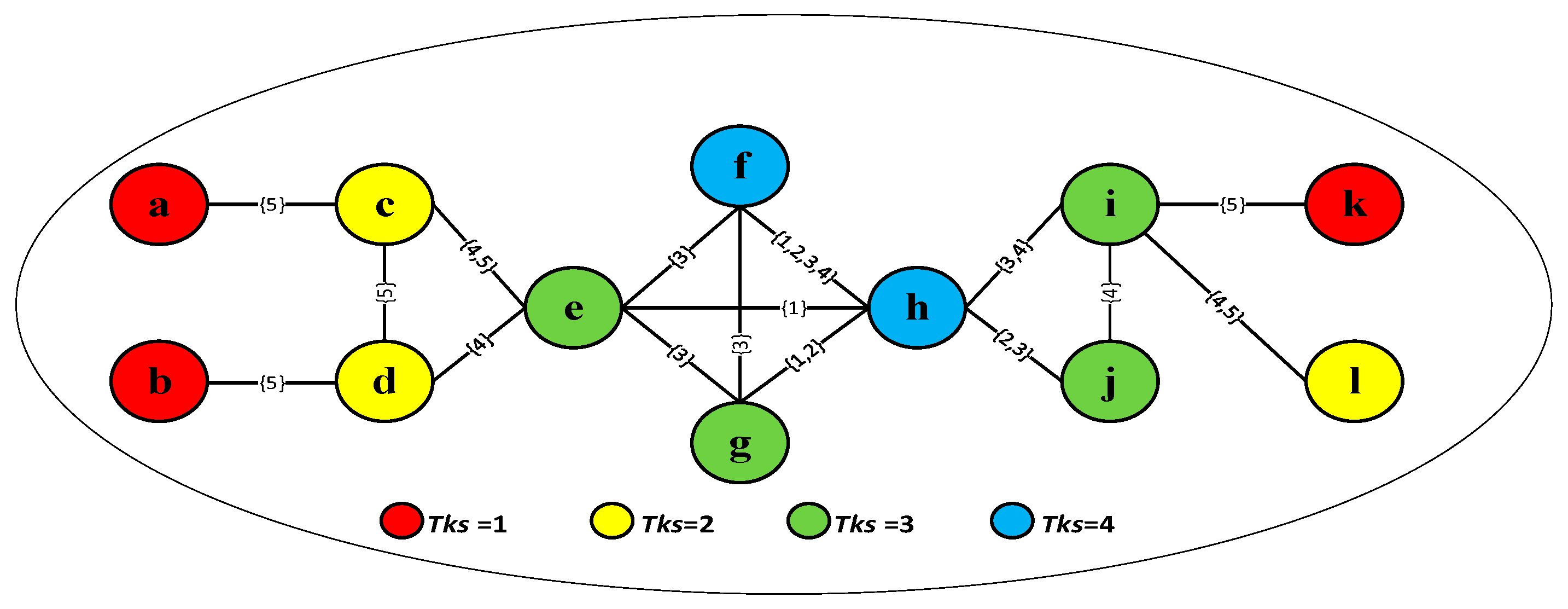
4.1. The Temporal K-Shell Decomposition Algorithm

Because the classical k-shell method does not account for interactions between nodes, it may not accurately reflect the structure of temporal networks where the interactions can be crucial for understanding the nodes’ behavior. Consider the example in Figure 4. Figure 4a is a traditional network without considering node interactions, and Figure 4b is a temporal social network, where nodes $a$ and $b$ interact one time and nodes $a$ and $c$ interact five times. If we do not consider the interactions of nodes, nodes $a$, $b$, and $c$ should be assigned the same shell based on the k-shell algorithm, as shown in Figure 4a. In contrast, since there are more interactions between $a$ and $c$ than between $a$ and $b$, the core levels of $a$ and $c$ should be higher than $b$, as shown in Figure 4b.

On this basis, we propose the TKS algorithm. The core of the algorithm follows a similar iterative process as traditional k-shell decomposition, but instead of using static degrees, it utilizes the interaction times of nodes. Nodes are removed along with their edges if their interaction times fall below the current minimum value. After each removal, the interaction times of the remaining nodes are recalculated to reflect the most current structure of the network. The pseudocode is as follows (Algorithm 3):

Algorithm 3: TKS

Input:$G_T=\left(V,E,T_E\right)$ Output:$tks$ 1:  initialize $tk=1,tks=\left\{\right\}$ 2:  $\mathrm{calculate} \mathrm{the} \mathrm{interaction} \mathrm{times} C_{i }$$\mathrm{for} \mathrm{each} \mathrm{node} i \mathrm{in} G_T$ 3:  $\mathrm{calculate} \mathrm{the} \mathrm{minimum} \mathrm{interaction} \mathrm{times} C_{min}=\min (C_{i }$) 4:  while$V\ne \varnothing$  5:   $\mathrm{find} \mathrm{the} \mathrm{set} \mathrm{of} \mathrm{nodes} S \mathrm{with} \mathrm{interaction} \mathrm{times} \mathrm{no} \mathrm{more} \mathrm{than} C_{min}$ 6:    while $S$ is not empty 7:     for each node $v$ in $S$ 8:       $tks\left[v\right]=tk$ 9:      end for 10:     remove all nodes in $S$ and their associated edges from $G_T$ 11:     recalculate$C_{i }$ and $S$ from the updated $G_T$ 12:   end while  13:   recalculate$C_{i }$$, C_{min}$ 14:   $tk +=1$ 15:  end while  16:  $\mathrm{return} tks$

The algorithm begins with initializing the temporal k-shell index $tk$ to 1 and the temporal k-shell dictionary $tks$ to store the final temporal k-shell values for each node (line 1). Then, it calculates the interaction times $C_{i }$ of each node and their minimum value $C_{min}$ (lines 2–3). The temporal network $G_T$is processed iteratively (lines 4–15). In each iteration, the algorithm removes all nodes with interaction times less than $C_{min}$ and updates the $tks$ dictionary to assign them the current temporal k-shell index (lines 5–12). After each cycle of node removal and dictionary updates, the interaction times $C_{i }$ of each remaining node $i$and the minimum value $C_{min}$ are recalculated to reflect the changes in the network structure caused by the removals (line 13). This process repeats, incrementing $tk$ until no nodes remain. We should note that the proposed TKS algorithm is different from the classical backtracking method in terms of the following perspectives. From the processing perspective, TKS layers nodes by iteratively removing nodes with lower interaction times, whereas backtracking incrementally constructs a solution through try and check. From the application perspective, TKS is a specific network layering technique primarily applied in layering the network, while backtracking is used in a wide range of combinatorial optimization and decision problems.

Figure 5 shows the temporal k-shell decomposition result of the toy network in Figure 2. First, we calculate$C_{min}$ = 1 and find all nodes with interaction times no more than $C_{min}$: $a, b, k$, and then we delete these nodes and associated edges and assign them to temporal shell layer 1. Next, we recalculate $C_{min}$ = 2 and obtain nodes $d$ and $l$ with interaction times no more than $C_{min}$. We assign $d$ and $l$ to temporal shell layer 2 and remove these nodes and their associated edges. Next, we iteratively find another node $c$ with interaction times no more than $C_{min}$. We add it to temporal shell layer 2. Then, we recalculate $C_{min}$ = 3 and obtain nodes $e,i,j,$ and $g$ in temporal shell layer 3. Finally, we calculate and obtain nodes $f$ and $h$ in temporal shell layer 4.

4.2. The Mixed K-Shell Algorithm

The main drawback of KS and TKS algorithms is that they cannot effectively differentiate the influence of nodes in the same layer. Therefore, we propose a heuristic method based on the mixed k-shell algorithm, which considers global and local information and does not assign the same weight to nodes as the traditional k-shell method. We use degree centrality as a local attribute of a node, and k-shell and temporal k-shell as global attributes of a node. This obtains the final influence of a node through its interaction with its neighboring nodes. Our method uses only intrinsic parameters in the network and does not introduce other hyperparameters.

For local attributes, the influence of a node is related to the degree centrality of its neighboring nodes, and the local influence of node i can be defined in Equation (3):

$$In{f}_i^l={\displaystyle {\sum }_{j\in N(i)}{W}_{i,j}^l}$$

(3)

where $N\left(i\right)$ is the neighbor set of node i, $W_{i,j}^l$ is the local influence weight of node $i$ on its neighboring node $j$, as defined in Equation (4), whose value is related to the degree of nodes $i$ and $j$, $d_i$ is the degree of node $i$, $d_j$ is the degree of node $j$, and $d_{\max }$ and $d_{\min }$ are the maximum and minimum degrees of the temporal network, respectively. The goal of min-max normalization is to ensure that the nodes’ weights are within the same range.

$$W_{i,j}^l=\left(d_i-d_{\min }\right)/\left(d_{\max }-d_{\min }\right)+\left(d_j-d_{\min }\right)/\left(d_{\max }-d_{\min }\right)$$

(4)

For global attributes, we first calculate the influence weight $W_{i,j}^{ks}$ of $i$ on its neighbor $j$ in the k-shell structure using Equation (5), and the influence weight $W_{i,j}^{tks}$ of $i$ on its neighbor $j$ in the temporal k-shell structure using Equation (6).

$$W_{i,j}^{ks}=\left(k{s}_i-k{s}_{\min }\right)/\left(k{s}_{\max }-k{s}_{\min }\right)+\left(k{s}_j-k{s}_{\min }\right)/\left(k{s}_{\max }-k{s}_{\min }\right)$$

(5)

$$W_{i,j}^{tks}=\left(tk{s}_i-tk{s}_{\min }\right)/\left(tk{s}_{\max }-tk{s}_{\min }\right)+\left(tk{s}_j-tk{s}_{\min }\right)/\left(tk{s}_{\max }-tk{s}_{\min }\right)$$

(6)

where, $k{s}_i$ and $tk{s}_i$ are the k-shell value and temporal k-shell value of $i$, $k{s}_j$ and $tk{s}_j$ are the k-shell value and temporal k-shell value of $j$,$k{s}_{\max }$ and $k{s}_{\min }$ are the maximum and minimum k-shell values of the temporal network, and$tk{s}_{\max }$ and $tk{s}_{\min }$ are the maximum and minimum temporal k-shell values, respectively.

On this basis, the global influence weight of a node $i$ on node $j$, denoted as $W_{i,j}^g$, is defined in Equation (7):

$$W_{i,j}^g={\lambda }_1\ast W_{i,j}^{k\mathrm{s}}+{\lambda }_2\ast W_{i,j}^{tks}$$

(7)

Here, ${\lambda }_1$ denotes the quotient of the average degree to the average k-shell in the network and ${\lambda }_2$ denotes the quotient of the average degree to the average temporal k-shell in the network. Their value can be obtained by Equation (8):

$$\{\begin{array}{l}k{s}_{avg}={\displaystyle {\sum }_{i=1}^{n}k{s}_i}/n\\ tk{s}_{avg}={\displaystyle {\sum }_{i=1}^{n}tk{s}_i}/n\\ d_{avg}={\displaystyle {\sum }_{i=1}^n{d}_i}/n\\ {\lambda }_1=d_{avg}/k{s}_{avg}\\ {\lambda }_2=d_{avg}/tk{s}_{avg}\end{array}$$

(8)

where, $n$ is the number of nodes, $k{s}_{avg}$ is the average k-shell value of nodes, $tk{s}_{avg}$ is the average temporal k-shell value of nodes, and $d_{avg}$ is the average degree of nodes.

Then, the global influence of node i can be defined as Equation (9):

$$In{f}_i^g={\displaystyle {\sum }_{j\in N(i)}{W}_{i,j}^g}$$

(9)

Finally, according to Equations (3) and (9), the influence of node i is obtained as Equation (10):

$$In{f}_i=In{f}_i^l+In{f}_i^g$$

(10)

Based on the above analysis, we propose the MKS algorithm. The pseudocode is shown in Algorithm 4. The algorithm first calculates the k-shell and temporal k-shell values of nodes based on Algorithms 2 and 3, respectively (lines 1–2). Then, it calculates ${\lambda }_1$,${\lambda }_2$ based on Equation (8) without using any free parameters (line 3). For each node $i$ in the network, it calculates the local and global influence of node $i$ according to the values of degree, k-shell, and temporal k-shell (lines 4–6). Finally, it selects the top $k$ nodes with the largest influence as seeds (lines 7–11).

Algorithm 4: MKS

Input:$G_T=\left(V,E,T_E\right)$, k Output:$S$ 1:  calculate $ks$ according to Algorithm 2 2:  calculate $tks$ according to Algorithm 3 3:  calculate ${\lambda }_1$,${\lambda }_2$ based on Equation (8) 4:  for each node$i \mathrm{in} V$ 5:   calculate$In{f}_i$ according to Equations (3), (9), and (10) 6:  end for 7:  for$j =1 \mathrm{to} k$ 8:   $u=argmax\left\{In{f}_i\right| i ϵ V\backslash S\}$ 9:   $S=S{{\displaystyle \cup }}^{ }u$ 10: end for 11: return $S$

For time complexity, let $\left|V\right|=n$,$\left|E\right|=m$, and $\left|T_E\right|=T$. Line 1 takes $O\left(n*\left(n+m\right)\right)$and line 2 takes $O\left(n*\left(n+T\right)\right).$In the worst case scenario, line 3 takes $O(n$), lines 4–6 take $O(kn{n}_c$), where $n_c$ is the average number of neighbors of nodes in the network, and lines 7–9 take $O(n$). Therefore, the overall time complexity of MKS is $O\left(n*\left(n+T+k{n}_c\right)\right)$. Further, we compare the time complexity of the MKS algorithm with the Greedy algorithm. Since the complexity of Greedy is $O\left(knmr\right)$, where m is the number of edges in the networks, it is commonly larger than node numbers $n$. Therefore, the time complexity of Greedy is larger than $O\left(kr{n}^2\right)$. In addition, $r$ is the simulation time, which is set to 1000 or 10,000. Thus, the time complexity of Greedy is much larger than MKS.

5. Experiments

5.1. Datasets

Four real-world temporal social networks were used in the experiments, including Bitcoin-OTC [36], CollegeMsg [37], Math-Overflow [37] and Ask-Ubuntu [38]. All datasets can be downloaded from http://snap.stanford.edu/data/ (accessed on 10 March 2024). Bitcoin-OTC is a network in which people trade using Bitcoin. CollegeMsg is a temporal network consisting of private messages at the university. Ask-Ubuntu and Math-Overflow are two websites with temporal interactions. An edge $\left(u, v, t\right)$ in these datasets means user $u$ interact with user $v$ at time $t$. The details are shown in

Table 1. The details of datasets.

Datasets	Nodes	Edges	Temporal Edges
Bitcoin-OTC	5881	35,592	35,592
CollegeMsg	1899	20,269	59,835
Math-Overflow	13,840	81,121	195,330
Ask-Ubuntu	75,555	178,210	356,822

.

5.2. Baseline Algorithms

We conducted experimental comparisons between the proposed MKS algorithm and the following baseline algorithms to test their effectiveness and efficiency.

• IMIT [4]. This is a greedy-based simulation algorithm that uses the CELF method to improve efficiency.
• DD [21]. This is a degree-based heuristic algorithm. The basic idea of it is to discount the degree of a node based on the number of neighbors it has in common with already selected seeds.
• PR [7]. This is the classical PageRank algorithm based on the assumption that websites with higher influence are likely to receive more links from other websites.
• KS. Algorithm 2 in our paper. We selected the top $k$nodes with the highest k-shell values as seeds.
• TKS. Algorithm 3 in our paper. We selected the top $k$ nodes with the highest temporal k-shell values as seeds.
• KT [11]. This is a heuristic algorithm that selects the seeds with the largest comprehensive degree in each shell layer.
• KTIM [11]. This is an improved version of KT, which selects the seeds with the largest comprehensive degree within the candidate seed set.

5.3. Experimental Setting

In experiments, we evaluated two metrics: effectiveness and efficiency. Effectiveness refers to comparing the range of the influence spread by the seeds selected from different baseline algorithms under the ICT model. Efficiency is measured by the running time of baselines to select the same number of seeds. In our experiments, we chose 10 to 50 seeds with a step size of 10. The number of Monte Carlo simulations in ICT is set to 1000. For the IMIT algorithm, we obtained the influence spread of each node offline. Otherwise, the running time of the algorithm would be much longer in large-scale networks. For other algorithms, we used the parameters proposed in the original papers. Since the network structure is fixed for the shell-based algorithms, we also obtained the core decomposition results offline. The experiments were conducted in a Windows environment, with an Intel(R) Core(TM) i7-10875H CPU, 16 GB RAM, and a 512 GB hard disk (Lenovo, Beijing, China). All codes were implemented using PyCharm+Python 3.8.

5.4. Main Results

We first evaluated the effectiveness and efficiency of different algorithms. The results are shown in Figure 6, Figure 7, Figure 8 and Figure 9. The seed set size ranges from 10 to 50. To fairly compare the performance of baselines, a consistent test method is adopted in this section: once the algorithm selected a set of seeds, we recorded the running time, then ran 1000 simulations on the ICT model, taking the average results as the value of influence spread.

From Figure 6a, we see that IMIT performed best in terms of effectiveness, followed by MKS, KTIM, KT, DD, and PageRank. The performance gap between these five algorithms is very small, but our MKS algorithm performed best under all conditions. The KS and TKS algorithms performed worse in this dataset since these algorithms only consider the interaction times of nodes, which is insufficient to find the influential nodes in the network. Although IMIT was more effective than MKS, from Figure 6b, we see that its running time is much longer than MKS. In fact, since IMIT is a greedy-based simulation algorithm, it cannot be used in large-scale temporal social networks.

Figure 7 further illustrates the highly effective performance of the greedy-based IMIT algorithm, which can be considered as a baseline result of the optimal method in influence spread. The MKS algorithm remains the best-performing algorithm besides IMIT. For example, when the number of seeds is 50, the influence spread range of MSK is 28 more than the third-best-performing KTIM algorithm, and is only 17 less than the best-performing IMIT algorithm. In addition, although KS and TKS ran faster than the other baselines, their ability to find influential nodes is too poor to be applied in practice.

Figure 8 and Figure 9 show that MKS also performs better in large-scale temporal social networks. In these two datasets, MKS still has the best performance in terms of effectiveness, except for IMIT. Furthermore, in terms of efficiency, compared to the DD and PageRank algorithms, MKS has a shorter runtime and has the same order of magnitude as algorithms such as KTIM and KT. This further demonstrates that the MKS algorithm can effectively balance efficiency and effectiveness.

In summary, from the above experiments, we see that MKS performs better in terms of effectiveness than other heuristic baselines and provides a competitive running time. In addition, it only uses the network’s inherent information without any free parameters or human experience, making it more suitable for dealing with influence maximization problems in temporal social networks.

5.5. Ablation Study

In MKS, for each node in the given temporal social network, the importance of the node is calculated based on three components: the local-based degree attribute, the global-based k-shell attribute, and the temporary k-shell attribute. To evaluate each component’s impact on the overall performance of MKS, we conducted ablation experiments on four datasets when k = 10 and k = 50. In each experiment, we ran the method 10 times and took the average as the result. The results are shown in

Table 2. Ablation study of the MKS algorithm.

Method	Bitcoin-OTC		CollegeMsg		Math-Overflow		Ask-Ubuntu
	k = 10	k = 50	k = 10	k = 50	k = 10	k = 50	k = 10	k = 50
normal	1309.3	2363.8	386.1	847.8	721.2	1626.4	2315.2	4892.5
only ks	1308.5	2361.5	385.2	845.1	704.1	1620	2349.7	4890.2
only tks	1308.6	2360.1	384.5	831.3	719.7	1622.5	2288.1	4761.7
only degree	1305.6	2361.8	385.5	839.2	712	1614.3	2264.3	4748.6
degree + ks	1306.8	2363.2	385.8	842.2	717.8	1621.7	2278.9	4868.4
degree + tks	1306.1	2361.1	387.7	832.7	711.5	1623.2	2214.2	4749.1
ks + tks	1308.5	2358.5	384.4	844.4	703.2	1620.5	2345.4	4748

, where the bold numbers represent the optimal result. The normal method refers to the MKS algorithm.

From Table 2, we see that MKS achieves the best results on both the Bitcon-OTC and Math-Overflow datasets. In addition, it also obtained the best results in CollegeMsg and Ask-Ubuntu when k = 50. These results demonstrate the effectiveness of each component in MKS. In addition, we see that when the dataset is small, the performance difference of methods is insignificant. For example, in Bitcon-OTC, the difference between the best and worst results is only 5.3 when k = 50, indicating that any component can already capture the nodes’ influence well. However, in big datasets, this gap becomes significant. For example, in Ask-Ubuntu, the gap between the best and worst results widens by 144.5 when k = 50, further demonstrating the effectiveness of the proposed MKS algorithm in considering the local and global attributes of nodes.

6. Discussion and Conclusions

The IMT problem is a well-studied research aspect of social influence analysis. There are mainly two types of methods to solve the IMT problem: greedy-based methods and heuristic-based methods. However, existing greedy-based methods are too time-consuming to use in real temporal social networks, and heuristic-based methods cannot fully consider the local and global attributes of nodes to characterize their influence. Therefore, we propose the MKS algorithm to solve the IMT problem. In MKS, we consider the local and global attributes of nodes to select seeds. In the local context, we consider the degree centrality attribute of nodes. In the global context, we propose a temporal k-shell decomposition algorithm, TKS, to solve the inability of traditional k-shell decomposition methods to effectively layer the temporal network. Then, we estimated the global influence of nodes based on temporal k-shell and classical k-shell properties. Finally, the influence of a node is determined by the sum of its local and global influence. When calculating the influence of a node in MKS, we used min-max normalization to normalize the local and global influence of the node to the same scale, making the comparison of values between different nodes more reliable. Meanwhile, the proposed MKS algorithm only uses the inherent information of the network. It does not require any free parameters or human experience, making it more suitable to the structure of the network. Finally, we conducted experiments on four real-world temporal social networks. The results indicate that, apart from the greedy-based IMIT algorithm, the MKS method is more effective than other baselines. However, its runtime is much lower than IMIT. This shows that MKS can strike a balance between effectiveness and efficiency. Ablation experiments further demonstrate that the proposed method can effectively utilize the local and global information of nodes, demonstrating the performance of the proposed method.

Overall, our innovation mainly includes two aspects. Firstly, we are the first to consider both cores and temporal cores to capture the global attributes of nodes and utilize the global and local attributes of nodes to solve the IMT problem. Secondly, we only utilize the inherent information of the network without needing any free parameters, avoiding further adjustment and optimization of the model. In practice, many applications can be extended to consider temporal attributes and utilize our proposed TKS algorithm to layer the network and MKS algorithm to find more influential users, e.g., in social networks and social commerce [39], word-of-mouth applications [40], and influence powers in e-commerce networks [41]. Although experiments have demonstrated the performance of MKS, there are still some limitations that need further consideration, such as how to further improve the efficiency and effectiveness of the algorithm and how to enhance the generation ability of the algorithm for unknown networks. Our future plan is to further improve the effectiveness and efficiency of the proposed algorithms by utilizing multiple technologies, such as code optimization, parallel computing, etc. We will also try to combine new technologies such as deep learning and reinforcement learning to improve the generation ability of the algorithm. In addition, we will explore more structures and diffusion features in temporal networks to expand the application scope of IMT.

References

1. Molaei, R.; Rahsepar Fard, K.; Bouyer, A. An Improved Influence Maximization Method for Online Advertising in Social Internet of Things. Big Data, 2023; online ahead of print. [Google Scholar] [CrossRef]
2. Wang, W.; Street, W.N. Modeling and Maximizing Influence Diffusion in Social Networks for Viral Marketing. Appl. Netw. Sci. 2018, 3, 6. [Google Scholar] [CrossRef]
3. Manouchehri, M.A.; Helfroush, M.S.; Danyali, H. Temporal Rumor Blocking in Online Social Networks: A Sampling-Based Approach. IEEE Trans. Syst. Man Cybern. Syst. 2022, 52, 4578–4588. [Google Scholar] [CrossRef]
4. Wu, A.; Yuan, Y.; Qiao, B.; Wang, Y.; Ma, Y.; Wang, G. Research on algorithms for maximizing influence of large-scale time series diagrams. Chin. J. Comput. 2019, 42, 2647–2664. [Google Scholar] [CrossRef]
5. Chen, W.; Yuan, Y.; Zhang, L. Scalable Influence Maximization in Social Networks under the Linear Threshold Model. In Proceedings of the 2010 IEEE International Conference on Data Mining, Sydney, Australia, 13–17 December 2010; IEEE: New York, NY, USA, 2010; pp. 88–97. [Google Scholar]
6. Bonacich, P. Factoring and Weighting Approaches to Status Scores and Clique Identification. J. Math. Sociol. 1972, 2, 113–120. [Google Scholar] [CrossRef]
7. Contreras-Aso, G.; Criado, R.; Romance, M. Can the PageRank Centrality Be Manipulated to Obtain Any Desired Ranking? Chaos Woodbury N. Y. 2023, 33, 083152. [Google Scholar] [CrossRef] [PubMed]
8. Newman, M.E.J. A Measure of Betweenness Centrality Based on Random Walks. Soc. Netw. 2005, 27, 39–54. [Google Scholar] [CrossRef]
9. Liu, Z.; Ye, J.; Zou, Z. Closeness Centrality on Uncertain Graphs. ACM Trans. Web 2023, 17, 29. [Google Scholar] [CrossRef]
10. Wang, H.; Li, M.; Chen, X.-B. Influential Spreaders Identification in Complex Networks with Improved Hybrid K-Shell Method. SSRN Electron. J. 2022; preprint. [Google Scholar] [CrossRef]
11. Zhu, W.; Miao, Y.; Yang, S.; Lian, Z.; Cui, L. An Influence Maximization Algorithm Based on Improved K-Shell in Temporal Social Networks. Comput. Mater. Contin. 2023, 75, 3111–3131. [Google Scholar] [CrossRef]
12. Domingos, P.; Richardson, M. Mining the Network Value of Customers. In Proceedings of the Seventh ACM SIGKDD International Conference on Knowledge Discovery and Data Mining, San Francisco, CA, USA, 26 August 2001; Association for Computing Machinery: New York, NY, USA, 2001; pp. 57–66. [Google Scholar]
13. Kempe, D.; Kleinberg, J.; Tardos, É. Maximizing the Spread of Influence through a Social Network. In Proceedings of the Ninth ACM SIGKDD International Conference on Knowledge Discovery and Data Mining, Washington, DC, USA, 24 August 2003; Association for Computing Machinery: New York, NY, USA, 2003; pp. 137–146. [Google Scholar]
14. Leskovec, J.; Krause, A.; Guestrin, C.; Faloutsos, C.; VanBriesen, J.; Glance, N. Cost-Effective Outbreak Detection in Networks. In Proceedings of the 13th ACM SIGKDD International Conference on Knowledge Discovery and Data Mining, San Jose, CA, USA, 12 August 2007; Association for Computing Machinery: New York, NY, USA, 2007; pp. 420–429. [Google Scholar]
15. Goyal, A.; Lu, W.; Lakshmanan, L.V.S. CELF++: Optimizing the Greedy Algorithm for Influence Maximization in Social Networks. In Proceedings of the 20th International Conference Companion on World Wide Web, Hyderabad, India, 28 March 2011; Association for Computing Machinery: New York, NY, USA, 2011; pp. 47–48. [Google Scholar]
16. Borgs, C.; Brautbar, M.; Chayes, J.; Lucier, B. Maximizing Social Influence in Nearly Optimal Time. In Proceedings of the Twenty-Fifth Annual ACM-SIAM Symposium on Discrete Algorithms, Portland, OR, USA, 5 January 2014; Society for Industrial and Applied Mathematics: Philadelphia, PA, USA, 2014; pp. 946–957. [Google Scholar]
17. Tang, Y.; Xiao, X.; Shi, Y. Influence Maximization: Near-Optimal Time Complexity Meets Practical Efficiency. In Proceedings of the 2014 ACM SIGMOD International Conference on Management of Data, Snowbird, UT, USA, 18 June 2014; Association for Computing Machinery: New York, NY, USA, 2014; pp. 75–86. [Google Scholar]
18. Tang, Y.; Shi, Y.; Xiao, X. Influence Maximization in Near-Linear Time: A Martingale Approach. In Proceedings of the 2015 ACM SIGMOD International Conference on Management of Data, Victoria, Australia, 27 May 2015; Association for Computing Machinery: New York, NY, USA, 2015; pp. 1539–1554. [Google Scholar]
19. Chen, W.; Wang, C.; Wang, Y. Scalable Influence Maximization for Prevalent Viral Marketing in Large-Scale Social Networks. In Proceedings of the 16th ACM SIGKDD International Conference on Knowledge Discovery and Data Mining, Washington, DC, USA, 25 July 2010; Association for Computing Machinery: New York, NY, USA, 2010; pp. 1029–1038. [Google Scholar]
20. Jung, K.; Heo, W.; Chen, W. IRIE: Scalable and Robust Influence Maximization in Social Networks. In Proceedings of the 2012 IEEE 12th International Conference on Data Mining, Brussels, Belgium, 10–13 December 2012; pp. 918–923. [Google Scholar]
21. Chen, W.; Wang, Y.; Yang, S. Efficient Influence Maximization in Social Networks. In Proceedings of the 15th ACM SIGKDD International Conference on Knowledge Discovery and Data Mining, Paris, France, 28 June 2009; Association for Computing Machinery: New York, NY, USA, 2009; pp. 199–208. [Google Scholar]
22. Liu, P.; Li, L.; Wen, Y.; Fang, S. Identifying Influential Nodes in Social Networks: Exploiting Self-Voting Mechanism. Big Data 2023, 11, 296–306. [Google Scholar] [CrossRef]
23. Wang, G.; Alias, S.B.; Sun, Z.; Wang, F.; Fan, A.; Hu, H. Influential Nodes Identification Method Based on Adaptive Adjustment of Voting Ability. Heliyon 2023, 9, e16112. [Google Scholar] [CrossRef]
24. Liang, Z.; He, Q.; Du, H.; Xu, W. Targeted Influence Maximization in Competitive Social Networks. Inf. Sci. 2023, 619, 390–405. [Google Scholar] [CrossRef]
25. Zhu, W.; Yang, W.; Xuan, S.; Man, D.; Wang, W.; Du, X.; Guizani, M. Location-Based Seeds Selection for Influence Blocking Maximization in Social Networks. IEEE Access 2019, 7, 27272–27287. [Google Scholar] [CrossRef]
26. Li, Q.; Cheng, L.; Wang, W.; Li, X.; Li, S.; Zhu, P. Influence Maximization through Exploring Structural Information. Appl. Math. Comput. 2023, 442, 127721. [Google Scholar] [CrossRef]
27. Liqing, Q.; Jinfeng, Y.; Xin, F.; Wei, J.; Wenwen, G. Analysis of Influence Maximization in Temporal Social Networks. IEEE Access 2019, 7, 42052–42062. [Google Scholar] [CrossRef]
28. Chen, J.; Qi, Z. Research on social network influence maximization algorithm based on time sequential relationship. J. Commun. 2020, 41, 211–221. [Google Scholar] [CrossRef]
29. Wang, J.; Fang, H.; Li, S.; Jiang, J. Research on Influence Maximization Algorithm Based on Temporal Social Network. In Proceedings of the 2023 IEEE International Conference on Dependable, Autonomic and Secure Computing, Abu Dhabi, United Arab, 14–17 November 2023; pp. 0123–0129. [Google Scholar]
30. Zhu, W.; Miao, Y.; Yang, S.; Lian, Z.; Cui, L. Maximizing Influence in Temporal Social Networks: A Node Feature-Aware Voting Algorithm. Comput. Mater. Contin. 2023, 77, 3095–3117. [Google Scholar] [CrossRef]
31. Dondi, R.; Guzzi, P.H.; Hosseinzadeh, M.M.; Milano, M. Dense Subgraphs in Temporal Social Networks. Soc. Netw. Anal. Min. 2023, 13, 128. [Google Scholar] [CrossRef]
32. Salavati, C.; Abdollahpouri, A.; Manbari, Z. Ranking Nodes in Complex Networks Based on Local Structure and Improving Closeness Centrality. Neurocomputing 2019, 336, 36–45. [Google Scholar] [CrossRef]
33. Michalski, R.; Jankowski, J.; Pazura, P. Entropy-Based Measure for Influence Maximization in Temporal Networks. In Proceedings of the Computational Science—ICCS 2020: 20th International Conference, Amsterdam, The Netherlands, 3–5 June 2020; Proceedings, Part IV. Springer: Berlin/Heidelberg, Germany, 2020; pp. 277–290. [Google Scholar]
34. Zhang, L.; Li, K. Influence Maximization Based on Snapshot Prediction in Dynamic Online Social Networks. Mathematics 2022, 10, 1341. [Google Scholar] [CrossRef]
35. Chandran, J.; Viswanatham, V.M. Dynamic Node Influence Tracking Based Influence Maximization on Dynamic Social Networks. Microprocess. Microsyst. 2022, 95, 104689. [Google Scholar] [CrossRef]
36. Kumar, S.; Hooi, B.; Makhija, D.; Kumar, M.; Faloutsos, C.; Subrahmanian, V.S. REV2: Fraudulent User Prediction in Rating Platforms. In Proceedings of the Eleventh ACM International Conference on Web Search and Data Mining, Marina Del Rey, CA, USA, 2 February 2018; Association for Computing Machinery: New York, NY, USA, 2018; pp. 333–341. [Google Scholar]
37. Panzarasa, P.; Opsahl, T.; Carley, K.M. Patterns and Dynamics of Users’ Behavior and Interaction: Network Analysis of an Online Community. J. Am. Soc. Inf. Sci. Technol. 2009, 60, 911–932. [Google Scholar] [CrossRef]
38. Paranjape, A.; Benson, A.R.; Leskovec, J. Motifs in Temporal Networks. In Proceedings of the Tenth ACM International Conference on Web Search and Data Mining, Cambridge, UK, 2 February 2017; Association for Computing Machinery: New York, NY, USA, 2017; pp. 601–610. [Google Scholar]
39. Doha, A.; Elnahla, N.; McShane, L. Social Commerce as Social Networking. J. Retail. Consum. Serv. 2019, 47, 307–321. [Google Scholar] [CrossRef]
40. Anastasiei, B.; Dospinescu, N.; Dospinescu, O. Individual and Product-Related Antecedents of Electronic Word-of-Mouth. arXiv 2024, arXiv:2403.14717. [Google Scholar]
41. Zhao, Y.; Kou, G.; Peng, Y.; Chen, Y. Understanding Influence Power of Opinion Leaders in E-Commerce Networks: An Opinion Dynamics Theory Perspective. Inf. Sci. 2018, 426, 131–147. [Google Scholar] [CrossRef]
Figure 1. An example of traditional and temporal social networks.
Electronics 13 02533 g001
Figure 2. A toy temporal social network.
Electronics 13 02533 g002
Figure 3. The k-shell decomposition results of the toy network.
Electronics 13 02533 g003
Figure 4. An example of the difference between k-shell and temporal k-shell.
Electronics 13 02533 g004
Figure 5. The temporal k-shell decomposition result of the toy network.
Electronics 13 02533 g005
Figure 6. The results of the Bitcoin-OTC dataset.
Electronics 13 02533 g006
Figure 7. The results of the CollegeMsg dataset.
Electronics 13 02533 g007
Figure 8. The results of the Math-Overflow dataset.
Electronics 13 02533 g008
Figure 9. The results of the Ask-Ubuntu dataset.
Electronics 13 02533 g009