Linear Consensus Protocol Based on Vague Sets and Multi-Attribute Decision-Making Methods

Abstract

This paper proposes a linear consensus protocol QuickBFT based on Vague sets and multi-attribute decision-making methods. QuickBFT simplifies the communication process based on the HotStuff protocol, reduces the four-stage communication to three-stage communication, and reduces the consensus delay. Furthermore, we introduce the Vague set and multi-attribute decision-making theory into the consensus protocol and propose a new leader node selection algorithm, which can prevent Byzantine nodes from becoming leader nodes, thereby improving the protocol performance when the leader node is attacked. Experimental results show that the throughput of QuickBFT is slightly higher than that of the HotStuff protocol without Byzantine nodes, and the consensus delay is reduced by 20%. In the presence of Byzantine nodes, the throughput of QuickBFT is increased by 80% compared with the HotStuff protocol, and the consensus delay is reduced by 60%.

1. Introduction

The consensus protocol is the core of blockchain technology. Currently, the development of blockchain consensus protocols has made significant progress, and it is still being improved and optimized. Currently, there are various mechanisms and algorithms for blockchain consensus protocols, each with its unique principles and application scenarios. These protocols maintain the security of the blockchain while trying to solve some problems in traditional mechanisms, such as energy consumption and transaction speed. As blockchain technology is widely applied and continuously developed, consensus protocols are also adapting to new needs and challenges. For example, some new consensus protocols are trying to solve scalability and privacy protection issues to better support complex and diverse application scenarios. In summary, the current situation of blockchain consensus protocols is diversified and constantly developing. All consensus mechanisms have their advantages and disadvantages, and they are constantly being improved and optimized to meet more application scenarios and needs.

At present, consensus algorithms are mainly divided into two categories: one is the proof-based consensus protocol, the other is the voting-based consensus protocol, and the proof-based consensus protocol mainly includes POW [1], POS [2], and DPOS [3] protocols. The voting-based consensus protocols mainly include database consistency protocols such as PAXOS [4] and RAFT [5] and Byzantine fault-tolerant consensus protocols such as PBFT [6], Tendermint [7], and HotStuff [8].

Proof-of-Work (POW) consensus protocols have suitable scalability, allowing nodes to join or leave without permission, but they consume many computing resources and have very slow transaction speeds [9]. For example, Bitcoin can only process about 7 transactions per second, while Ethereum can process 10–20 transactions per second. Proof-of-Stake (POS) does not require much computation to earn rewards, which can cause forking problems. In the POS consensus algorithm, participants with more stake have more influence, which will lead to the formation of an oligopoly [10]. The performance of the DPOS protocol is better than that of POW and POS, but the security of DPOS is poor [11] because high-stake participants can vote to make themselves validators. It also depends on digital currencies to run the blockchain, which is not suitable for most blockchain applications. Overall, proof-based consensus protocols have low throughput and high latency because consensus completion confirmation depends on the longest chain, such as Bitcoin taking more than an hour to confirm consensus completion.

Database consistency protocols such as PAXOS and RAFT protocols, compared to proof-based consensus protocols, have significantly higher throughput and much lower latency, but because their protocol design does not consider the Byzantine Generals Problem, these algorithms can only ensure that consensus can proceed normally when nodes fail, but cannot prevent nodes from malicious behavior.

The Byzantine fault-tolerant consensus protocols such as PBFT solve the Byzantine Generals Problem and can tolerate up to one-third of malicious nodes, greatly enhancing the security of blockchain systems. However, the PBFT algorithm also has the following problems [12]:

The PBFT protocol has an O(n²) communication complexity, which causes poor scalability. When the system has 100 nodes, the throughput of the PBFT protocol becomes extremely low.

The PBFT algorithm has an O(n³) communication complexity during the view change phase, and if the main node malfunctions, leading to frequent view change, the algorithm’s throughput is even lower.

The Terdenmint protocol is similar to the PBFT protocol, where the node weight is determined by the stake. In other words, nodes with higher stakes have a higher voting weight. When the Terdenmint protocol detects that a validator node is behaving maliciously, it will exclude the validator node. Therefore, when more than one-third of the voting weight is lost, Terdenmint will stop running, leading to system unavailability [13].

The HotStuff protocol reduces the communication complexity to O(n) using threshold signature algorithms, making it more scalable than PBFT and with a smaller overhead during view change. However, HotStuff still has the following problems [14]:

• The HotStuff protocol does not have a clear leader election strategy, and if the leader node is a malicious node, it can cause a significant drop in throughput;
• The HotStuff protocol has a higher consensus latency compared to PBFT and Tendermint. Because HotStuff is a four-phase consensus protocol, the additional round of consensus communication causes an increase in its latency.

In response to the limitations in throughput and latency of existing blockchain consensus protocols, as well as their vulnerability to attacks, this thesis proposes a linear consensus protocol QuickBFT based on Vague sets and multi-attribute decision-making methods. QuickBFT adopts a three-stage communication scheme to simplify the protocol flow and reduce the consensus delay. At the same time, it uses the multi-attribute decision-making method based on Vague sets to elect the leader node, avoiding Byzantine nodes becoming the leader node and improving the performance of the consensus protocol when the leader node is attacked. The main contributions of this paper are as follows:

• We proposed a three-stage linear consensus protocol to replace the original four-stage protocol, reducing the consensus latency. We conducted a performance analysis of QuickBFT and provided safety and liveness proofs;
• We proposed a multi-attribute decision-making method based on Vague sets to select the leader node, which includes four attributes: the consensus delay of the main node, the reputation value of the node, CPU utilization, and remaining bandwidth. We constructed Vague sets on these four attributes to represent the membership degree and uncertainty of each attribute. We proposed an improved method for determining attribute weights based on the literature [15]. We used the TOPSIS method to calculate the distances of each replica node from the positive ideal solution and negative ideal solution and calculated the comprehensive evaluation index of each node. Based on the comprehensive evaluation index, we calculated the probability of each replica node being selected as the leader node. According to the VRF [16] (Verifiable Random Function), each replica performs independent calculations to select the leader node for the next view, and then all nodes vote to initiate the next round of consensus.

The rest of the paper is structured as follows: Section 2 reviews related work on consensus algorithms, and Section 3 provides a detailed design of the QuickBFT protocol, including its protocol flow, data structure, protocol algorithm, Chained QuickBFT, and protocol analysis. Section 4 provides a leader selection algorithm based on the Vague sets and multi-attribute decision-making methods, including the Vague sets representation method of attribute indicators, the synchronization scheme of attribute information, the TOPSIS method based on the Vague sets, the method of determining the attribute weight, and gives the algorithm flow and a specific example. Section 5 provides safety and liveness proofs for the protocol. Section 6 presents an experimental comparison between the QuickBFT and HotStuff protocols. Finally, Section 7 presents a summary of this work and discusses future work.

2. Related Work

2.1. The HotStuff Protocol

HotStuff reduces the communication complexity to O(n) by using threshold signatures [17]. A (k, n) threshold signature scheme refers to a group of n members who share a common public key, each member having their own private key. With the collection of k signatures from members, a complete signature can be generated, which can be verified using the public key. Figure 1 shows the flowchart of the HotStuff protocol.

The HotStuff protocol is divided into four stages: the Prepare stage, the Pre-commit stage, the Commit stage, and the Decide stage.

Prepare: The Prepare phase is executed after a view change, and the view change is used to determine the new leader node. The leader node receives k NEWVIEW messages, each of which contains the highest PrepareQC (quorum certificate) in the sender’s state tree. The leader node calculates the highest QC in the received PrepareQCs and records it as HighQC. A block is packaged on the branch pointed by HighQC node and a new tree node is created. Generate a proposal containing HighQC and attach it to a prepare message to be sent to other replica nodes. Replica nodes receive the prepare message and verify the information in it. After the verification is completed, a prepare-vote message is generated and signed and then sent to the leader node.

Pre-commit: After the leader node receives k prepare-vote messages for the current view, the leader node obtains PrepareQC by aggregating signatures and then broadcasts the pre-commit message with the attached PrepareQC. Upon receiving the pre-commit message and verifying it, the replica node sends a pre-commit vote message to the leader node.

Commit: When the leader node receives k pre-commit vote messages, it generates Pre-commitQC by aggregating signatures and includes it in the commit message, which is then sent to the other replica nodes. The leader node sets LockedQC to Pre-commitQC. The replica nodes set LockedQC to Pre-commitQC after receiving the commit message and verifying it. The replica nodes sign the commit message and generate a commit vote message, which is then sent to the leader node.

Decide: The leader node aggregates CommitQC after receiving k commit vote messages and sends it along with the decided message to other replica nodes. All nodes execute the proposals in the message.

HotStuff optimizes the communication complexity compared to PBFT, with responsive and linear view change, making its throughput and scalability superior to PBFT [18].

2.2. Vague Sets

Vague sets [19] are an extension of fuzzy sets [20] for dealing with problems of vagueness or uncertainty. Fuzzy sets extend the boundaries of classical set theory, allowing elements to belong to a set to varying degrees between 0 and 1. The Vague sets extend the concept of fuzzy sets, which are defined by true membership degree u and false membership degree f. If we consider any element x and a Vague concept as a mapping, then the true membership degree u of a Vague set is equivalent to the degree of agreement a, the false membership degree f is equivalent to the degree of opposition c, and 1-f-u corresponds to the degree of difference b, which represents the degree of hesitation of x toward the Vague set. Gau and Buchrer proposed the theory of Vague sets in 1993 and provided a definition of Vague sets.

Definition 1.

Let X be a domain, and its elements or objects are denoted by x. A Vague set A on the domain X is defined as a pair of membership functions tA and fA on X.

$${\mathrm{t}}_{\mathrm{A}}:\mathrm{X}\to \left[\mathrm{0,1}\right],\hspace{1em}\hspace{1em}{\mathrm{f}}_{\mathrm{A}}:\mathrm{X}\to \left[\mathrm{0,1}\right],\hspace{1em}0\le {\mathrm{t}}_{\mathrm{A}}(\mathrm{X})+{\mathrm{f}}_{\mathrm{A}}(\mathrm{X})\le 1$$

(1)

In particular, t_A(X) is called the true membership function of Vague set A, which indicates the lower bound of the degree of belonging of the support element x to Vague set A; f_A(X) is called the false membership function of Vague set A, which indicates the lower bound of the degree of not belonging of the opposing element x to Vague set A. 1 − t_A(X) − f_A(X) is called the degree of uncertainty of element x relative to Vague set A, and its value is larger, indicating that the more uncertain information x has relative to Vague set A, and [t_A(X), 1 − f_A(X)] is called the Vague value of x in A, denoted as A(X). The Vague value of x in A can be explained by the voting model, for example, A(X) = [t_A(X), 1 − f_A(X)] = [0.4,0.8], which means that the true membership degree is 0.4 and the false membership degree is 1 − 0.8 = 0.2. It can be explained by the voting model as follows: four votes in favor, two votes against, and four abstentions. The abstentions represent the uncertain information.

When the domain X is discrete, the Vague set A can be represented as follows:

$$\mathrm{A}=\sum _{\mathrm{i}=1}^{\mathrm{n}}[{\mathrm{t}}_{\mathrm{A}}({\mathrm{x}}_{\mathrm{i}}),1-{\mathrm{f}}_{\mathrm{A}}({\mathrm{x}}_{\mathrm{i}})]/{\mathrm{x}}_{\mathrm{i}}$$

(2)

When the domain X is continuous, the Vague set A can be represented as follows:

$$\mathrm{A}=\int [{\mathrm{t}}_{\mathrm{A}}(\mathrm{x}),1-{\mathrm{f}}_{\mathrm{A}}(\mathrm{x})]/\mathrm{x}\mathrm{d}\mathrm{x}$$

(3)

This article will be discussed in the discrete case. The theory and methods of Vague sets are very suitable for application in blockchain system consensus protocols [21], such as voting on the consensus efficiency of the leader node by the replica nodes in the consensus protocol, with pro votes representing high consensus efficiency, anti-votes representing that no consensus was reached in this round, and abstain votes representing that the consensus was completed but with a high delay.

2.3. Multi-Attribute Decision Making

The essence of multi-attribute decision making is the problem of selecting the optimal alternative or ranking alternatives under the condition of considering multiple attributes. Multi-attribute decision-making problems usually involve multiple alternatives, each with multiple attributes, and each attribute has its own scale and level. In blockchain consensus protocols, attributes can be the reputation value of nodes, CPU usage, remaining bandwidth, etc. Multi-attribute decision-making methods are widely used in various fields, such as engineering technology, project management, investment decision making, and resource allocation. Here are some common multi-attribute decision-making methods:

• AHP method [22]: The Analytic Hierarchy Process (AHP) method breaks down complex decision-making problems into multiple levels by constructing a hierarchical structure. Then, it compares and judges the attributes of each level, ultimately determining the optimal solution. The AHP method is particularly suitable for decision-making problems with complex structures and multiple levels;
• The TOPSIS method [23]: The Technique for Order Preference by Similarity to Ideal Solution (TOPSIS) is a multi-attribute decision-making method developed by Hwang and Yoon. This method ranks solutions by calculating their relative proximity to the positive ideal solution, providing decision makers with a convenient tool. When applying the TOPSIS method for solution selection, our goal is to find the solution that is closest to the positive ideal solution and the one that is farthest from the negative ideal solution, which we consider to be the best solution. The positive ideal solution is the one that has the maximum value of the benefit attribute among all feasible solutions, while the negative ideal solution is the one that has the minimum value of the benefit attribute among all feasible solutions and the maximum value of the cost attribute. In the TOPSIS method, these two solutions serve as reference points, and the distance from them is used to measure the quality of the solutions;
• MAVT method [24]: The Multi-Attribute Value Theory (MAVT) is a decision analysis method that considers multiple attributes or criteria and evaluates and selects solutions based on these attributes or criteria. The core idea of this method is that for a given decision problem, decision makers can provide different attribute value functions based on different attributes or criteria and then combine each attribute value function after weighting sum calculation to obtain the utility value of each solution;
• The LINMAP method [25]: Linear Mixed Model Analysis of Phenotype (LINMAP) is a linear programming method for multi-dimensional preference analysis, which determines the weight vector and ideal point by using linear programming methods to rank and select solutions. This method was proposed by Srinivasan and Shocker in 1973 and is similar to the TOPSIS method but differs in that the ideal solution in LINMAP is not predetermined but is solved by solving a linear programming problem using the pairwise comparison information provided by the decision maker.

Here is an example of a simple multi-attribute decision-making method. Suppose a company needs to choose a new office software to improve the efficiency and collaboration of its employees. When evaluating different office software, the company needs to consider multiple attributes, such as the software’s functionality, ease of use, security, price, and technical support. First, the company lists all the alternative office software and determines the performance of each software in each attribute. Next, the company needs to assign weights to each attribute to reflect their relative importance in the decision-making process. Then, the company can use multi-attribute decision-making methods, such as weighted scoring or weighted sum, to score each alternative. Finally, the company can rank each alternative based on its total score and select the software with the highest score as the optimal solution. In this process, some thresholds or limiting conditions can also be set to further filter out software that meets the company’s needs. This example illustrates the basic steps and principles of multi-attribute decision-making methods. In actual applications, depending on the complexity and needs of the specific problem, more complex decision models and methods may be needed, and qualitative and quantitative information may be combined for analysis and evaluation.

In this paper, multi-attribute decision-making methods are used to build a mathematical model for selecting leader nodes in consensus protocols. Using multi-attribute decision-making methods, a probability value can be assigned to each consensus node, determining the probability of each node being selected as a leader node in the next round of consensus.

3. Details of the QuickBFT Protocol

The HotStuff protocol is a four-phase consensus protocol, which has a higher delay compared to three-phase consensus protocols. The reason why the HotStuff protocol needs four stages for consensus is that it needs to store two proofs: PrepareQC (quorum certificate) and LockedQC. In the prepare phase of the HotStuff protocol, since the replica nodes do not have the client’s message m, the leader node needs to send the client’s information to the replica nodes. After the replica nodes receive the message m, they use their private keys to sign it and then send the signed message to the leader node. In the pre-commit phase, the leader node aggregates the signatures, uses the public key to verify them, and forms PrepareQC (m). The leader node then sends PrepareQC (m) to the replica nodes. The replica nodes send the voting message back to the leader node to indicate that they have received PrepareQC (m). In the commit phase, the leader node aggregates the signatures and uses the public key to verify them to form LockedQC and sends it to the replica nodes. After receiving the message, the replica nodes send the voting information to the leader node to indicate that they have received LockedQC. In the decide phase, the leader node sends messages to the replica nodes, and all nodes execute the client’s commands together. If only one proof is used, it would cause a deadlock problem in the consensus protocol. The HotStuff protocol needs to generate two proofs, which requires two rounds of consensus. Before generating the proof, since the replica nodes do not have the client’s message, an additional round of communication is needed to ensure that all nodes receive the client’s message and sign it.

We proposed a three-stage linear consensus protocol called QuickBFT, which includes the prepare, commit, and decide stages. When the client submits information, it is broadcasted to all nodes so that all nodes have the client’s message m. After receiving message m, nodes use their private keys to sign the client’s message. In the voting process, to select the leader node, the replica nodes send the signed information and the previous view’s PrepareQC to the leader node for signature aggregation and verification. The leader node generates HighQC and the new view based on the replica nodes’ information, generates the PrepareQC of the current view, and sends it to the replica nodes.

The pseudocode for QuickBFT is provided in Section 3.3. The protocol operates in a series of views, where view numbers are monotonically increasing. Each view number has a unique leader node. Each replica node will construct the client’s submitted messages into a tree structure and store it locally. Each tree node contains a client message (or a batch of messages), protocol-related metadata, and a parent link. The branch of the leader node refers to the path from the local node to the root of the tree. In the QuickBFT protocol, monotonically increasing branches are committed, and the leader node of the specific view that proposes the branch must submit the branch. At least (n-f) votes must be collected, and the protocol is divided into three stages: prepare, commit, and decide.

A key component of the agreement is the collection of (n-f) votes on a proposal, called a quorum certificate (QC). QC is associated with a specific node and view number. QuickBFT uses the aggregated signature scheme [26] to generate (n-f) signatures and vote them to the leader node. The leader node performs signature aggregation and signature verification.

3.1. Overview

We consider a system with N = 3F + 1 nodes, where f ≤ F of the nodes are Byzantine, and the rest are correct nodes. A Byzantine node is a node that may act maliciously, such as intentionally not replying to any messages sent by any node or sending incorrect information to other nodes. The network communication is in a peer-to-peer mode. We assume that the operation of the protocol is in a partial synchrony model [27], which is a communication model between synchrony and asynchrony proposed by Dwork, Lynch, and others in a paper in 1988. In this model, it is assumed that there is a known bound ∆ and an unknown global stabilization time (GST). Before GST, the entire system may be in an asynchronous state, but after GST, the entire system can recover to a synchronous state. The temporal assumptions of the partial synchrony model are more in line with the needs of consensus algorithms in the real world, where consensus can always be completed in a synchronous state but may enter a period of blockage once the network goes wrong until the network returns to normal. Our agreement will always ensure consistency and will guarantee liveness for a limited time after GST.

The protocol flow of QuickBFT is shown in Figure 2:

Prepare: The client broadcasts the message m to be submitted to each node participating in the consensus, and each node signs the message locally before sending it to the leader node. The signed message signature (m) and the highest PrepareQC in the state tree of each node are sent to the leader node. The leader node calculates the highest QC in the received PrepareQCs and records it as HighQC. Based on the branch pointed by the HighQC node, the leader node packages the block and creates a new tree node, with the parent node of the new node being the node pointed by HighQC. The leader node signs and verifies the signature (m) sent by each node to obtain the new node’s PrepareQC. The leader node sends the prepared message with the attached PrepareQC to the replica node. Upon receiving the prepared message, the replica node verifies the information in the message, including the validity of the signature in the PrepareQC and whether the proposal is currently in view or not. Upon verification, the replica node stores the PrepareQC locally, generates a voting message for the preparation stage, and attaches a signature to send to the leader node.

Commit: The leader node receives several prepared phase voting messages that meet the required number of votes, then aggregates the CommitQC for this stage and attaches it to the committing message before sending it to the replica nodes. Then, it sets the local LockedQC to the CommitQC. When the replica nodes receive the committing message, they update their local LockedQC to the CommitQC included in the committing message after the message is validated. They sign the CommitQC and generate the commit phase voting message, which is then sent to the leader node.

Decide: The leader node aggregates the DecideQC when it receives a sufficient number of voting messages from the commit phase, attaches it to the decision message, and sends it to the replica nodes; the replica nodes receive the decision message and perform message validation, and execute the proposals submitted by the client locally and send the execution results to the client.

3.2. Data Structures

• Message Format

The message includes broadcast messages and voting messages. A broadcast message is a message sent by the leader node to all replica nodes, and the format and constructor of the broadcast message m are provided in Algorithm 1 in Section 3.3. The broadcast message m is bound to the current view number, and it has the following attributes: m.type, m.viewnumber, m.node, and m.qc. Among them, m.type refers to the type of broadcast message, and m.type has the following types:

$$\mathrm{m}.\mathrm{t}\mathrm{y}\mathrm{p}\mathrm{e}\in \{\mathrm{P}\mathrm{r}\mathrm{e}\mathrm{p}\mathrm{a}\mathrm{r}\mathrm{e},\mathrm{C}\mathrm{o}\mathrm{m}\mathrm{m}\mathrm{i}\mathrm{t},\mathrm{D}\mathrm{e}\mathrm{c}\mathrm{i}\mathrm{d}\mathrm{e},\mathrm{N}\mathrm{E}\mathrm{W}\mathrm{V}\mathrm{I}\mathrm{E}\mathrm{W}\}$$

(4)

m.viewnumber refers to the current view number, m.node refers to the child node of a proposed branch, and m.qc refers to a quorum certificate, which mainly includes PrepareQC and LockedQC, used to prove the validity of the message.

The voting message refers to the message sent by the replica node to the leader node. The format of the voting message m’ and the constructor CREATEVOTEMSG() are provided in Algorithm 1 in Section 3.3, where message m and a partial signature m’.partialSig of m are included in message m’:

m’.m = m = <m.type, m.viewnumber, m.node, m.qc>
m’.partialSig = tsignr (m)

(5)

2.

Quorum Certificate (QC)

This is a certificate to verify the authenticity of the message. The QC constructor function CREATEQC() is provided in Algorithm 1 of Section 3.3, and each replica node sends message m and partial signature information to the leader node. The leader node generates the corresponding proof certificate by aggregating k + 1 signature messages received after receiving them, using the (n, k) aggregation signature scheme. In a system with n nodes, the leader node can perform aggregation signature when the number of signature messages received is greater than k.

3.

Tree Structure

Each command submitted by a client is wrapped in a leaf node, which also contains a parent link, which is a hash digest of the parent node. We omit these implementation details in the pseudocode. In the QuickBFT protocol, replicas only send voting messages when the branch containing the leaf node has already been stored in the local tree. In practical implementations, lagging replica nodes can synchronize their data by retrieving missing leaf nodes from other replica nodes. For simplicity, these implementation details are also omitted from the pseudocode. If two branches are not extensions of each other, then the two branches are overlapping. If the branch led by two nodes overlaps, then the two nodes are overlapping.

3.3. Algorithm Description

Algorithm 1 is a commonly used function in QuickBFT, where the CREATEMSG() function is used to construct messages sent from the leader node to the replica node, and the CREATEVOTEMSG() function is used to construct voting information sent from the replica node to the leader node, which includes a partial signature. The CREATELEAF() function is used to create the current branch’s leaf node, and the CREATEQC() function is used by the leader node to construct QC. The MATCHINGMSG() function is used by the leader node to verify the validity of the voting message sent by the replica node, and the MATCHINGQC() function is used by the replica node to verify the validity of the QC sent by the leader node. The SAFENODE() function is used for security checks to ensure that the current QC corresponds to a block located at the leaf node of the current longest branch and that the view number of the current QC is greater than the view number of each replica node’s LockedQC to ensure the liveness of the consensus algorithm.

Algorithm 1: Common functions(for replica s).

1: Function CREATEMSG(type, node, qc)

2:   m.type ← type

3:   m.viewNumber ← curView

4:   m.node ← node

5:   m.justify ← qc

6:   return m

7: Function CREATEVOTEMSG(type, node, qc)

8:   m ← CREATEMSG(type, node, qc)

9:   m.partialSig ← tsings(< m.type, m.viewNumber, m.node >)

10: return m

11: Function CREATELEAF(parent, cmd)

12: b.parent ← parent

13: b.cmd ← cmd

14: return b

15: Function CREATEQC(V )

16: qc.type ← m.type : m ⊂ V

17: qc.viewNumber ← m.viewNumber : m ⊂ V

18: qc.node ← m.node : m ⊂ V

19: qc.sig ← tcombine(< qc.type, qc.viewNumber, qc.node >

, {m.partialSig|m ⊂ V })

20: return qc

21: Function MATCHINGMSG(m, t, v)

22: return (m.type = t) ∧ (m.viewNumber = v)

23: Function MATCHINGQC(qc, t, v)

24: return (qc.type = t) ∧ (qc.viewNumber = v)

25: Function SAFENODE(node, qc)

26: return (node extends from LockedQC.node) ∨ (qc.viewNumber >

LockedQC.viewNumber)

Algorithm 2 provides pseudocode for the consensus process of QuickBFT in each stage, where QuickBFT is described as an iterative view cycle. In this consensus protocol, every node can act as a leader node and a replica node. In each view, a replica continuously performs stages based on its role, and stages can be concurrently executed in a chain-like manner at different nodes. The execution of each stage is atomic, and the execution of each stage exceeding a certain time limit triggers a NEXTVIEW interruption, which suspends all operations of the node in the current view and jumps to the “Finally” block. The specific protocol for choosing the leader node will be provided in Section 4.

Algorithm 2: QuickBFT protocol(for replica s).

1: for curView ← 1, 2, 3…do

2: PREPARE phase

3: as leader :

4:  wait for (n − f) new − view messages : M ←

{m | MATCHINGMSG(m, NEWVIEW, curView − 1)}

5:  highQC ← (argmax{m.justify.viewNumber}).justify{m ⊂ M}

6:  curProposal ← CREATELEAF(highQC.node, client command)

7:  PrepareQC ← CREATEQC(M)

8:  broadcast CREATEMSG(PREPARE, curProposal, PrepareQC)

9: as replica :

10:  wait for message m :

MATCHINGQC(m.justify, PREPARE, curView) from LEADER(curView)

11:  if

m.node extends from m.justify.node∧SAFENODE(m.node, m.justify)

12:  then

send CREATEVOTEMSG(PREPARE, m.justify.node, m.justify) to leader(curV iew)

13:  else

14:  break

15:  endif

16:  PrepareQC ← m.justify

17: COMMIT phase

18: as leader :

19:  wait for (n − f) votes : V ←

v | MATCHINGMSG(v, PREPARE, curView)

20:  CommitQC ← QC(V )

21:  broadcast CREATEMSG(COMMIT, v.node, CommitQC)

22: as replica :

23:  wait for message m :

MATCHINGQC(m.justify, COMMIT, curV iew) from LEADER(curView)

24:  LockedQC ← m.justify

25:  send CREATEVOTEMSG(COMMIT, m.justify.node, m.justify) to leader(curV iew)

26: DECIDE phase

27: as leader :

28:  wait for (n − f) votes : V ←

v | MATCHINGMSG(v, COMMIT, curV iew)

29:  DecideQC ← QC(V )

30:  broadcast CREATEMSG(DECIDE, v.node, DecideQC)

31: as replica :

32:  wait for message m :

MATCHINGQC(m.justify, DECIDE, curView) from LEADER(curView)

33:  execute new commands through m.justify.node, respond to clients

34:  send CREATEVOTEMSG(NEWVIEW, m.justify.node, m.justify) to LEADER(curView)

35: Finally

36:  NEXTVIEW Interrupt : This phase is entered after a timeout

37:  send CREATEVOTEMSG(NEWVIEW, m.justify.node, m.justify) to LEADER(curView)

3.4. Chained QuickBFT

In the basic QuickBFT, each stage of the four-stage voting process involves sending messages and collecting votes. It can be observed that each stage is highly structurally similar and independent, which can be used to increase the protocol’s throughput using a pipeline approach. The protocol process of the Chained QuickBFT protocol is shown in Figure 3, where the votes in the preparation phase are collected by leader1 corresponding to the current view (B1). After they are collected, a PrepareQC is generated. Then, the PrepareQC is sent to the leader2 of the next view (B2), and leader2 starts a new preparation phase based on the PrepareQC, which is also leader1’s commit phase. In this way, leader2 generates a new PrepareQC, which is then sent to the leader3 of the next view (B3), and leader3 starts their own preparation phase, which is also leader1’s execution phase and leader2’s commit phase.

3.5. Protocol Analysis

• Communication complexity:

The communication complexity of consensus protocols refers to the amount of communication required and the number of communication rounds needed for the protocol to reach consensus. Communication complexity can be used to evaluate the efficiency and performance of consensus protocols, especially their impact on the system as the number of nodes increases.

In each stage of the QuickBFT protocol, only the leader node broadcasts to all replica nodes, while the replica nodes respond once to the leader node, sign the message using partial signatures, and then vote. In the messages received by the leader node, all QCs are composed of the partial signatures of k+1 votes collected earlier. In a replica node’s response, the partial signature from that replica is the unique authenticator. Therefore, in each stage, a total of O(n) authenticators are received. Since the number of stages is constant, the communication complexity per view is O(n).

2.

Latency:

The latency of consensus protocol refers to the time elapsed from the beginning of a new round of consensus to its completion. Specifically, the latency of consensus protocol is mainly determined by the following factors:

Network delay: Due to the need for consensus protocols to transmit data between multiple nodes, network delay is an important factor affecting latency. Network delay may be affected by various factors, such as network bandwidth, the distance between nodes, and network congestion. We use a network partial synchronization model, in which it is assumed that there is a known bound ∆ and an unknown global stability time (GST), and the entire system may be in an asynchronous state before GST but can recover to a synchronous state after GST. Since network delay is uncontrollable in consensus protocols, when discussing the delay caused by the consensus protocol itself, the main consideration is the number of communication rounds in the consensus protocol and the computational load of the master node.

Number of rounds: The QuickBFT protocol is a three-stage linear consensus protocol with a communication round count of 3, which saves one round of communication delay compared to the four-round voting in the HotStuff protocol.

Leader node computation load: The computation load of the leader node is also an important factor affecting the delay of the consensus protocol, as the leader node needs to aggregate signatures and verify them before sending information. QuickBFT uses the ROAST aggregation signature scheme, which is a wrapper of the FROST [28] signature algorithm and solves the robustness problem of the FROST algorithm. FROST aggregation signature is faster than threshold signature scheme in terms of speed, mainly because the computational complexity of constructing the complete private key in the threshold signature scheme is O(t²)(t = k + 1), which is the main computation of the threshold signature scheme, while FROST uses the aggregated signature algorithm, and the computational cost of signature aggregation can be ignored, while the linearly growing computational cost in the signature verification stage is smaller than that of the threshold signature scheme.

In summary, the latency of the QuickBFT protocol is about 20% lower than that of the HotStuff protocol, mainly due to the savings of one round of voting and the more efficient aggregated signature scheme in QuickBFT. We will present the specific latency test results in Section 6.

3.

Throughput:

QuickBFT adopts pipelined execution mode, as each stage of the voting is atomic, so the stages can be executed in parallel on the same nodes. In the system without Byzantine nodes, the throughput of the QuickBFT protocol is basically consistent with the Chained HotStuff protocol. In the system with Byzantine nodes, as the proportion of Byzantine nodes increases, the throughput of the HotStuff protocol will drop significantly, while the throughput of the QuickBFT protocol will drop much less due to its leader selection strategy based on Vague sets and multi-attribute decision making (introduced in Section 4). The specific throughput test results are provided in Section 6.

4.

Latency of signature:

The HotStuff protocol uses (n,k) threshold signatures, while QuickBFT uses aggregated signatures. To better understand the impact of signature schemes on the performance of each protocol, we compared the delay caused by each signature type during consensus. The higher delay caused by cryptographic operations during consensus will result in higher consensus delay and lower throughput. In HotStuff and QuickBFT, there are three steps in the signature verification process during a round of communication. First, each replica node signs a message and sends it to the leader node. Second, the leader node constructs a threshold signature or an aggregated signature from the k + 1 messages received from different replicas and sends it back to each replica. Third, each replica node verifies the aggregated signature or threshold signature associated with the message received from the leader node. For threshold signatures and aggregated signatures, the cost of the first step is small and constant (for fixed-size messages). Therefore, we ignore this cost. In QuickBFT, the computation cost of aggregating signatures into a constant-sized aggregated signature by the leader node is negligible, so the delay caused by this can be ignored. However, the cost of synthesizing signatures by the leader node in the HotStuff protocol is quadratic because it uses O(t²) (t = k + 1) time for polynomial interpolation. However, the computational cost of signature verification in threshold signatures is negligible. In the aggregated signature scheme, the cost of verifying an aggregated signature is linear, so in the overall computational cost, the aggregated signature scheme is smaller than the threshold signature scheme.

4. Leader Selection Algorithm Based on Vague Sets and Multi-Attribute Decision-Making Method

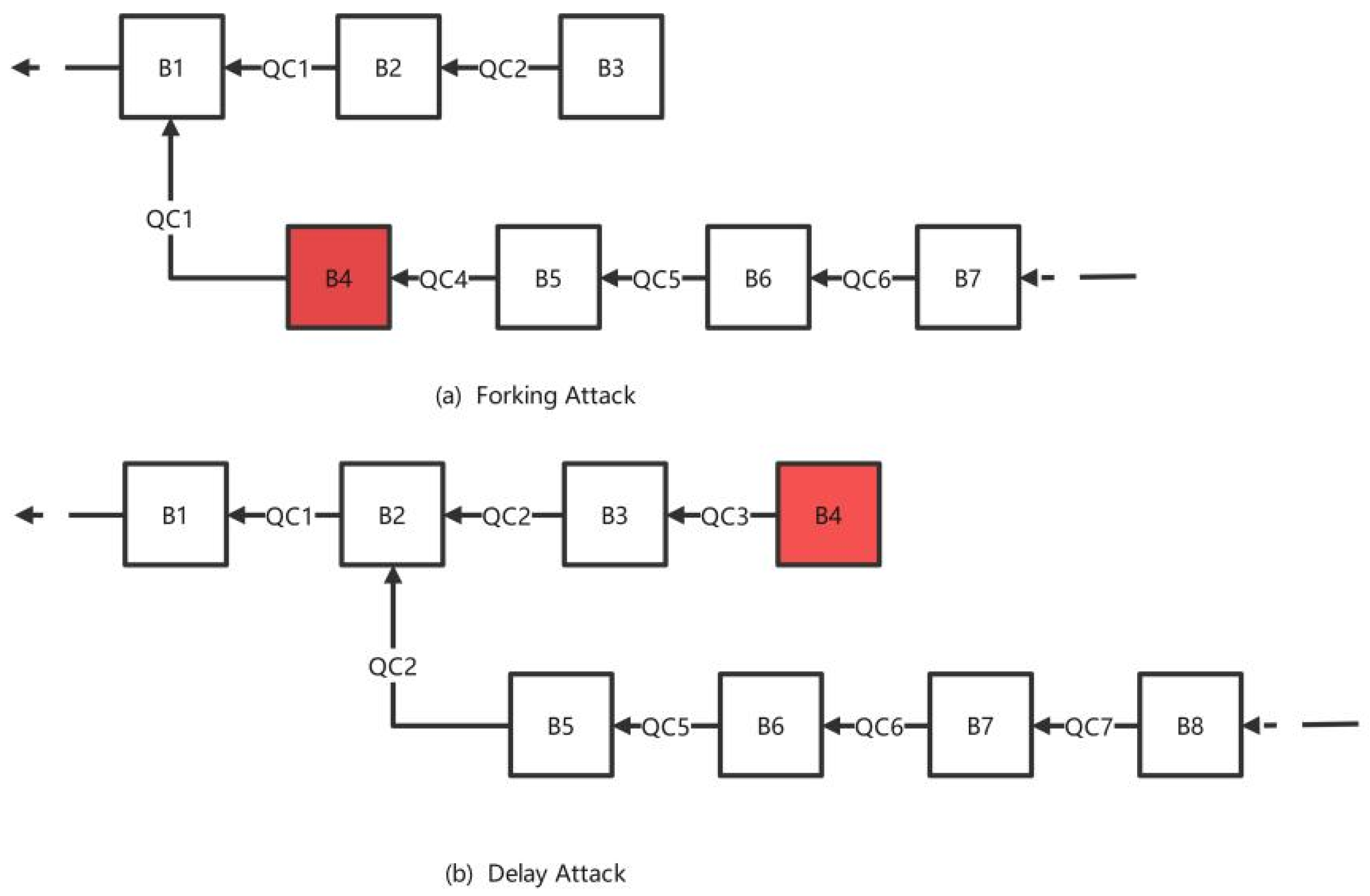
Forking attack [29] and delay attack [30] refer to a type of attack launched by the leader node in a consensus protocol, which can result in the appearance of invalid blocks, which will increase the delay of consensus and reduce the throughput of the consensus protocol. Figure 4a shows an illustration of a forking attack in the HotStuff protocol. The leader node launches a forking attack at view 4 (which corresponds to block B4). Since only block B1 in view 1 generated LockedQC (QC1) at this time, B4 can be connected after B1, causing a fork. Subsequent blocks will be connected after B4, and block 2 (B2) and block 3 (B3) will be discarded as a small fork of the entire blockchain and covered by block 4 and subsequent blocks. This will cause an increase in consensus delay and a decrease in throughput. Figure 4b shows an illustration of a delay attack in the HotStuff protocol. In view 4 (B4), the leader node launches a delay attack. The leader node does not take any action, and after the timeout, it switches to a new view. Only views 1 (B1) and 2 (B2) formed PrepareQC (QC1 and QC2) during the view switch, so the new block will be connected after B2, and block 3 (B3) and block 4 (B4) will be discarded, causing an increase in delay and a decrease in throughput.

The throughput of the HotStuff protocol was tested under network conditions with node size of 40, link bandwidth of 500 Mbps, and network delay between nodes of 50 ms. Figure 5 shows the variation diagram of the throughput of the HotStuff protocol under forking attack with the increase in the number of evil nodes. HotStuff throughput will drop significantly.

The QuickBFT protocol can tolerate up to f Byzantine nodes in the system, with a total number of nodes n = 3f + 1. To counteract the performance degradation caused by the leader node being attacked, we need a probability model to ensure that non-Byzantine nodes are more likely to be selected as leader nodes. The leader node selection strategy for the QuickBFT consensus protocol can be defined as a multi-attribute decision problem, where the decision variables are the replica nodes, and each replica node being selected as a leader node is a decision scheme. The multi-attribute of the decision system can be represented using the Vague set method to indicate the uncertain information in the consensus protocol. We proposed a TOPSIS multi-attribute decision-making method based on Vague sets to select the leader node. The multi-attribute includes the delay of the main node’s consensus, the reputation value of the node, CPU usage rate, and remaining bandwidth, and we built Vague sets on the four attributes to represent the membership degree and uncertainty of each attribute. We proposed an improved method for attribute weight determination, and we used the TOPSIS method to calculate the distances of each replica node from the positive ideal solution and negative ideal solution. And we calculate the comprehensive evaluation index of each node. Based on the comprehensive evaluation index, we calculate the probability that each replica node is selected as the leader node, and based on the probability, we calculate the new leader node and initiate a new round of consensus. We need two rounds of broadcast to synchronize information among nodes, and the rest of the calculations are performed locally on each node. In Section 4.1, we introduce the Vague set representation method for each attribute indicator. In Section 4.2, we introduce the synchronization scheme for each attribute information. In Section 4.3, we introduce the method of determining the goal weight. In Section 4.4, we introduce the TOPSIS method based on the Vague set, and in Section 4.5, we provide the process of the algorithm.

4.1. Vague Sets Representation of Attribute Index

In the QuickBFT protocol, we construct a Vague set using four attributes, namely consensus latency, node reputation, node CPU usage, and node bandwidth. We will introduce the Vague set representation of these four properties separately.

• Vague set representation of consensus delay

Consensus delay refers to the total time it takes for a round of consensus to complete, specifically from the start of the prepare stage to the end of the decide stage. Let us assume there are n nodes in total, with leader node l and replica node r. The consensus delay that replica node r calculates for this round can be expressed as follows:

$${\mathrm{D}\mathrm{e}\mathrm{l}\mathrm{a}\mathrm{y}}_{\mathrm{r}\mathrm{l}}={\mathrm{D}\mathrm{E}\mathrm{C}\mathrm{I}\mathrm{D}\mathrm{E}}_{\mathrm{r}\mathrm{l}}-{\mathrm{P}\mathrm{R}\mathrm{E}\mathrm{P}\mathrm{A}\mathrm{R}\mathrm{E}}_{\mathrm{r}\mathrm{l}}\{\mathrm{r}\in \mathrm{n},\mathrm{l}\in \mathrm{n}\}$$

(6)

Each replica node independently calculates the delay of a round of consensus and votes based on the consensus delay. The voting result has three types of values: V_a represents that the round of consensus is completed normally within the normal time, which can be considered as a vote of approval in the voting model; that is, the replica node believes that the leader node of this round of consensus is an honest node; V_w represents that the round of consensus is completed normally, but the consensus delay is significantly greater than the average consensus delay of other views, which can be considered as an abstaining vote in the voting model; V_o represents that the round of consensus has not been completed and triggered the timeout, which can be considered as a vote of disapproval in the voting model, that is, the replica node believes that the leader node of this round of consensus is a Byzantine node. Let V_rl represent the voting information of replica node r to leader node l:

$${\mathrm{V}}_{\mathrm{r}\mathrm{l}}=\left\{\begin{array}{c}{\mathrm{V}}_{\mathrm{a}},{\mathrm{D}\mathrm{e}\mathrm{l}\mathrm{a}\mathrm{y}}_{\mathrm{r}\mathrm{l}}<=\mathsf{\delta }·\frac{\sum _{\mathrm{i}=0}^{\mathrm{n}-1}{\mathrm{D}\mathrm{e}\mathrm{l}\mathrm{a}\mathrm{y}}_{\mathrm{r}\mathrm{i}}}{\mathrm{n}}\hfill \\ {\mathrm{V}}_{\mathrm{w}},{\mathrm{D}\mathrm{e}\mathrm{l}\mathrm{a}\mathrm{y}}_{\mathrm{r}\mathrm{l}}>\mathsf{\delta }·\frac{\sum _{\mathrm{i}=0}^{\mathrm{n}-1}{\mathrm{D}\mathrm{e}\mathrm{l}\mathrm{a}\mathrm{y}}_{\mathrm{r}\mathrm{i}}}{\mathrm{n}}\hfill \\ {\mathrm{V}}_{\mathrm{o}},{\mathrm{D}\mathrm{e}\mathrm{l}\mathrm{a}\mathrm{y}}_{\mathrm{r}\mathrm{l}}\mathrm{t}\mathrm{i}\mathrm{m}\mathrm{e}\mathrm{d}\mathrm{o}\mathrm{u}\mathrm{t}\hfill \end{array}\right.$$

(7)

After n rounds of consensus, the voting information on a replica node can be composed into a voting set:

$${\mathrm{V}}_{\mathrm{r}}=\left({\mathrm{V}}_{\mathrm{r}0},{\mathrm{V}}_{\mathrm{r}1},\dots {\mathrm{V}}_{\mathrm{r}(\mathrm{n}-1)}\right)$$

(8)

Each node broadcasts its own set of votes, and honest nodes construct a set of all nodes’ votes after receiving 2f + 1 vote messages:

$$\mathrm{V}=\begin{array}{ccc}{\mathrm{V}}_{00}& {\mathrm{V}}_{01}& \dots {\mathrm{V}}_{0(\mathrm{n}-1)}\\ ⋮& ⋮& ⋮\\ {\mathrm{V}}_{(\mathrm{n}-1)0}& {\mathrm{V}}_{(\mathrm{n}-1)1}& {\dots \mathrm{V}}_{(\mathrm{n}-1)(\mathrm{n}-1)}\end{array}$$

(9)

Then, the Vague set of the consensus delay of each replica node l when it serves as the leader node can be expressed as follows:

$$\begin{array}{c}{\mathrm{V}\mathrm{a}\mathrm{g}\mathrm{u}\mathrm{e}}_{\mathrm{l}}=({\mathrm{t}}_{\mathrm{l}},1-{\mathrm{f}}_{\mathrm{l}})\\ {\mathrm{t}}_{\mathrm{l}}=\frac{\mathrm{n}\mathrm{u}\mathrm{m}({{\mathrm{V}}_{\mathrm{i}\mathrm{l}}=\mathrm{V}}_{\mathrm{a}}),\mathrm{i}\in (0,\dots ,\mathrm{n}-1)}{\mathrm{n}}\\ {\mathrm{f}}_{\mathrm{l}}=\frac{\mathrm{n}\mathrm{u}\mathrm{m}({{\mathrm{V}}_{\mathrm{i}\mathrm{l}}=\mathrm{V}}_{\mathrm{o}}),\mathrm{i}\in (0,\dots ,\mathrm{n}-1)}{\mathrm{n}}\end{array}$$

(10)

The t_l represents the degree to which node l is a trustworthy leader, while f_l represents the degree to which node l is a Byzantine leader. The uncertainty of node l’s affiliation is represented by 1 − t_l − f_l.

2.

Vague set representation of node reputation values

The reputation value attribute of a node refers to the evaluation index of the leader node for replica nodes, similar to the representation method of the consensus delay Vague set. V_a represents the approval vote, indicating that the leader node received the voting information of the replica node within the specified time. V_w represents the abstaining vote, indicating that the leader node received the voting information of the replica node after exceeding the specified time, and V_o represents the opposing vote, indicating that the leader node did not receive the voting information of the replica node.

Assuming that the reputation value is represented by R, after n rounds of consensus, the reputation values of other replica nodes on a leader node l can be composed into a reputation value set:

$${\mathrm{R}}_{\mathrm{l}}=\left({\mathrm{R}}_{0\mathrm{l}},{\mathrm{R}}_{1\mathrm{l}},\dots {\mathrm{R}}_{(\mathrm{n}-1)\mathrm{l}}\right)$$

(11)

Each node broadcasts its own set of reputation values, and honest nodes can construct a set of reputation values for all nodes after receiving 2f + 1 sets of reputation values information.

Let r represent a replica node, then the Vague set of reputation values of the replica node r can be expressed as follows:

$$\begin{array}{c}{\mathrm{V}\mathrm{a}\mathrm{g}\mathrm{u}\mathrm{e}}_{\mathrm{r}}=({\mathrm{t}}_{\mathrm{r}},1-{\mathrm{f}}_{\mathrm{r}})\\ {\mathrm{t}}_{\mathrm{r}}=\frac{\mathrm{n}\mathrm{u}\mathrm{m}({{\mathrm{R}}_{\mathrm{r}\mathrm{i}}=\mathrm{V}}_{\mathrm{a}}),\mathrm{i}\in (0,\dots ,\mathrm{n}-1)}{\mathrm{n}}\\ {\mathrm{f}}_{\mathrm{r}}=\frac{\mathrm{n}\mathrm{u}\mathrm{m}({{\mathrm{R}}_{\mathrm{r}\mathrm{i}}=\mathrm{V}}_{\mathrm{o}}),\mathrm{i}\in (0,\dots ,\mathrm{n}-1)}{\mathrm{n}}\end{array}$$

(12)

3.

Vague set representation of node CPU utilization

The CPU usage rate of a node is related to the efficiency of signature aggregation and verification when the node serves as a leader node. Therefore, the selection strategy for the leader node should tend to choose nodes with lower CPU usage rates.

During the n rounds of consensus, node r samples the CPU usage rate and obtains a set of CPU usage rates for nodes over a period of time t:

$$\mathrm{U}\mathrm{R}=({\mathrm{U}\mathrm{R}}_1,\dots ,{\mathrm{U}\mathrm{R}}_{\mathrm{t}-1},{\mathrm{U}\mathrm{R}}_{\mathrm{t}}),\mathrm{U}\mathrm{R}\to \left[\mathrm{0,1}\right]$$

(13)

The Vague set of CPU usage of node r can be expressed as follows:

$$\begin{array}{c}{\mathrm{V}\mathrm{a}\mathrm{g}\mathrm{u}\mathrm{e}}_{\mathrm{U}\mathrm{R}}=({\mathrm{t}}_{\mathrm{r}},1-{\mathrm{f}}_{\mathrm{r}})\\ {\mathrm{t}}_{\mathrm{r}}=1-\frac{{\sum }_{\mathrm{i}=1}^{\mathrm{t}}{\mathrm{U}\mathrm{R}}_{\mathrm{i}}}{\mathrm{t}}\\ {\mathrm{f}}_{\mathrm{r}}=\mathrm{m}\mathrm{i}\mathrm{n}({\mathrm{U}\mathrm{R}}_{\mathrm{i}}),\mathrm{i}\in [1,\mathrm{t}]\end{array}$$

(14)

Because nodes with lower CPU utilization are more likely to be chosen as leader nodes, t_r can be interpreted as the average CPU idle rate of node r in time period t, f_r can be interpreted as the minimum CPU utilization rate of node r in time period t, and 1 − f_r can be interpreted as the maximum CPU idle rate of node r in time period t.

4.

Vague set representation of node bandwidth

Assuming that the total bandwidth of all nodes is the same since the network connection between the leader node and the replica node is in a point-to-point mode, the communication volume of the leader node will linearly increase as the number of nodes increases. The selection strategy for the leader node should tend to choose nodes with higher remaining bandwidth. Let the total bandwidth of a node be BW, and during the n rounds of consensus, node r samples the network throughput over a period of time t and obtains a set of network throughput measurements over that period:

$$\mathrm{B}=({\mathrm{B}}_1,\dots ,{\mathrm{B}}_{\mathrm{t}-1},{\mathrm{B}}_{\mathrm{t}}),\mathrm{B}\to \left[0,\mathrm{B}\mathrm{W}\right]$$

(15)

Then, the Vague set of bandwidth of node r can be expressed as follows:

$$\begin{array}{c}{\mathrm{V}\mathrm{a}\mathrm{g}\mathrm{u}\mathrm{e}}_{\mathrm{B}}=({\mathrm{t}}_{\mathrm{r}},1-{\mathrm{f}}_{\mathrm{r}})\\ {\mathrm{t}}_{\mathrm{r}}=\frac{\mathrm{B}\mathrm{W}-\frac{{\sum }_{\mathrm{i}=1}^{\mathrm{t}}{\mathrm{B}}_{\mathrm{i}}}{\mathrm{t}}}{\mathrm{B}\mathrm{W}}\\ {\mathrm{f}}_{\mathrm{r}}=\frac{\mathrm{m}\mathrm{i}\mathrm{n}({\mathrm{B}}_{\mathrm{i}})}{\mathrm{B}\mathrm{W}},\mathrm{i}\in [1,\mathrm{t}]\end{array}$$

(16)

Because nodes with higher remaining bandwidth should have a higher probability of being chosen as the leader node, t_r can be interpreted as the ratio of the average remaining bandwidth of a node r over a period of time t to the total bandwidth, f_r can be interpreted as the ratio of the minimum network throughput of a node r over a period of time t to the total bandwidth, 1 − f_r can be interpreted as the ratio of the maximum remaining bandwidth of a node r over a period of time t to the total bandwidth.

4.2. Attribute Information Synchronization Scheme

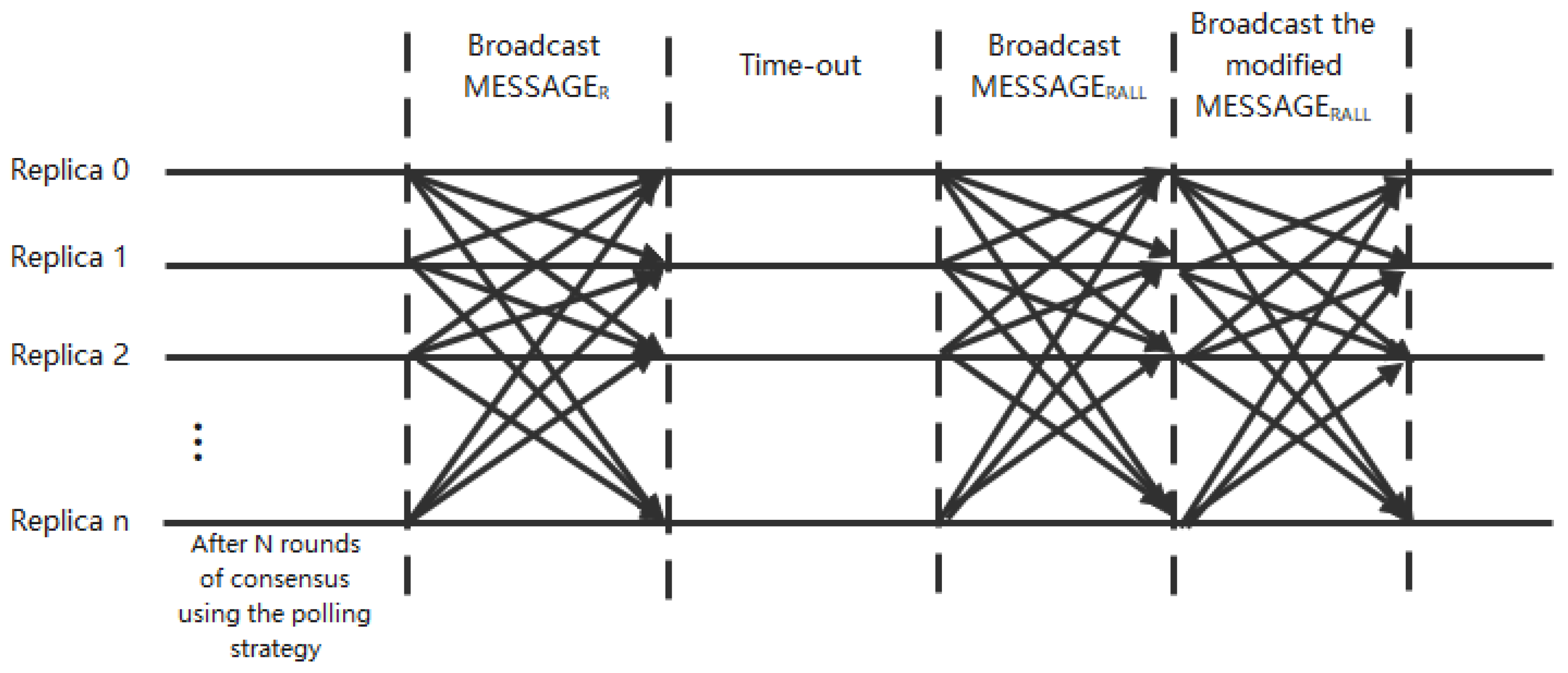
In order to ensure that the computational results of the replica nodes are consistent, we need to ensure that the attribute information of the replica nodes is the same. Therefore, we need to perform three rounds of broadcast communication and remove any possible noise before selecting the leader node.

After n rounds of consensus using the polling scheme, the format of all the attribute information of a node r is as follows:

$${\mathrm{M}\mathrm{E}\mathrm{S}\mathrm{S}\mathrm{A}\mathrm{G}\mathrm{E}}_{\mathrm{r}}=\{({\mathrm{V}}_{\mathrm{r}0},{\mathrm{V}}_{\mathrm{r}1},\dots {\mathrm{V}}_{\mathrm{r}(\mathrm{n}-1)}),({\mathrm{R}}_{0\mathrm{r}},{\mathrm{R}}_{1\mathrm{r}},\dots {\mathrm{R}}_{(\mathrm{n}-1)\mathrm{r}}),{\mathrm{V}\mathrm{a}\mathrm{g}\mathrm{u}\mathrm{e}}_{\mathrm{U}\mathrm{R}},{\mathrm{V}\mathrm{a}\mathrm{g}\mathrm{u}\mathrm{e}}_{\mathrm{B}}\}$$

(17)

In which V represents the consensus delay measured by node r in each round, R represents the reputation value of other nodes measured by node r when it serves as a leader, ${\mathrm{V}\mathrm{a}\mathrm{g}\mathrm{u}\mathrm{e}}_{\mathrm{U}\mathrm{R}}$ represents a Vague set representation of the CPU usage of the node, and ${\mathrm{V}\mathrm{a}\mathrm{g}\mathrm{u}\mathrm{e}}_{\mathrm{B}}$ represents a Vague set representation of the bandwidth of the node. After n rounds of consensus using the polling scheme, each replica node broadcasts its local ${\mathrm{M}\mathrm{E}\mathrm{S}\mathrm{S}\mathrm{A}\mathrm{G}\mathrm{E}}_{\mathrm{r}}$ information. When an honest node receives information from other nodes, it constructs a Vague set of consensus delay and reputation values according to the method described in Section 4.1. It sets a timeout limit, and for information that has not been received within the time limit, it uses the default value instead. At this point, each node has gathered all the information from the other nodes:

$${\mathrm{M}\mathrm{E}\mathrm{S}\mathrm{S}\mathrm{A}\mathrm{G}\mathrm{E}}_{\mathrm{r}\mathrm{a}\mathrm{l}\mathrm{l}}=\left\{\begin{array}{ccc}({\mathrm{V}}_{00},{\mathrm{V}}_{01},\dots {\mathrm{V}}_{0(\mathrm{n}-1)})& \begin{array}{cc}({\mathrm{R}}_{00},{\mathrm{R}}_{10},\dots {\mathrm{R}}_{(\mathrm{n}-1)0})& {\mathrm{V}\mathrm{a}\mathrm{g}\mathrm{u}\mathrm{e}}_{\mathrm{U}\mathrm{R}0}\end{array}& {\mathrm{V}\mathrm{a}\mathrm{g}\mathrm{u}\mathrm{e}}_{\mathrm{B}0}\\ \begin{array}{c}({\mathrm{V}}_{10},{\mathrm{V}}_{11},\dots {\mathrm{V}}_{1(\mathrm{n}-1)})\\ ⋮\end{array}& \begin{array}{cc}\begin{array}{c}({\mathrm{R}}_{01},{\mathrm{R}}_{11},\dots {\mathrm{R}}_{(\mathrm{n}-1)1})\\ ⋮\end{array}& \begin{array}{c}{\mathrm{V}\mathrm{a}\mathrm{g}\mathrm{u}\mathrm{e}}_{\mathrm{U}\mathrm{R}1}\\ ⋮\end{array}\end{array}& \begin{array}{c}{\mathrm{V}\mathrm{a}\mathrm{g}\mathrm{u}\mathrm{e}}_{\mathrm{B}1}\\ ⋮\end{array}\\ ({\mathrm{V}}_{(\mathrm{n}-1)0},{\mathrm{V}}_{(\mathrm{n}-1)1},\dots {\mathrm{V}}_{(\mathrm{n}-1)(\mathrm{n}-1)})& \begin{array}{cc}({\mathrm{R}}_{0(\mathrm{n}-1)},{\mathrm{R}}_{1(\mathrm{n}-1)},\dots {\mathrm{R}}_{(\mathrm{n}-1)(\mathrm{n}-1)})& {\mathrm{V}\mathrm{a}\mathrm{g}\mathrm{u}\mathrm{e}}_{\mathrm{U}\mathrm{R}\mathrm{n}-1}\end{array}& {\mathrm{V}\mathrm{a}\mathrm{g}\mathrm{u}\mathrm{e}}_{\mathrm{B}\mathrm{n}-1}\end{array}\right\}$$

(18)

Each node broadcasts the MESSAGErall information it has collected after receiving at least 2f + 1 messages and exceeding the timeout limit. Since the number of honest nodes in the system is greater than 2f + 1, it can be assumed that more than 2f + 1 rows of the MESSAGErall information received from other nodes are consistent with the local MESSAGErall information. Compare the information of all honest nodes, replace the rows with inconsistent data with default values, and after collecting 2f + 1 MESSAGErall information and replacing the rows with inconsistent data. The node broadcasts the modified MESSAGErall information again. After receiving 2f + 1 modified MESSAGErall information, the node begins the calculation of selecting the leader node. The synchronization scheme for attribute information communication is shown in Figure 6.

4.3. The TOPSIS Method Based on Vague Sets

The TOPSIS method ranks solutions by calculating their relative proximity to the ideal solution. When applying the TOPSIS method for solution selection, our goal is to find the solution that is closest to the positive ideal solution (PIS) and the one that is farthest from the negative ideal solution (NIS). The positive ideal solution is the one with the maximum benefit attribute value and the smallest cost attribute value among all feasible solutions. On the other hand, the negative ideal solution is the one with the minimum benefit attribute value and the largest cost attribute value among all feasible solutions. In the TOPSIS method, these two solutions serve as reference points, and the distance to them is used to measure the quality of the solutions. We propose a TOPSIS method based on Vague sets [31], combining the distance of Vague sets to calculate the distances of each candidate solution to the positive and negative ideal solutions and then sorting them based on the distances to determine the priority of each solution. The solution that is closest to PIS and farthest from NIS is the optimal solution.

Definition 2.

Let A be the set of decision alternatives {A1, A2, …, Am} and C be the set of attribute indicators {C1, C2, …, Cn}. The positive ideal solution A⁺ and negative ideal solution A⁻ of the solution set that satisfies the constraint conditions of the attribute set are as follows:

$$\begin{array}{c}{\mathrm{A}}^{+}=\{(\mathrm{C}1,\left[\mathrm{1,1}\right]),(\mathrm{C}2,\left[\mathrm{1,1}\right]),\dots (\mathrm{C}\mathrm{n},\left[\mathrm{1,1}\right])\}\\ {\mathrm{A}}^{-}=\{(\mathrm{C}1,\left[\mathrm{0,0}\right]),(\mathrm{C}2,\left[\mathrm{0,0}\right]),\dots (\mathrm{C}\mathrm{n},\left[\mathrm{0,0}\right])\}\end{array}$$

(19)

In the QuickBFT protocol, the attribute indicator set refers to the consensus delay, node reputation, CPU usage, and bandwidth of nodes, which are represented by Vague sets. The choice of decision scheme A1 can be interpreted as choosing replica node 1 as the leader node. The definitions of positive and negative ideal schemes conform to traditional mathematical thinking, but the degrees of membership of 0 and 1 are two extreme forms, and actual schemes are often difficult to meet. Based on this, we provide the following improved definition of positive and negative ideal schemes.

Definition 3.

Let A be the set of decision alternatives {A1, A2, …, Am}, C be the set of attribute indicators {C1, C2, …, Cn}, and the positive and negative ideal solutions be as follows:

$$\begin{array}{c}{\mathrm{A}}_{\mathrm{i}}^{+}=\mathrm{m}\mathrm{a}\mathrm{x}\{(\mathrm{C}1,[{\mathrm{t}}_{\mathrm{i}1},1-{\mathrm{f}}_{\mathrm{i}1}]),(\mathrm{C}2,[{\mathrm{t}}_{\mathrm{i}2},1-{\mathrm{f}}_{\mathrm{i}2}]),\dots (\mathrm{C}\mathrm{n},[{\mathrm{t}}_{\mathrm{i}\mathrm{n}},1-{\mathrm{f}}_{\mathrm{i}\mathrm{n}}])\},\mathrm{i}=1,2,\dots ,\mathrm{m}\\ {\mathrm{A}}_{\mathrm{i}}^{-}=\mathrm{m}\mathrm{i}\mathrm{n}\{(\mathrm{C}1,[{\mathrm{t}}_{\mathrm{i}1},1-{\mathrm{f}}_{\mathrm{i}1}]),(\mathrm{C}2,[{\mathrm{t}}_{\mathrm{i}2},1-{\mathrm{f}}_{\mathrm{i}2}]),\dots (\mathrm{C}\mathrm{n},[{\mathrm{t}}_{\mathrm{i}\mathrm{n}},1-{\mathrm{f}}_{\mathrm{i}\mathrm{n}}])\},\mathrm{i}=1,2,\dots ,\mathrm{m}\end{array}$$

(20)

We will denote the Vague values corresponding to the positive and negative ideal solutions as VPIS and VNIS, respectively.

Definition 4.

Let C = {C1, C2, …, Cn} be a set of attribute indicators, and let w = {w1, w2, …, wn} be the corresponding weight coefficients. The weighted distance between the solution A_i and the positive ideal solution is defined as follows:

$${\mathrm{d}}_{\mathrm{i}}^{+}=\mathrm{d}({\mathrm{A}}_{\mathrm{i}},{\mathrm{A}}_{\mathrm{i}}^{+})=\sqrt{\frac{1}{4\mathrm{n}}\sum _{\mathrm{j}=1}^{\mathrm{n}}{\mathrm{w}}_{\mathrm{j}}\mathrm{d}(({\mathrm{t}}_{\mathrm{i}\mathrm{j}},1-{\mathrm{f}}_{\mathrm{i}\mathrm{j}}),\mathrm{V}\mathrm{P}\mathrm{I}\mathrm{S})},\hspace{1em}\mathrm{i}=1,2,\dots ,\mathrm{m}$$

(21)

The weighted distance between the A_i solution and the negative ideal solution is defined as follows:

$${\mathrm{d}}_{\mathrm{i}}^{-}=\mathrm{d}({\mathrm{A}}_{\mathrm{i}},{\mathrm{A}}_{\mathrm{i}}^{-})=\sqrt{\frac{1}{4\mathrm{n}}\sum _{\mathrm{j}=1}^{\mathrm{n}}{\mathrm{w}}_{\mathrm{j}}\mathrm{d}(({\mathrm{t}}_{\mathrm{i}\mathrm{j}},1-{\mathrm{f}}_{\mathrm{i}\mathrm{j}}),\mathrm{V}\mathrm{N}\mathrm{I}\mathrm{S})},\hspace{1em}\mathrm{i}=1,2,\dots ,\mathrm{m}$$

(22)

Definition 5.

Based on the definitions of $d_i^{+}$ and $d_i^{-}$, we define the comprehensive evaluation index of each decision option (replica node) as follows:

$$\mathsf{\mu }({\mathrm{A}}_{\mathrm{i}})=\frac{{\mathrm{d}}_{\mathrm{i}}^{-}}{{\mathrm{d}}_{\mathrm{i}}^{-}+{\mathrm{d}}_{\mathrm{i}}^{+}},\mathrm{i}=1,2,\dots ,\mathrm{m}$$

(23)

The larger the comprehensive evaluation index $\mu (A_i)$ is, the closer the solution A_i is to the positive ideal solution and away from the negative ideal solution at the same time. Therefore, the size of $\mu (A_i)$ represents the degree to which the node belongs to the honest node. According to the comprehensive evaluation index of each replica node, the probability of the replica node being selected as the leader node can be calculated.

Definition 6.

According to the definition of $\mu (A_i)$, $\mu (A_i)$ represents the degree to which a node belongs to an honest node, then the probability that replica node i is chosen to become the leader node is as follows:

$$\mathrm{P}({\mathrm{A}}_{\mathrm{i}})=\frac{\mathsf{\mu }({\mathrm{A}}_{\mathrm{i}})}{\sum _{\mathrm{j}=1}^{\mathrm{m}}\mathsf{\mu }({\mathrm{A}}_{\mathrm{i}})},\hspace{1em}\mathrm{i}=1,2,\dots ,\mathrm{m}$$

(24)

We use VRF (Verifiable Random Function) to generate a random number. VRF is a cryptographic primitive that allows anyone to generate a seemingly random output without a private key while allowing the verifier with the private key to prove that the output was generated from a specific input. VRF (verifiable random function) has pseudorandomness, verifiability, and uniqueness. In each round of consensus, the random number seed of the previous round’s VRF algorithm is used as the random number seed for the next round of consensus. In the QuickBFT protocol, during the prepare phase, the leader node generates the seed and random number for the current round of consensus based on the seed of the previous round’s VRF function and then sends them to the replica nodes for validation of the random number seed and random number. The random number is used to determine the selection of the next round’s leader node. The definition of the random number seed is as follows:

$${\mathrm{s}\mathrm{e}\mathrm{e}\mathrm{d}}_{\mathrm{r}}=\mathrm{H}({\mathrm{s}\mathrm{e}\mathrm{e}\mathrm{d}}_{\mathrm{r}-1}||{\mathsf{\sigma }}_{\mathrm{r}-1})$$

(25)

The seed of round r is determined by the seed of round r − 1 and the aggregated signature ${\sigma }_{r-1}$. The aggregated signature is formed by aggregating the signatures of more than 2f + 1 replica nodes received by the leader node during the preparation stage, and the replica nodes determine the new leader node based on the random numbers generated by the VRF and send the NEWVIEW message to start a new round of consensus.

4.4. Method of Determining Target Weight

In Definition 4, we mentioned that the weight coefficient of attribute indicator C is w. In multi-attribute decision-making problems, the proportion of weights of each attribute has an impact on the final decision-making solution. Determining the weights of each attribute objectively is an important issue. This paper proposes an improved weight determination method as follows:

The basic idea of using the TOPSIS method to solve problems is that the attribute weight w_j should be chosen in such a way that the final decision solution A_i of the scheme is the maximum weighted distance from the positive ideal solution and the minimum weighted distance from the negative ideal solution. Therefore, the following single-objective programming model can be established:

$$\left\{\begin{array}{c}\mathrm{m}\mathrm{i}\mathrm{n}{\displaystyle \sum _{\mathrm{i}=1}^{\mathrm{m}}}{\displaystyle \sum _{\mathrm{j}=1}^{\mathrm{n}}}{{\mathrm{w}}_{\mathrm{j}}}^2{\mathrm{d}}^2({\mathrm{A}}_{\mathrm{i}},{\mathrm{A}}_{\mathrm{i}}^{-}),\mathrm{m}\mathrm{a}\mathrm{x}{\displaystyle \sum _{\mathrm{i}=1}^{\mathrm{m}}}{\displaystyle \sum _{\mathrm{j}=1}^{\mathrm{n}}}{{\mathrm{w}}_{\mathrm{j}}}^2{\mathrm{d}}^2({\mathrm{A}}_{\mathrm{i}},{\mathrm{A}}_{\mathrm{i}}^{+})\hfill \\ \mathrm{s}.\mathrm{t}.\hspace{1em}{\displaystyle \sum _{\mathrm{j}=1}^{\mathrm{n}}}{\mathrm{w}}_{\mathrm{j}}=1,0\le {\mathrm{w}}_{\mathrm{j}}\le 1\hfill \end{array}\right.$$

(26)

Perform normalization:

$$\left\{\begin{array}{c}\mathrm{m}\mathrm{i}\mathrm{n}({\displaystyle \sum _{\mathrm{i}=1}^{\mathrm{m}}}{\displaystyle \sum _{\mathrm{j}=1}^{\mathrm{n}}}{{\mathrm{w}}_{\mathrm{j}}}^2({\mathrm{d}}^2({\mathrm{A}}_{\mathrm{i}},{\mathrm{A}}_{\mathrm{i}}^{-})-{\mathrm{d}}^2({\mathrm{A}}_{\mathrm{i}},{\mathrm{A}}_{\mathrm{i}}^{+})))\hfill \\ \mathrm{s}.\mathrm{t}.{\displaystyle \sum _{\mathrm{j}=1}^{\mathrm{n}}}{\mathrm{w}}_{\mathrm{j}}=1,0\le {\mathrm{w}}_{\mathrm{j}}\le 1\hfill \end{array}\right.$$

(27)

The problem is transformed into finding the optimal solution of the above objective programming model, which can be solved by constructing a Lagrange function $\mathrm{L}(\mathrm{w},\mathsf{\gamma })$:

$$\mathrm{L}(\mathrm{w},\mathsf{\gamma })={\displaystyle \sum _{\mathrm{i}=1}^{\mathrm{m}}}{\displaystyle \sum _{\mathrm{j}=1}^{\mathrm{n}}}{{\mathrm{w}}_{\mathrm{j}}}^2({\mathrm{d}}^2({\mathrm{A}}_{\mathrm{i}},{\mathrm{A}}_{\mathrm{i}}^{-})-{\mathrm{d}}^2({\mathrm{A}}_{\mathrm{i}},{\mathrm{A}}_{\mathrm{i}}^{+}))+\mathsf{\gamma }({\displaystyle \sum _{\mathrm{j}=1}^{\mathrm{n}}}{\mathrm{w}}_{\mathrm{j}}-1)$$

(28)

Let $\frac{\partial \mathrm{L}}{\partial \mathsf{\gamma }}=0$ and $\frac{\partial \mathrm{L}}{\partial {\mathrm{w}}_{\mathrm{j}}}=0$, then we have the following:

$$\left\{\begin{array}{c}2{\displaystyle \sum _{\mathrm{i}=1}^{\mathrm{m}}}{\displaystyle \sum _{\mathrm{j}=1}^{\mathrm{n}}}{\mathrm{w}}_{\mathrm{j}}({\mathrm{d}}^2({\mathrm{A}}_{\mathrm{i}},{\mathrm{A}}_{\mathrm{i}}^{-})-{\mathrm{d}}^2({\mathrm{A}}_{\mathrm{i}},{\mathrm{A}}_{\mathrm{i}}^{+}))+\mathsf{\gamma }=0\hfill \\ {\displaystyle \sum _{\mathrm{j}=1}^{\mathrm{n}}}{\mathrm{w}}_{\mathrm{j}}=1,0\le {\mathrm{w}}_{\mathrm{j}}\le 1\hfill \end{array}\right.$$

(29)

Solve the equation to calculate the following attribute indicators:

$${\mathrm{w}}_{\mathrm{j}}=\frac{\frac{1}{\sum _{\mathrm{j}=1}^{\mathrm{n}}\frac{1}{\sum _{\mathrm{i}=1}^{\mathrm{m}}({\mathrm{d}}^2({\mathrm{A}}_{\mathrm{i}},{\mathrm{A}}_{\mathrm{i}}^{-})-{\mathrm{d}}^2({\mathrm{A}}_{\mathrm{i}},{\mathrm{A}}_{\mathrm{i}}^{+}))}}}{\sum _{\mathrm{i}=1}^{\mathrm{m}}({\mathrm{d}}^2({\mathrm{A}}_{\mathrm{i}},{\mathrm{A}}_{\mathrm{i}}^{-})-{\mathrm{d}}^2({\mathrm{A}}_{\mathrm{i}},{\mathrm{A}}_{\mathrm{i}}^{+}))},\hspace{1em}\mathrm{j}=\mathrm{1,2},\dots ,\mathrm{n}$$

(30)

4.5. Algorithm Process

The steps of the algorithm for selecting the leader node based on the Vague set and TOPSIS method are as follows:

• After the QuickBFT protocol starts, the module for selecting the leader node first initializes;
• After initialization, QuickBFT conducts N (N = number of nodes) rounds of consensus based on the round-robin leader selection strategy and then constructs attribute indicators based on the Vague set. The attribute indicators include consensus delay, node reputation value, node CPU utilization, and node bandwidth. The CPU utilization and bandwidth of nodes can be represented by directly constructing a Vague set, while the consensus delay and reputation value attributes of nodes require the synchronization of attribute information among nodes before constructing a Vague set to represent;
• According to the attribute information synchronization scheme described in Section 4.2, the nodes use a three-round broadcast method to synchronize their attribute information and construct a Vague set of all attribute information to ensure consistency of the attribute information of honest nodes;
• Each node performs the computation of selecting the leader node locally and calculates the positive ideal solution (VPIS) and negative ideal solution (VNIS) according to the definition in Section 4.3;
• Calculate the weights of each attribute according to the method outlined in Section 4.4;
• According to the weights of each attribute and the definition in Section 4.3, the weighted distances between each replica node and VPIS and VNIS are calculated;
• The comprehensive evaluation index of each replica node is calculated based on the distance between each replica node and the positive and negative ideal solutions, and the probability of each node being selected as the leader node is calculated;
• A random number is generated according to the VRF verifiable random function, and each node selects the leader node for the next round of consensus according to the probability in Step 7 and initiates voting;
• If the remainder of the view ID divided by the number of nodes is not zero, proceed to step 8, where the seed for the next round of consensus is determined by the seed of the previous round of consensus and the aggregated signature, ensuring the randomness of the seed;
• If the remainder of the view ID divided by the number of nodes is zero (after N rounds of consensus), proceed to step 2.

The leader selection algorithm in QuickBFT requires broadcasting each node’s attribute information, resulting in a communication complexity of O(n²). However, since the leader selection algorithm performs calculations in n rounds, the final communication complexity is O(n).

5. Proof of Safety and Liveness

In a distributed system, the order of concurrent instructions needs to be agreed upon by all processors. Otherwise, a misordered sequence of concurrent instructions can cause inconsistencies in processor states. Blockchain is a distributed system, and its most fundamental feature is the consensus mechanism. A distributed system’s consensus mechanism must meet the following two requirements:

• Safety [32]: The safety of consensus protocol refers to the fact that honest nodes in the system agree on the same value. In QuickBFT, the safety problem actually refers to whether there are conflicting branches in the system, i.e., to ensure that different honest nodes have the same branch;
• Liveness [33]: The liveness of a consensus protocol refers to the fact that if a consensus proposal is correct and sent to the consensus network, it will ultimately be confirmed in the consensus network. Liveness ensures that the consensus protocol will continue to operate without interruption due to node failures or other factors, thereby preventing the entire consensus process from being blocked and causing a decline in system performance.

According to the CAP [34] theory of distributed systems, it is impossible for a distributed system to simultaneously satisfy consistency, availability, and partition tolerance. According to the FLP [35] impossibility theorem, in an asynchronous communication environment, even if only one process fails, there is no algorithm that can guarantee that the non-failed processes achieve consistency. We can only assume that the consensus protocol is run on a partially synchronous network model for proof of safety and liveness.

5.1. Safety

In a distributed system with n replica nodes, each node maintains its own local tree, with 2f + 1 honest nodes maintaining essentially the same (except for the final few blocks) tree. In the three-phase QuickBFT protocol, replica nodes only cast a vote of approval for the leaf nodes on the successor branch of the PrepareQC node with the highest view sequence number on their local tree. We define that if the aggregated signature verification is successful, it proves that the QC is valid.

Lemma 1.

For any valid qc1 and qc2, where qc1.type = qc2.type, and the tree nodes corresponding to qc1 and qc2 conflict, it must be the case that qc1.viewNumber ! = qc2.viewNumber.

Proof of Lemma 1.

We use proof by contradiction to prove that, assuming qc1.viewNumber = qc2.viewNumber = v. Since an effective proof certificate QC is at least formed by 2f + 1 votes (polymerization signature), there must be a correct copy that voted twice in the same stage of view v. This is impossible because the pseudocode in Algorithm 2 in Section 3.3 allows voting for each stage in each view only once. □

The Safety Theorem. 

If a and b are two conflicting tree nodes, then they cannot both be committed by a correct replica.

Proof of Safety: 

It can be proved by contradiction. We define DecideQC of node a in the tree as qc1 and DecideQC of node b as qc2 since a and b are two conflicting nodes. According to Lemma 1, we have qc1.viewNumber ! = qc2.viewNumber. We assume that qc1.viewNumber < qc2.viewNumber, and node a has a lower height than node b, qc1.node = a, and qc2.node = b. Let qcs be the smallest valid PrepareQC certificate with a higher height than a and conflicting with a:

$$\begin{array}{c}\mathrm{E}(\mathrm{P}\mathrm{r}\mathrm{e}\mathrm{p}\mathrm{a}\mathrm{r}\mathrm{e}\mathrm{Q}\mathrm{C}):=(\mathrm{v}1<\mathrm{P}\mathrm{r}\mathrm{e}\mathrm{p}\mathrm{a}\mathrm{r}\mathrm{e}\mathrm{Q}\mathrm{C}.\mathrm{v}\mathrm{i}\mathrm{e}\mathrm{w}\mathrm{N}\mathrm{u}\mathrm{m}\mathrm{b}\mathrm{e}\mathrm{r}<\mathrm{v}2)\\ \cap (\mathrm{P}\mathrm{r}\mathrm{e}\mathrm{p}\mathrm{a}\mathrm{r}\mathrm{e}\mathrm{Q}\mathrm{C}.\mathrm{n}\mathrm{o}\mathrm{d}\mathrm{e}\mathrm{c}\mathrm{o}\mathrm{n}\mathrm{f}\mathrm{l}\mathrm{i}\mathrm{c}\mathrm{t}\mathrm{s}\mathrm{w}\mathrm{i}\mathrm{t}\mathrm{h}\mathrm{a}).\\ \mathrm{q}\mathrm{c}\mathrm{s}:={\mathrm{a}\mathrm{r}\mathrm{g}\mathrm{m}\mathrm{i}\mathrm{n}}_{\mathrm{P}\mathrm{r}\mathrm{e}\mathrm{p}\mathrm{a}\mathrm{r}\mathrm{e}\mathrm{Q}\mathrm{C}}\{\mathrm{P}\mathrm{r}\mathrm{e}\mathrm{p}\mathrm{a}\mathrm{r}\mathrm{e}\mathrm{Q}\mathrm{C}.\mathrm{v}\mathrm{i}\mathrm{e}\mathrm{w}\mathrm{N}\mathrm{u}\mathrm{m}\mathrm{b}\mathrm{e}\mathrm{r}|\mathrm{P}\mathrm{r}\mathrm{e}\mathrm{p}\mathrm{a}\mathrm{r}\mathrm{e}\mathrm{Q}\mathrm{C}\mathrm{i}\mathrm{s}\mathrm{v}\mathrm{a}\mathrm{l}\mathrm{i}\mathrm{d}\cap \mathrm{E}(\mathrm{P}\mathrm{r}\mathrm{e}\mathrm{p}\mathrm{a}\mathrm{r}\mathrm{e}\mathrm{Q}\mathrm{C})\}.\end{array}$$

(31)

As shown in Figure 7, here is a diagram of qc1, qc2, and qcs, a and b are two conflicting tree nodes:

qc1 and qc2 are valid DecideQC certificates, and QCS is a valid PrepareQC certificate. Algorithm 2 in Section 3.3 explains that a DecideQC is composed of 2f + 1 LockedQCs. In Algorithm 1 of Section 3.3, the SAFENODE function indicates that generating a PrepareQC requires 2f + 1 replicas to pass the SAFENODE verification simultaneously. Therefore, there must exist a public r such that when viewed from view v1, the LockedQC is set to qc1, and when qcs attempts to verify the SAFENODE function, it will discover that qcs does not satisfy either “qcs.node extends from qc1.node” or “qcs.justify.viewNumber > qc1.viewNumber”. This means that qcs cannot be generated, contradicting the assumption. We can prove by contradiction that it is impossible to have two conflicting transactions. □

5.2. Liveness

We first define that after a global stability time GST, there exists a bounded duration Tf such that if all replicas are still in view v during Tf and the leader node of view v is functioning normally, then the client’s proposal can eventually be executed.

Lemma 2.

If a functioning replica node has locked a view, i.e., locked the corresponding LockedQC, then at least f + 1 replica nodes have voted for the PrepareQC that matches the LockedQC.

Proof of Lemma 2.

If a replica node r has locked a LockedQC, then PrepareQC must have received 2f + 1 votes in the prepare phase according to Algorithm 2 in Section 3.3, since n ≥ 3f + 1, at least f + 1 normal running replica nodes must have voted for the PrepareQC that matches the LockedQC. □

Proof of Liveness. 

Starting from a new view, the leader node collects 2f + 1 NEWVIEW messages and calculates their HighQC, then broadcasts the Prepare message. Assuming that the highest locked QC among all replica nodes (including the leader node itself) is LockedQC1, based on Lemma 2, it can be known that at least f + 1 correct replica nodes have voted for a PrepareQC matching LockedQC1 in a view, and the value has been attached to the NEWVIEW message sent to the leader node. In these NEWVIEW messages, at least one will be accepted by the leader node and assigned to HighQC. Under the assumption conditions, all correct replica nodes are in a synchronized state in this view, and the leader node is an honest node. Therefore, all correct replica nodes will vote in the prepare stage, as the conditions in the SAFENODE function are met (i.e., the branch node is after the highest HighQC-corresponding tree node, and the new QC view is greater than the local LockedQC-corresponding view). After the leader node aggregates an effective PrepareQC for this view, all replica nodes will vote in all subsequent stages, thereby completing a round of consensus. After the global stable time GST, the duration Tf for the completion of these phases is bounded. □

6. Evaluation

We used the GitHub repository of the relab/hotstuff library (https://github.com/relab/hotstuff) to develop and experiment with the QuickBFT protocol. This library provides a framework for developing HotStuff and similar consensus protocols, and it provides a set of modules and interfaces that make it easier to test different algorithms. It also provides a tool for deploying and running experiments on multiple servers via SSH. We built the QuickBFT protocol by modifying the relevant modules, with the core code consisting of around 200 lines. In the experiment, we used the standard HotStuff protocol as a baseline for comparison in terms of throughput and consensus latency. We conducted tests and comparisons of the Chained QuickBFT protocol and the Chained HotStuff protocol on 4, 8, 16, 32, 64, and 128 nodes, first testing under the assumption of no Byzantine nodes and then testing under the assumption of Byzantine nodes. We mainly used forking attacks and delay attacks to simulate node malicious behavior.

6.1. Setup

We conducted the experiment using 16 servers, which were connected to the same switch. On each server, there were 8 virtual machines to simulate the experiment with 128 nodes. Each virtual node has 2 cores and 16G of memory, and the bandwidth between nodes is 500 Mbps. To simulate a real alliance blockchain scenario, the delay between two virtual machine nodes was set to 50 ms. The payload of each transaction or proposal was 1 KB of data. The experiment was measured 10 times, and each test lasted approximately 30 min. The average throughput and delay were taken from the 10 measurements. The CPU of the servers used was Intel(R) Xeon(R) CPU E5-2683v3 with 16 cores, and the memory was 128 GB. The switch used in the experiment was a gigabit switch.

We also have a client that submits proposals to all consensus servers. We measure the consensus delay at the client, which is the time from when the client submits a proposal to when it receives f + 1 responses from the servers, indicating that a round of consensus has been completed. We also measure throughput at the servers, and in the end, we use the throughput measurement results from the servers and the consensus delay measurement results from the client as the final experimental results.

6.2. Performance

• Performance Test without Byzantine Nodes:

We found that the number of proposals submitted by clients at the same time is related to the throughput and latency of consensus. After the batch processing reaches 400, the throughput of consensus does not increase significantly, so we used a batch processing of 400 in our experiment. We conducted experiments with block sizes of 1 M and 2 M, and the comparison experiment between the QuickBFT protocol and the HotStuff protocol is shown in Figure 8.

Figure 8a shows the throughput comparison experiment between the QuickBFT protocol and the HotStuff protocol with a block size of 1 M, where QuickBFT_AVG represents the average throughput of the measurement results, and QuickBFT_WC represents the worst throughput of the measurement results. From the experimental results, it can be seen that in the system without Byzantine nodes, the throughput of the QuickBFT protocol is slightly better than that of the HotStuff protocol, mainly because the QuickBFT protocol uses ROAST aggregation signature scheme, which has a smaller computational overhead compared to the HotStuff protocol’s threshold signature scheme, and improves the consensus throughput. Figure 8b shows the comparison results for block size of 2 M. As the block size increases, the number of block building times required decreases, and the protocol throughput is improved to some extent. The throughput of the QuickBFT protocol is slightly better than that of the HotStuff protocol at a block size of 2 M.

Figure 8c shows the latency comparison experiment between the QuickBFT protocol and the HotStuff protocol with a block size of 1 M. From the experimental results, it can be seen that the latency of the QuickBFT protocol is about 20% lower than that of the HotStuff protocol because the QuickBFT protocol reduces one round of communication compared to the HotStuff protocol, thereby reducing the consensus latency. In theory, it should reduce 25% of the latency, but due to the large computational overhead in the selection of the leader node in the QuickBFT protocol, the final experimental result is a latency reduction of about 20%. Figure 8d shows the latency comparison experiment between the QuickBFT protocol and the HotStuff protocol with a block size of 2 M. When the block size is 2 M, due to the larger block size, the waiting time required for block building is longer compared to when the block size is 1 M, so the consensus latency of the protocol when the block size is 2 M is higher than when the block size is 1 M, as shown by the experimental results. When the block size is 2 M, the QuickBFT protocol also has a lower consensus latency compared to the HotStuff protocol by about 20%.

2.

Performance Test under forking attack:

Forking attack refers to an active attack by the leader node that causes a chain fork. Although the protocol can guarantee safety and consistency, forking attack can render the two blocks before the attack invalid, thereby reducing the protocol’s throughput and increasing the consensus latency. Figure 9 shows the performance comparison experiment between the QuickBFT protocol and the HotStuff protocol when the leader node launches a forking attack.

Figure 9a shows the throughput comparison experiment between the QuickBFT protocol and the HotStuff protocol when the block size is 1 M and the leader node initiates a forking attack. The QuickBFT protocol has an improved throughput of about 80% compared to the HotStuff protocol because the QuickBFT protocol selects the leader node through the Vague set and multi-attribute decision-making methods, which makes the Byzantine nodes almost impossible to become the leader node. HotStuffUFA_AVG is the average throughput test result of the HotStuff protocol, and HotStuffUFA_WC is the worst throughput test result of the HotStuff protocol. Compared with the QuickBFT protocol, the worst throughput result of the HotStuff protocol is far lower than the average result because the consensus throughput will drop significantly if Byzantine nodes frequently become the leader node. Figure 9b shows the throughput comparison experiment between the QuickBFT protocol and the HotStuff protocol when the block size is 2 M and the leader node initiates a forking attack. The QuickBFT protocol has an improved throughput of about 80% compared to the HotStuff protocol as well.

Figure 9c,d show the latency comparison experiment between the QuickBFT protocol and the HotStuff protocol when the leader node initiates a forking attack. From the experimental results, it can be seen that the average latency of the QuickBFT protocol compared to the HotStuff protocol in a forking attack is reduced by about 60%. This is because the QuickBFT protocol has fewer stages, and the Byzantine nodes in the QuickBFT protocol are almost impossible to become the leader node.

3.

Performance Test under delay attack:

Delay attack refers to the leader node not taking any action during the consensus phase and waiting for a timeout. Delay attacks can also render the two blocks before the attack invalid, thereby reducing the protocol’s throughput and increasing the consensus latency. The experimental results in the case where the leader node performs a delay attack are basically the same as those in the case where the leader node performs a forking attack.

The experimental results show that under the condition of no Byzantine nodes, the throughput of the QuickBFT protocol is slightly higher than that of the HotStuff protocol, mainly because the aggregation signature algorithm used in the QuickBFT protocol is more efficient than the threshold signature scheme used in the HotStuff protocol. Under the condition of no Byzantine nodes, the consensus delay of the QuickBFT protocol is reduced by 20% compared with the HotStuff protocol because the number of stages in the QuickBFT protocol is one less than that of the HotStuff protocol, thereby reducing the consensus delay.

We divided the experiment into two cases when there are Byzantine nodes, namely, the leader performs a forking attack and a delay attack, and the number of Byzantine nodes in the system is (n − f)/3. When the leader performs a forking attack, the throughput of the QuickBFT protocol is 80% higher than that of the HotStuff protocol, and the consensus delay is reduced by 60%. This is because the QuickBFT protocol uses a leader selection algorithm based on the Vague set and multi-attribute decision-making methods, which makes it almost impossible for the Byzantine nodes to be elected as the leader, thereby improving the throughput and reducing the delay. The experimental results under the condition of the leader performing a delay attack are basically the same as those under the condition of the leader performing a forking attack.

The resource consumption of the QuickBFT protocol is slightly higher than that of the HotStuff protocol, but it is within the system’s acceptable range because the QuickBFT protocol has added a module for selecting leader nodes. As shown in Figure 9, in the case where the leader node is attacked, the throughput of QuickBFT is much higher than that of HotStuff, which indicates that QuickBFT has better network scalability in the case where the leader node is attacked.

7. Conclusions

This paper provides a detailed description of the design and implementation of the QuickBFT protocol and verifies its performance advantages through a comparative experiment with the HotStuff protocol. The QuickBFT protocol is a three-stage linear Byzantine general consensus protocol that uses a leader selection algorithm based on Vague sets and multi-attribute decision-making methods to effectively avoid Byzantine nodes becoming leaders, thereby improving the protocol’s throughput and reducing the consensus latency. In the case where there are no Byzantine nodes in the system, the QuickBFT protocol has better throughput and consensus latency than the HotStuff protocol; when the leader node conducts forking and delay attacks, the QuickBFT protocol has significantly better throughput and consensus latency than the HotStuff protocol. The experimental results show that the QuickBFT protocol is an efficient and stable Byzantine fault-tolerant consensus protocol that is suitable for building high-performance blockchain systems. Future research work can further optimize the performance of the QuickBFT protocol, explore its applications in different scenarios, and consider how to combine it with other blockchain technologies to promote the continuous development of blockchain technology.