Abstract
Numerous extant image dehazing methods based on learning improve performance by increasing the depth or width, the size of the convolution kernel, or using the Transformer structure. However, this will inevitably introduce many parameters and increase the computational overhead. Therefore, we propose a lightweight dehazing framework: Dehaze-UNet, which has excellent dehazing performance and very low computational overhead to be suitable for terminal deployment. To allow Dehaze-UNet to aggregate the features of haze, we design a LAYER module. This module mainly aggregates the haze features of different hazy images through the batch normalization layer, so that Dehaze-UNet can pay more attention to haze. Furthermore, we revisit the use of the physical model in the network. We design an ASMFUN module to operate the feature map of the network, allowing the network to better understand the generation and removal of haze and learn prior knowledge to improve the network’s generalization to real hazy scenes. Extensive experimental results indicate that the lightweight Dehaze-UNet outperforms state-of-the-art methods, especially for hazy images of real scenes.
1. Introduction
Images captured in bad weather will be disturbed by impurities such as haze, which will reduce the contrast of the image and the visibility of details, which will affect the subsequent computer vision task. Therefore, image dehazing has received widespread attention from academia and industry. The atmospheric scattering model (ASM) [1] is widely used to describe the imaging process of hazy scenes:
where represents the image collected in hazy weather, denotes the clear image, A represents the global atmospheric light, and represents the transmission map.
Restoring from known only is clearly an ill-posed problem. The earlier method is to estimate the parameters in ASM to restore through statistical priors. Some scholars have proposed some famous priors. He et al. [2] proposed the well-known dark channel prior (DCP). Yan et al. [3] proposed the bright channel prior. Other priors include the nonlocal prior [4], gradient profile prior [5], etc. This prior knowledge has strongly promoted the research of image dehazing algorithms, and many works based on this prior knowledge have achieved better results [6,7,8]. Although these prior-based methods take into account the degradation mechanism of hazy images, when the prior assumption is not established, the effect of dehazing will be correspondingly worse. Recently, learning-based dehazing methods have received extensive attention from researchers. Cai et al. [9] estimated parameters through an end-to-end convolutional neural network (CNN) and then restored the clear image through ASM. Ren et al. [10] designed a dehazing network model to estimate parameters. Li et al. [11] improved ASM and proposed AODNet. In recent years, the relatively novel dehazing work has included end-to-end methods [12,13,14,15], attention mechanism methods [16,17], weakly supervised methods [18], semisupervised methods [19,20,21], knowledge-distillation-based methods [22,23], contrastive-learning-based methods [24,25], and Transformer-based methods [26,27,28,29]. Although these methods have been very successful, these dehazing network models are often accompanied by complex network structures and large model parameters, which have high computational overhead. This greatly affects the operating efficiency of the model, and it is difficult to deploy them on terminal devices with limited computing resources and fast response requirements.
In this work, considering the practical application of image dehazing, we propose a lightweight dehazing model: Dehaze-UNet. Based on U-Net [30], Dehaze-UNet can extract multiscale features, which significantly reduces computational overhead while ensuring dehazing performance, making it more suitable for terminal devices, especially for devices with limited computing. In Dehaze-UNet, we design two novel components, the LAYER module and the ASMFUN module. The LAYER module mainly aggregates the haze features of different hazy images through the batch normalization (BN) layer [31], so that the network focuses more on haze to ensure improved dehazing performance. The ASMFUN module incorporates ASM to allow Dehaze-UNet to better comprehend haze generation and removal. In addition, the ASMFUN module allows Dehaze-UNet to learn prior knowledge under the constraints of the physical model so that the network can thoroughly analyze and understand the characteristics of haze during training. We highlight the key contributions of this work as follows:
- We propose a novel end-to-end lightweight dehazing framework that has few parameters and very small computational overhead but achieves excellent dehazing performance.
- To allow the network to better aggregate the features of haze, the LAYER module is designed. This module mainly aggregates the haze features of different hazy images through the batch normalization layer so that the network can focus on the hazy scenes in the image.
- We revisit the use of a physical model in the network. We designed the ASMFUN module and embedded it into the network’s intermediate layer to allow the network to gain a deeper insight into the mechanisms of haze generation and removal. This module combines the physical model to allow Dehaze-UNet to learn prior knowledge during training and improve its generalization.
2. Related Works
2.1. Prior-Based Methods
According to ASM [1], the image dehazing process is an underconstrained problem. Some traditional methods usually achieve image dehazing through prior knowledge. Through observation, He et al. [2] found that in most nonsky local image patches, there are some pixels with an intensity close to zero, so they proposed the famous dark channel prior (DCP) and estimated the unknown quantities in ASM based on this prior. However, as DCP pointed out, this prior does not hold true in the sky area of the image, so the haze-free image it recovered is prone to problems such as halos and color casts in the sky area. Zhu et al. [32] proposed a color attenuation prior and estimated the scene depth through a supervised learning method. However, a simple linear model is not enough to describe complex real hazy scenes, so this method makes it difficult to achieve an obvious dehazing effect for hazy scenes with large concentrations. Berman et al. [33] proposed that color clusters become different haze lines, through which the hazy image can be restored. Li et al. [34] proposed a method to fuse DCP and BCP, which effectively solved the problem that DCP is invalid in the sky area. These prior-based methods have had some success. However, manually designed priors are not able to obtain sufficient image statistical information, meaning prior-based dehazing methods have limitations in many cases. This will lead to unsatisfactory dehazing effects, such as artifacts.
2.2. Deep-Learning-Based Methods
DehazeNet, proposed by Cai et al. [9], and MSCNN, proposed by Ren et al. [10], were the first to use deep learning to estimate parameters and restore clear images through ASM. Liu et al. [16] proposed GridDehazeNet, which includes a preprocessing module and a postprocessing module. The network does not rely on ASM and learns through multiscale network estimation. Qin et al. [17] also introduced an attention mechanism in their FFANet, which includes channel attention and spatial attention. FFANet simultaneously considers different pixel information with uneven haze distribution. However, the processing time of a single image is as long as 3.55 seconds, which is not conducive to real-time applications of the dehazing system. Dong et al. [12] proposed MSBDN with dense feature fusion. AECR-Net [24] applies contrast loss to the image dehazing. Yu et al. [35] proposed a model based on frequency–spatial domain dual guidance to explore and extract haze-related features. In addition, some research also attempts to enhance the generalization of dehazing models through unsupervised or semisupervised methods. Li et al. [36] proposed an unsupervised dehazing method YOLY. Since there is no need to train a deep model on hazy and clean image pairs, this method effectively alleviates the domain transfer problem. Zhao et al. [18] proposed RefineDNet, which does not rely on paired hazy–nonhazy image data sets during the training process. Chen et al. [19] proposed PSD guided by physical priors to reformulate the real-world dehazing task into a generalization framework from synthetic to real. The model is pretrained on synthetic datasets and fine-tuned with unsupervised learning based on real-world datasets. Yang et al. [20] proposed D4, and the training process of this model only requires unpaired hazy and hazy-free images, but it can recover the atmospheric scattering coefficient.
3. Proposed Method
3.1. Motivation: Dehaze-UNet
The main purpose of dehazing is to provide preprocessing services for high-level machine vision tasks, and it should appear in a way that a small model assists other large model tasks. Therefore, we propose a lightweight dehazing network model, Dehaze-UNet. In order to make the network model small enough, Dehaze-UNet refers to the classic U-Net structure. The U-Net structure can generate feature maps of different sizes through downsampling at different scales so that multiscale features can be extracted and fused. Dehaze-UNet has fewer network layers, so the number of network parameters is smaller, and the computational overhead is very low. Different from the previous U-Net and its variant structures, Dehaze-UNet as an image dehazing task contains two novel modules: the LAYER module and the ASMFUN module.
3.2. Overall Architecture
Figure 1 shows the overall architecture of Dehaze-UNet, which can be considered a variant of the U-Net network. From the input to the output , the layers of the network are as follows: 3 × 3 convolution (i.e., 3 × 3 CONV in Figure 1), downsampling (i.e., DOWN in Figure 1), 1 × 1 convolution (i.e., 1 × 1 CONV in Figure 1), LAYER, downsampling, 1 × 1 convolution, LAYER, LAYER, ASMFUN, LAYER, upsampling (i.e., UP in Figure 1), ASMFUN, LAYER, upsampling, and 1 × 1 convolution. The 3 × 3 convolution is to extract shallow features and increase the number of channels, and the 1 × 1 convolution is to fuse channel features given an image pair (,), where is the hazy input and denotes the corresponding ground truth (GT) image. Dehaze-UNet is trained by a simple L1 loss, as shown in Equation (2), where i denotes the i-th training sample, and N represents the total number of samples participating in training. Although Dehaze-UNet only employs a simple L1 loss, it can still achieve excellent performance.
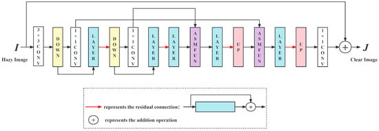
Figure 1.
The overall architecture of Dehaze-UNet.
The downsampling module of Dehaze-UNet is implemented by a convolutional layer with size 2 and stride 2. The upsampling module of Dehaze-UNet is realized by a 1 × 1 convolution layer and a pix-shuffle [37] layer.
3.3. LAYER Module
The designed LAYER module is shown in Figure 2. Each layer is mainly a batch normalization (i.e., BATCHNORM in Figure 2), convolution (i.e., CONV in Figure 2), ReLU activation function (i.e., ReLU in Figure 2), etc. Inspired by the work of batch normalization [31], the proposed LAYER module is a parallel structure, which extracts features separately and finally fuses them in the form of a point product. Through the batch normalization layer, the network can more effectively aggregate the haze features of different hazy images and focus more intently on the haze scene so that the subsequent ASMFUN module can better fit the physical model.
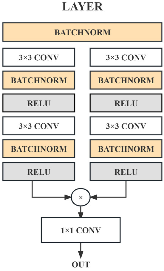
Figure 2.
The structure of the LAYER module.
3.4. ASMFUN Module
The designed ASMFUN module is shown in Figure 3. First, it is a grouped dilated convolution, and the convolution kernel size is 5 × 5. The aim of employing dilated convolution is to enhance the receptive field, and the grouped convolution is to extract the global features of a single channel as much as possible and to make the features of each channel unaffected. Then, after the batch normalization layer, it is activated by the ReLU function, and then there are two parallel structures. This parallel structure is inspired by SKNet [38] and is used to perform high-dimensional abstraction and estimation of and A in ASM. These two parallel structures are composed of an adaptive average pooling layer (i.e., AdaptiveAvgPool2d in Figure 3), 1 × 1 convolution, ReLU activation, and 1 × 1 convolution. The adaptive average pooling layer can effectively extract features, and can change the size of the feature map to a value of 1 × 1 through adaptive parameters; after 1 × 1 convolution, ReLU activation, 1 × 1 convolution, a multichannel 1 × 1 feature map is obtained, which represents the estimated and A with high-dimensional features, respectively. Please note that and A obtained here are not equivalent to the two-dimensional and one-dimensional A in the standard ASM but an abstract result from a higher-dimensional perspective, and then the feature map of the output result is obtained through ASM. The ASM here is not the end-to-end addition of the ASM in most other dehazing methods to obtain hazy or hazy-free images but is embedded as an intermediate layer of the network to operate on the intermediate feature map. This is to allow the network to better understand the formation and removal of haze during the training process. This idea is inspired by the related theory of physics-informed machine learning (PIML) [39]. According to ASM (Equation (1)), can be expressed as
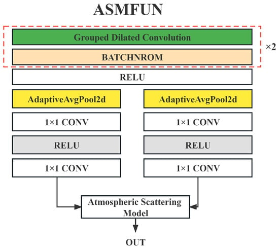
Figure 3.
The structure of ASMFUN module.
However, in the ASMFUN module, ASM is embedded in the intermediate layer to operate on the feature map, not on the final actual output image. Therefore, in order to prevent the situation where the denominator in Equation (3) is 0, a change was made to Equation (3). Assuming that the input of the ASMFUN module is INPUT, and the highly abstract and A obtained by the two parallel structures are and , respectively, the feature map output by the module can be expressed as
The change from the division of Equation (3) to the multiplication in Equation (4) does not mean that the ASM is violated. This is a technical change based on the mechanism of deep learning and experimental observations, which still allows Dehaze-UNet to learn prior knowledge under the constraints of the physical model so that the network can better understand the characteristics of haze. In addition, it is found through experiments that the network trained using the original ASM is difficult to converge, and the loss value appears infinite, while the network trained using the improved Equation (4) is relatively stable.
4. Experiments
4.1. Implementation Details
We performed a lot of comparative experiments on synthetic hazy images and real-world hazy images, including quantitative and qualitative comparative experiments, as well as an ablation study. Our experimental equipment is equipped with 4 NVIDIA GeForce GTX 1080Ti GPUs and uses the Adam optimizer and cosine annealing strategy to train Dehaze-UNet. In order to obtain better model parameters, a pretraining method is adopted; that is, the initial model parameter values are obtained through pretraining with a batch size of 256, a learning rate of 0.002, and a block size of 256 × 256. Formal training is then performed with a batch size of 32, a learning rate of 0.002, and a block size of 512 × 512, where the value of the learning rate is reduced to 0.00002 by a cosine annealing strategy. To verify the performance of Dehaze-UNet, 9 advanced dehazing methods were selected for qualitative and quantitative experimental comparisons. These methods include DCP [2], DehazeNet [9], AODNet [11], GridDehazeNet [16], MSBDN [12], FFANet [17], RefineDNet [18], PSD [19], D4 [20], and DehazeFormer [29]. Among them, DCP [2] is a prior-based method, and the rest are based on deep learning methods. We adopt the well-known PSNR and SSIM indicators [40] for experiments. The higher the scores of these two indicators, the better the recovery performance of the method.
4.1.1. Synthesize Image Dataset
We chose the well-known RESIDE dataset [41], trained on ITS and OTS and then tested on SOTS.
4.1.2. Real-World Image Dataset
For real-world hazy images, the O-Haze [42], NH-Haze [43], and Dense-Haze [44] datasets were chosen. Dehaze-UNet is retrained with the NH-Haze dataset and then evaluated on O-HAZE; similarly, Dehaze-UNet is retrained with the O-Haze dataset and evaluated on NH-Haze and Dense-Haze.
4.2. Experiments on Synthetic Hazy Images
The SOTS dataset from RESIDE [41] was selected for comparative experiments. The SOTS-Indoor is a synthetic indoor hazy image dataset. Two images from this dataset were randomly selected for qualitative comparison experiments. Figure 4 shows the results of clear images restored by different dehazing methods. From Image 1, compared with the ground truth (GT), the image restored by DCP is darker. The color information of the images restored by DehazeNet, AODNet, GridDehazeNet, MSBDN, D4, and other methods is insufficient, and some of the detailed information marked by the red box in Figure 4 is also biased. The image restored by the RefineDNet method has obvious noise, especially the part marked by the red box, and the image restored by the PSD method is obviously brighter. The results restored by the Dehaze-UNet method and the FFANet method are similar and are closest to the GT image. From the PNSR/SSIM index score results of the restored image, the PNSR index score of the image restored by the Dehaze-UNet method is the highest, indicating its excellent performance. The SSIM index score of the Dehaze-UNet method is second only to FFANet, and the difference is only 0.0034, indicating that the performance of the two methods is close. The recovery in Image 2 has a similar situation. From the score, the PSNR index score of the Dehaze-UNet method is second only to FFANet, and the SSIM index score is lower than the FFANet and GridDehazeNet methods. Although the index score restored by Dehaze-UNet did not achieve the highest value, it still shows that Dehaze-UNet is competitive, and it further demonstrates that the FFANet exhibits superior performance on the synthetic dataset.
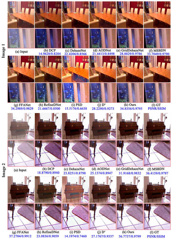
Figure 4.
Comparison of the dehazing effects in the SOTS-Indoor dataset: (a): hazy image, (b–j): the results restored by other advanced methods, (k): the results restored by Dehaze-UNet, (l): the GT image.
The SOTS-Outdoor is a synthetic outdoor hazy image dataset. Two images from this dataset were randomly selected for qualitative comparison experiments. Figure 5 shows the visual results of images restored by different dehazing methods. As can be seen from Image 3 in Figure 5, the image restored by DCP is darker and has severe distortion in the sky area. The image restored by the DehazeNet and AODNet methods is insufficiently protected in the sky area. The images restored by the GridDehazeNet, MSBDN, and D4 methods have chromatic aberrations in the sunlight peripheral part enlarged by the red box. The brightness of the images restored by the FFANet and PSD methods exceeds the GT image. The image restored by the RefineDNet method has severe noise; while the image restored by the Dehaze-UNet is closest to the GT image. From the PNSR/SSIM index results of the restored image, the Dehaze-UNet method has the highest PNSR index, and the SSIM index is second only to GridDehazeNet, with a difference of only 0.0014, which strongly illustrates the advanced performance of Dehaze-UNet. Similarly, from the restored result of Image 4, the restored result of the Dehaze-UNet method is closest to GT in terms of the dehazing effect and the restoration of the color and edge information of the image. Furthermore, the PNSR/SSIM index of the Dehaze-UNet method is the highest, and the PSNR index far exceeds other methods, which illustrates the advanced performance of the Dehaze-UNet.
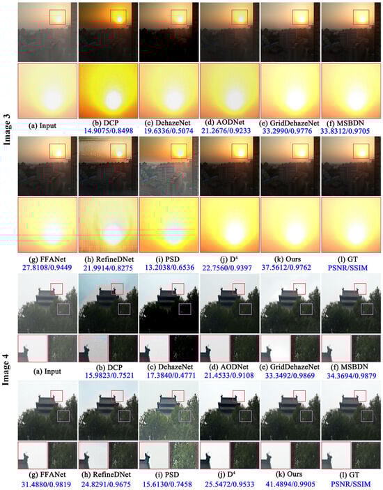
Figure 5.
Comparison of the dehazing effects in the SOTS-Outdoor dataset: (a): hazy image, (b–j): the results restored by other advanced methods, (k): the results restored by Dehaze-UNet, (l): the GT image.
In addition, in order to further compare the performance of various methods, we conducted quantitative experimental comparisons on all images of the SOTS-Indoor and SOTS-Outdoor datasets. The recovery results obtained by different methods were tested on all images of the two datasets, and the average PNSR/SSIM index score was calculated. From Table 1, the SOTS-Indoor dataset with the Dehaze-UNet method obtained the highest PSNR score, while the SSIM score differed from the highest value by about 0.03. For the SOTS-Outdoor dataset, the Dehaze-UNet achieved the highest PNSR score and the second-highest SSIM score. The Dehaze-UNet method achieved the highest PSNR score, which strongly illustrates its superiority. However, the Dehaze-UNet method did not achieve the highest SSIM score. This is because SSIM mainly evaluates based on the structural similarity of images. Since Dehaze-UNet adopts the U-Net structure, the original structural information of the image may be destroyed during the downsampling process. This is also a point that requires further research and improvement in the future.

Table 1.
Quantitative experimental comparison results of synthetic images. Bold numbers indicate the highest indicator score, and underlined numbers indicate the next highest score.
4.3. Experiments on Real-world Scenes
Two images were randomly selected from the O-Haze [42], NH-Haze [43], and Dense-Haze [44] datasets, respectively, for comparison, as shown in Figure 6, Figure 7 and Figure 8. From Figure 6, the results recovered by DCP, AODNet, GridDehazeNet, and RefineDNet are darker, and the results recovered by DehazeNet, MSBDN, FFANet, PSD, and D4 contain obvious residual haze. There is basically no obvious haze in the recovery results of Dehaze-UNet. From the PSNR/SSIM indicators, in the recovery results of Image 5, the Dehaze-UNet method achieved the highest score. For the recovery results of Image 6, the Dehaze-UNet achieved the highest PSNR score, and SSIM was second only to the RefineDNet. This also illustrates the competitive performance of the Dehaze-UNet. However, the color of the result restored by the Dehaze-UNet method is distorted, and the color information cannot be maintained while removing haze. This is also a shortcoming of Dehaze-UNet. Future work will improve this shortcoming.
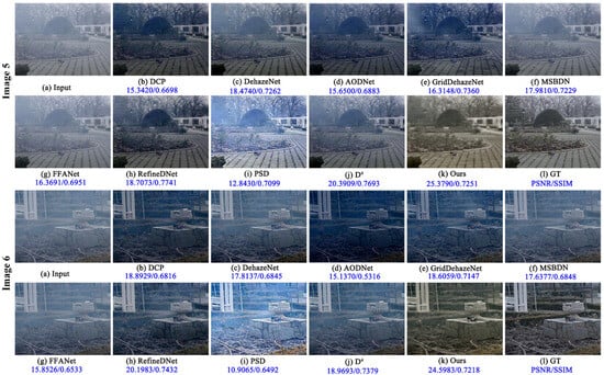
Figure 6.
Comparison of the dehazing effects in the O-Haze dataset: (a): hazy image, (b–j): the results restored by other advanced methods, (k): the results restored by Dehaze-UNet, (l): the GT image.
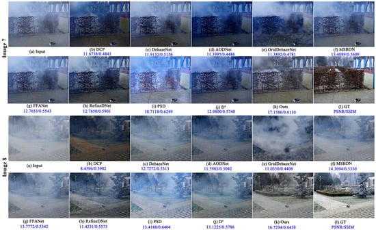
Figure 7.
Comparison of the dehazing effects in the NH-Haze dataset: (a): hazy image, (b–j): the results restored by other advanced methods, (k): the results restored by Dehaze-UNet, (l): the GT image.
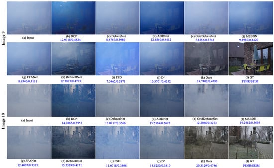
Figure 8.
Comparison of the dehazing effects in the Dense-Haze dataset: (a): hazy image, (b–j): the results restored by other advanced methods, (k): the results restored by Dehaze-UNet, (l): the GT image.
Figure 7 is the experimental comparison result of NH-Haze. As can be seen from Image 7, the results recovered by DCP, AODNet, GridDehazeNet, and RefineDNet are darker. Except for DCP, the remaining methods have very poor dehazing effects, and the recovered images still have a large amount of haze, while the results of the Dehaze-UNet have relatively minimal residual haze. As can be seen from Image 8, the results restored by the DCP and Dehaze-UNet still have the least residual haze, which illustrates the superior performance for outdoor nonuniform hazy images. It also shows that the effectiveness of traditional prior knowledge such as DCP for nonuniform hazy scenes basically exceeds other methods based on deep learning. However, the DCP recovery result is still darker, while the Dehaze-UNet method recovery result is closest to the GT image. It can be seen from the PSNR/SSIM index in the figure that for Image 7, the SSIM score obtained by the Dehaze-UNet is slightly lower than PSD. However, it is obvious that the results of PSD recovery are inferior to the results of the Dehaze-UNet method in terms of color and dehazing ability. This also shows the limitations of the quantitative evaluation index from another perspective; that is, a high PSNR/SSIM index score does not necessarily imply that the visual effect will be equally superior. This is also an issue that requires attention in the field of image dehazing.
In Figure 8, due to the dense haze scene of the Dense-Haze dataset, the recovery results of various advanced dehazing methods are unsatisfactory. However, it can be seen that the recovery result of Dehaze-UNet is still closest to the GT image. From the PSNR/SSIM index in the figure, the index score obtained by the Dehaze-UNet method is the highest, which also verifies the effectiveness of the Dehaze-UNet method in dense haze scenes.
In addition, quantitative experimental comparisons were made on the entire images from the three datasets. The restoration results from different methods were evaluated on all images in these datasets, and the average PSNR/SSIM indicator scores were calculated. The quantitative evaluation results are shown in Table 2. From the PSNR indicator, Dehaze-UNet basically obtained the highest scores and was significantly better than the second-ranked method. Only for the O-Haze dataset, the SSIM result of the Dehaze-UNet method is about 0.03 less than the highest. The above qualitative and quantitative experimental comparisons strongly prove the excellent performance of the Dehaze-UNet method on real scenes.
Table 2.
Quantitative experimental comparison results of the real-world hazy images. Bold numbers indicate the highest indicator score, and underlined numbers indicate the next highest score.
However, Dehaze-UNet also exhibits limitations in real hazy scenes. For example, it does not maintain the color information of the image well while achieving haze removal, such as Image 5 and Image 6. In nonuniform and dense haze scenes, Dehaze-UNet’s dehazing is still not thorough enough, such as in Image 7 and Image 9. This is mainly because there are too few real image samples participating in the training, and the performance of the trained model is not good enough. These shortcomings are a future research direction.
4.4. Parameter and Computational Complexity Analysis
From Table 3, it can be seen that the number of parameters of the Dehaze-UNet model is significantly lower compared with the more famous works since 2019, including GridDehazeNet, MSBDN, FFANet, RefineDNet, PSD, and D4. In addition, the FLOPs of the Dehaze-UNet model are also very small, which are also much lower than GridDehazeNet, MSBDN, FFANet, RefineDNet, PSD, D4, and DehazeFormer-T. This shows that the Dehaze-UNet is a highly lightweight model and is easy to deploy on terminal devices. This is also the key point of our study of this model. Therefore, the proposed method provides a theoretical reference for the lightweight dehazing model.
Table 3.
Comparison of parameters (# Param) and the number of floating-point operations (FLOPs). Where the FLOPs are tested on the image of size 256 × 256.
4.5. Ablation Study
This section mainly studies the impact of Dehaze-UNet’s LAYER module and ASMFUN module on network performance through ablation experiments. In Dehaze-UNet, only the LAYER module, only the ASMFUN module, and both the LAYER and ASMFUN modules were removed to retrain the network and test its performance. Retraining was performed on the ITS dataset and testing on the SOTS-Indoor dataset, respectively. The visual results of the ablation experiment are shown in Figure 9, where the blue text indicates the PSNR/SSIM value. It can be seen from Figure 9 that the image restored without the LAYER and ASMFUN modules has poor recovery of details and is not smooth enough (Figure 9b); the image restored without the LAYER module is smoother (Figure 9c), but the recovery of detail information is still not good; and the image recovered without the ASMFUN module has color distortion (Figure 9d). The result restored by the complete Dehaze-UNet model is closer to the GT image (Figure 9e). The PSNR and SSIM indicator values in the figure also demonstrate the performance of adding these modules.
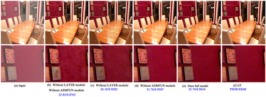
Figure 9.
Visual results of ablation experiments.
The quantitative ablation study results are shown in Table 4. It can be found that adding each module can improve the PSNR and SSIM scores, which illustrates the effectiveness of these two modules.
Table 4.
Ablation study of the network, where w/o means to remove the module.
5. Conclusions and Future Work
This study introduced a lightweight dehazing model, Dehaze-UNet, focusing on its practical application. This model is based on the U-Net structure, which is a pure convolution operation model, and it is designed with a LAYER module and an ASMFUN module. The LAYER module aggregates haze and clear scene characteristics from various hazy images through batch normalization, focusing the network on haze and clear scene features. The ASMFUN module primarily integrates physical models to enable the network to learn prior knowledge during training, enhancing its understanding of haze generation and removal processes and improving overall generalization. Experimental results show that the proposed network model can not only achieve better dehazing effects but also has a small number of model parameters and low computational overhead, making it easy to deploy on terminal devices and improving the practicality of the model.
However, the SSIM index value of the proposed model is not the highest in the experiment, indicating that the model may not preserve the structural information of the image adequately. This is due to the downsampling of the U-Net structure not maintaining enough image structural information. To a certain extent, it is also related to the simple L1 loss function used. Future work should study how to effectively maintain the structural information of the image and try to introduce other loss functions, such as the SSIM loss function, GAN loss function, etc., and appropriately increase the network depth, add convolutional layers, etc., to further improve the model’s performance. Furthermore, the proposed method once again illustrates the necessity of letting the network learn prior knowledge from the fused physical model. In future work, we will try to extend it to video dehazing, addressing dynamic scenes, or exploring domain adaptation for varying atmospheric conditions.
Author Contributions
Writing—original draft preparation, H.Z.; writing—review and editing, Q.L.; supervision, T.T.; experiment, Z.C. All authors have read and agreed to the published version of the manuscript.
Funding
This work was supported by the Anhui University of Technology Young Teachers Research Fund Project (QZ202313), the Key Program of the Natural Science Foundation of the Educational Commission of Anhui Province of China (Grant No. 2022AH050319), and the University Synergy Innovation Program of Anhui Province (GXXT-2023-021).
Data Availability Statement
Data are contained within the article and available online at https://github.com/hocking-cloud/Dehaze-UNet/tree/main.
Conflicts of Interest
The authors declare no conflicts of interest.
References
- Narasimhan, S.G.; Nayar, S.K. Vision and the atmosphere. Int. J. Comput. Vis. 2002, 48, 233–254. [Google Scholar] [CrossRef]
- He, K.; Sun, J.; Tang, X. Single image haze removal using dark channel prior. IEEE Trans. Pattern Anal. Mach. Intell. 2010, 33, 2341–2353. [Google Scholar] [PubMed]
- Yan, Y.; Ren, W.; Guo, Y.; Wang, R.; Cao, X. Image deblurring via extreme channels prior. In Proceedings of the IEEE Conference on Computer Vision and Pattern Recognition 2017, Honolulu, HI, USA, 21–26 July 2017; pp. 4003–4011. [Google Scholar]
- Berman, D.; Avidan, S. Non-local image dehazing. In Proceedings of the IEEE Conference on Computer Vision and Pattern Recognition 2016, Las Vegas, NV, USA, 27–30 June 2016; pp. 1674–1682. [Google Scholar]
- Singh, D.; Kumar, V.; Kaur, M. Single image dehazing using gradient channel prior. Appl. Intell. 2019, 49, 4276–4293. [Google Scholar] [CrossRef]
- Ling, P.; Chen, H.; Tan, X.; Jin, Y.; Chen, E. Single Image Dehazing Using Saturation Line Prior. IEEE Trans. Image Process. 2023, 32, 3238–3253. [Google Scholar] [CrossRef] [PubMed]
- Kumari, A.; Sahoo, S.K. A new fast and efficient dehazing and defogging algorithm for single remote sensing images. Signal Process. 2024, 215, 109289. [Google Scholar] [CrossRef]
- Ajith, A.P.; Vidyamol, K.; Devassy, B.R.; Manju, P. Dark Channel Prior based Single Image Dehazing of Daylight Captures. In Proceedings of the 2023 Advanced Computing and Communication Technologies for High Performance Applications (ACCTHPA), IEEE, Ernakulam, India, 20–21 January 2023; pp. 1–6. [Google Scholar]
- Cai, B.; Xu, X.; Jia, K.; Qing, C.; Tao, D. Dehazenet: An end-to-end system for single image haze removal. IEEE Trans. Image Process. 2016, 25, 5187–5198. [Google Scholar] [CrossRef] [PubMed]
- Ren, W.; Liu, S.; Zhang, H.; Pan, J.; Cao, X.; Yang, M.H. Single image dehazing via multi-scale convolutional neural networks. In Proceedings of the Computer Vision–ECCV 2016: 14th European Conference, Amsterdam, The Netherlands, 11–14 October 2016; Part II 14. Springer: Berlin/Heidelberg, Germany, 2016; pp. 154–169. [Google Scholar]
- Li, B.; Peng, X.; Wang, Z.; Xu, J.; Feng, D. Aod-net: All-in-one dehazing network. In Proceedings of the IEEE International Conference on Computer Vision 2017, Venice, Italy, 22–29 October 2017; pp. 4770–4778. [Google Scholar]
- Dong, H.; Pan, J.; Xiang, L.; Hu, Z.; Zhang, X.; Wang, F.; Yang, M.H. Multi-scale boosted dehazing network with dense feature fusion. In Proceedings of the IEEE/CVF Conference on Computer Vision and Pattern Recognition 2020, Seattle, WA, USA, 13–19 June 2020; pp. 2157–2167. [Google Scholar]
- Wang, C.; Chen, R.; Lu, Y.; Yan, Y.; Wang, H. Recurrent context aggregation network for single image dehazing. IEEE Signal Process. Lett. 2021, 28, 419–423. [Google Scholar] [CrossRef]
- Song, X.; Zhou, D.; Li, W.; Dai, Y.; Shen, Z.; Zhang, L.; Li, H. TUSR-Net: Triple Unfolding Single Image Dehazing With Self-Regularization and Dual Feature to Pixel Attention. IEEE Trans. Image Process. 2023, 32, 1231–1244. [Google Scholar] [CrossRef] [PubMed]
- Yi, W.; Dong, L.; Liu, M.; Hui, M.; Kong, L.; Zhao, Y. Towards Compact Single Image Dehazing via Task-related Contrastive Network. Expert Syst. Appl. 2024, 235, 121130. [Google Scholar] [CrossRef]
- Liu, X.; Ma, Y.; Shi, Z.; Chen, J. Griddehazenet: Attention-based multi-scale network for image dehazing. In Proceedings of the IEEE/CVF International Conference on Computer Vision 2019, Seoul, Republic of Korea, 27 October–2 November 2019; pp. 7314–7323. [Google Scholar]
- Qin, X.; Wang, Z.; Bai, Y.; Xie, X.; Jia, H. FFA-Net: Feature fusion attention network for single image dehazing. In Proceedings of the AAAI Conference on Artificial Intelligence 2020, New York, NY, USA, 7–12 February 2020; Volume 34, pp. 11908–11915. [Google Scholar]
- Zhao, S.; Zhang, L.; Shen, Y.; Zhou, Y. RefineDNet: A weakly supervised refinement framework for single image dehazing. IEEE Trans. Image Process. 2021, 30, 3391–3404. [Google Scholar] [CrossRef]
- Chen, Z.; Wang, Y.; Yang, Y.; Liu, D. PSD: Principled synthetic-to-real dehazing guided by physical priors. In Proceedings of the IEEE/CVF Conference on Computer Vision and Pattern Recognition 2021, Nashville, TN, USA, 20–25 June 2021; pp. 7180–7189. [Google Scholar]
- Yang, Y.; Wang, C.; Liu, R.; Zhang, L.; Guo, X.; Tao, D. Self-augmented unpaired image dehazing via density and depth decomposition. In Proceedings of the IEEE/CVF Conference on Computer Vision and Pattern Recognition 2022, New Orleans, LA, USA, 18–24 June 2022; pp. 2037–2046. [Google Scholar]
- Zhang, K.; Li, Y. Single image dehazing via semi-supervised domain translation and architecture search. IEEE Signal Process. Lett. 2021, 28, 2127–2131. [Google Scholar] [CrossRef]
- Hong, M.; Xie, Y.; Li, C.; Qu, Y. Distilling image dehazing with heterogeneous task imitation. In Proceedings of the IEEE/CVF Conference on Computer Vision and Pattern Recognition 2020, Seattle, WA, USA, 13–19 June 2020; pp. 3462–3471. [Google Scholar]
- Kim, G.; Kwon, J. Self-Parameter Distillation Dehazing. IEEE Trans. Image Process. 2022, 32, 631–642. [Google Scholar] [CrossRef]
- Wu, H.; Qu, Y.; Lin, S.; Zhou, J.; Qiao, R.; Zhang, Z.; Xie, Y.; Ma, L. Contrastive learning for compact single image dehazing. In Proceedings of the IEEE/CVF Conference on Computer Vision and Pattern Recognition 2021, Nashville, TN, USA, 20–25 June 2021; pp. 10551–10560. [Google Scholar]
- Zheng, Y.; Zhan, J.; He, S.; Dong, J.; Du, Y. Curricular contrastive regularization for physics-aware single image dehazing. In Proceedings of the IEEE/CVF Conference on Computer Vision and Pattern Recognition 2023, Vancouver, BC, Canada, 17–24 June 2023; pp. 5785–5794. [Google Scholar]
- Valanarasu, J.M.J.; Yasarla, R.; Patel, V.M. Transweather: Transformer-based restoration of images degraded by adverse weather conditions. In Proceedings of the IEEE/CVF Conference on Computer Vision and Pattern Recognition 2022, New Orleans, LA, USA, 18–24 June 2022; pp. 2353–2363. [Google Scholar]
- Guo, C.L.; Yan, Q.; Anwar, S.; Cong, R.; Ren, W.; Li, C. Image dehazing transformer with transmission-aware 3d position embedding. In Proceedings of the IEEE/CVF Conference on Computer Vision and Pattern Recognition 2022, New Orleans, LA, USA, 18–24 June 2022; pp. 5812–5820. [Google Scholar]
- Zhou, H.; Chen, Z.; Liu, Y.; Sheng, Y.; Ren, W.; Xiong, H. Physical-priors-guided DehazeFormer. Knowl.-Based Syst. 2023, 266, 110410. [Google Scholar] [CrossRef]
- Song, Y.; He, Z.; Qian, H.; Du, X. Vision transformers for single image dehazing. IEEE Trans. Image Process. 2023, 32, 1927–1941. [Google Scholar] [CrossRef]
- Ronneberger, O.; Fischer, P.; Brox, T. U-net: Convolutional networks for biomedical image segmentation. In Proceedings of the Medical Image Computing and Computer-Assisted Intervention–MICCAI 2015: 18th International Conference, Munich, Germany, 5–9 October 2015; Proceedings, Part III 18. Springer: Berlin/Heidelberg, Germany, 2015; pp. 234–241. [Google Scholar]
- Huang, L.; Zhou, Y.; Wang, T.; Luo, J.; Liu, X. Delving into the estimation shift of batch normalization in a network. In Proceedings of the IEEE/CVF Conference on Computer Vision and Pattern Recognition 2022, New Orleans, LA, USA, 18–24 June 2022; pp. 763–772. [Google Scholar]
- Zhu, Q.; Mai, J.; Shao, L. A fast single image haze removal algorithm using color attenuation prior. IEEE Trans. Image Process. 2015, 24, 3522–3533. [Google Scholar]
- Berman, D.; Treibitz, T.; Avidan, S. Single image dehazing using haze-lines. IEEE Trans. Pattern Anal. Mach. Intell. 2018, 42, 720–734. [Google Scholar] [CrossRef] [PubMed]
- Li, C.; Yuan, C.; Pan, H.; Yang, Y.; Wang, Z.; Zhou, H.; Xiong, H. Single-Image Dehazing Based on Improved Bright Channel Prior and Dark Channel Prior. Electronics 2023, 12, 299. [Google Scholar] [CrossRef]
- Yu, H.; Zheng, N.; Zhou, M.; Huang, J.; Xiao, Z.; Zhao, F. Frequency and spatial dual guidance for image dehazing. In Proceedings of the European Conference on Computer Vision, Tel Aviv, Israel, 23–27 October 2022; Springer: Berlin/Heidelberg, Germany, 2022; pp. 181–198. [Google Scholar]
- Li, B.; Gou, Y.; Gu, S.; Liu, J.Z.; Zhou, J.T.; Peng, X. You only look yourself: Unsupervised and untrained single image dehazing neural network. Int. J. Comput. Vis. 2021, 129, 1754–1767. [Google Scholar] [CrossRef]
- Wang, D.; Zhuang, L.; Gao, L.; Sun, X.; Huang, M.; Plaza, A. PDBSNet: Pixel-shuffle Down-sampling Blind-Spot Reconstruction Network for Hyperspectral Anomaly Detection. IEEE Trans. Geosci. Remote Sens. 2023, 61, 5511914. [Google Scholar] [CrossRef]
- Li, X.; Wang, W.; Hu, X.; Yang, J. Selective kernel networks. In Proceedings of the IEEE/CVF Conference on Computer Vision and Pattern Recognition 2019, Long Beach, CA, USA, 15–20 June 2020; pp. 510–519. [Google Scholar]
- Meng, C.; Seo, S.; Cao, D.; Griesemer, S.; Liu, Y. When physics meets machine learning: A survey of physics-informed machine learning. arXiv 2022, arXiv:2203.16797. [Google Scholar]
- Wang, Z.; Bovik, A.C.; Sheikh, H.R.; Simoncelli, E.P. Image quality assessment: From error visibility to structural similarity. IEEE Trans. Image Process. 2004, 13, 600–612. [Google Scholar] [CrossRef] [PubMed]
- Li, B.; Ren, W.; Fu, D.; Tao, D.; Feng, D.; Zeng, W.; Wang, Z. Benchmarking single-image dehazing and beyond. IEEE Trans. Image Process. 2018, 28, 492–505. [Google Scholar] [CrossRef] [PubMed]
- Ancuti, C.O.; Ancuti, C.; Timofte, R.; De Vleeschouwer, C. O-haze: A dehazing benchmark with real hazy and haze-free outdoor images. In Proceedings of the IEEE Conference on Computer Vision and Pattern Recognition Workshops 2018, Salt Lake City, UT, USA, 18–23 June 2018; pp. 754–762. [Google Scholar]
- Ancuti, C.O.; Ancuti, C.; Timofte, R. NH-HAZE: An image dehazing benchmark with non-homogeneous hazy and haze-free images. In Proceedings of the IEEE/CVF Conference on Computer Vision and Pattern Recognition Workshops 2020, Seattle, WA, USA, 14–19 June 2020; pp. 444–445. [Google Scholar]
- Ancuti, C.O.; Ancuti, C.; Sbert, M.; Timofte, R. Dense-haze: A benchmark for image dehazing with dense-haze and haze-free images. In Proceedings of the 2019 IEEE International Conference on Image Processing (ICIP), Taipei, Taiwan, 22–25 September 2019; pp. 1014–1018. [Google Scholar]
Disclaimer/Publisher’s Note: The statements, opinions and data contained in all publications are solely those of the individual author(s) and contributor(s) and not of MDPI and/or the editor(s). MDPI and/or the editor(s) disclaim responsibility for any injury to people or property resulting from any ideas, methods, instructions or products referred to in the content. |
© 2024 by the authors. Licensee MDPI, Basel, Switzerland. This article is an open access article distributed under the terms and conditions of the Creative Commons Attribution (CC BY) license (https://creativecommons.org/licenses/by/4.0/).