Research on a Personalized Decision Control Algorithm for Autonomous Vehicles Based on the Reinforcement Learning from Human Feedback Strategy

Abstract

To address the shortcomings of previous autonomous decision models, which often overlook the personalized features of users, this paper proposes a personalized decision control algorithm for autonomous vehicles based on RLHF (reinforcement learning from human feedback). The algorithm combines two reinforcement learning approaches, DDPG (Deep Deterministic Policy Gradient) and PPO (proximal policy optimization), and divides the control scheme into three phases including pre-training, human evaluation, and parameter optimization. During the pre-training phase, an agent is trained using the DDPG algorithm. In the human evaluation phase, different trajectories generated by the DDPG-trained agent are scored by individuals with different styles, and the respective reward models are trained based on the trajectories. In the parameter optimization phase, the network parameters are updated using the PPO algorithm and the reward values given by the reward model to achieve personalized autonomous vehicle control. To validate the control algorithm designed in this paper, a simulation scenario was built using CARLA_0.9.13 software. The results demonstrate that the proposed algorithm can provide personalized decision control solutions for different styles of people, satisfying human needs while ensuring safety.

1. Introduction

Autonomous technology can ease traffic congestion, improve road traffic safety, and reduce greenhouse gas emissions, so it has become a hot research topic in recent years. At the present stage, autonomous technology mainly follows fixed rules and procedures to control vehicles, i.e., through radar, camera, positioning systems, and other sensors that collect sensory data in the actual driving scene, combined with the rules of vehicle driving in the real traffic scene to make driving decisions [1]. This control method ignores the personalized characteristics of the driverless user and cannot meet the personalized needs of the user. Autonomous technology based on the personalized characteristics of driving users can make autonomous decisions and control for different driving styles, driving habits, and road conditions, which can satisfy different people’s preferences and needs for factors such as safety, comfort, and stability, and then provide a more accurate and high-quality user experience [2,3,4,5]. Therefore, personalized decision control for autonomous vehicles is necessary for future development, which has important social significance and research value.

At present, the personalized decision control of automatic vehicles is mainly studied from the following three aspects. First, through the study of the driver’s driving intention by reproducing a driver’s driving decision so as to realize personalized driving. Gindele [6] studied the driver’s driving process and used a hierarchical dynamic Bayesian model to model and reproduce the driver’s decision-making process. Chen [7] collected vehicle motion trajectories using visual sensors, modeled and reproduced the personalized decision-making process of different drivers using sparse representations, and validated the method using four different datasets. Their results showed that the accuracy of the method for classifying and recognizing driving behaviors was significantly higher than that of traditional methods. Yang [8] studied the characteristics of driver following behavior, established a Gaussian mixture model, proposed a driving reference trajectory based on personalized driving, and realized the planning and control of vehicle state dynamics under a complex dynamic environment by designing a quadratic planning optimal controller. Second, some studies have directly integrated the driver model with the control module to achieve personalized driving. Abdul [9] proposed the use of a cerebellar model controller to build a personalized driver’s driving behavior model, which enabled the modeling of different driving behavioral characteristics. Yan [10] established an adaptive cruise control strategy that mimicked a driver’s driving characteristics by analyzing the driver’s driving data. Wang [11] used Gaussian mixture models and hidden Markov models to learn from driving data to obtain a personalized driver model, which was used for vehicle motion trajectory prediction, and then established a personalized lane departure warning strategy. Li [12] established a data-driven personalized vehicle trajectory planning method based on recurrent neural networks with actual driving data. In the third aspect, based on the assisted driving system, lane changing and following during personalized automatic driving were studied. Ramyar [13], Zhu [14], and Huang [15] combined the assisted driving system, considered drivers’ personalized driving behaviors, and designed a control system for lane-changing scenarios in highway environments, which improved driving comfort and ensured driving safety. Zhu [16] used personalized following driving as a research object and guided the learning process of the DDPG following strategy by setting the objective function of consistency evaluation with driving data. The method obtained an anthropomorphic longitudinal following model through continuous trial-and-error interaction with the environment model. Wang [17] improved the DDPG algorithm in order to provide personalized driving services in line with driving habits, added a linear transformation process to the output of the algorithm, and designed a driving decision system for the vehicle so that the vehicle could learn different styles of personalized driving strategies. The results showed that the algorithm enabled the vehicle to maintain a higher level of lateral control than a general driver, and the lane offset, i.e., the extent to which a vehicle’s center of mass is offset from the centerline of the lane, decreased by 73.0%.

The aforementioned research on personalized decision control for autonomous vehicles mainly focuses on the identification, modeling, and analysis of driving styles, mostly based on assisted driving systems. A large number of constraints have been added to the research, and the dimensions of the state space and action space considered are lower. These are only applicable to the personalized decision control of autonomous vehicles in specific scenarios, such as following a car and changing lane scenarios, and do not consider multi-dimensional and multi-driving environment scenarios. Therefore, it is impossible to realize the personalized decision control of autonomous vehicles in the real sense and impossible to meet the requirements of different people for safety, comfort, and stability.

Aiming at the current problem of low dimensionality in the state space and the action space considered in personalized decision control for autonomous vehicles and poor adaptability, this paper innovatively introduces human feedback and designs a personalized decision control algorithm for autonomous vehicles based on the RLHF strategy. This strategy combines two reinforcement learning algorithms, namely, DDPG and PPO, and trains agents in three phases, including pre-training, human evaluation, and parameter optimization, so that the algorithm can be adapted to different styles of people and different scenarios. Then, simulation scenarios were built to train the designed control algorithms based on different driving styles, and finally, the effectiveness of the algorithms designed in this paper was verified through typical scenario simulations. The algorithm proposed in this paper can provide personalized decision control schemes for people with different driving styles and can adapt to different driving environments to maximize the satisfaction of human needs while ensuring safety, thus providing a reference for the personalized control of unmanned vehicles.

The main contributions of this paper lie firstly in proposing a personalized decision-making framework for automated driving that incorporates policy transfer and human–computer interactions. The framework utilizes knowledge learned from large-scale driving data to pre-train a generic policy, employs active learning to efficiently query human preferences for the most informative driving trajectories, and finally, finely tunes the pre-trained policy according to the individual’s driving style so as to adapt rapidly in the presence of limited personalized driving data. Secondly, the proposed RLHF approach offers higher interpretability and transparency as the model’s reward signals are derived from human-preferred trajectories rather than human-annotated labels, which reduces the influence of human factors on the learning outcome. This is a promising alternative to traditional approaches relying on predefined reward functions and can help to overcome the challenge of designing reward functions that accurately reflect the complexity of real-world situations.

2. Design of a Personalized Control Strategy for Autonomous Vehicles Based on Human Feedback

2.1. General Framework Design of a Personalized Control Strategy for Autonomous Vehicles Based on Human Feedback

The overall framework of the human feedback-based personalized control strategy algorithm for autonomous vehicles designed in this paper is shown in Figure 1, which is divided into three main phases. The first phase is a pre-training phase, where the DDPG algorithm is used to train the autonomous vehicles until the agent can complete the passage task efficiently. The second phase is the human evaluation phase, where the agent is tested on random roads and environments and its trajectories are recorded. These trajectories are presented to the human for evaluation, with a pair of trajectories taken for each evaluation to determine the differences between them. By repeatedly evaluating multiple sets of trajectories, enough data are thus obtained to train the reward model. The third phase is the parameter optimization phase, where the current reward model is used to score the actions and the PPO algorithm is used to fine-tune the parameters of the agent trained in the first phase. Each phase is described in detail next.

Figure 1. General framework diagram of the personalized control strategy for autonomous vehicles based on human feedback.

2.2. Principle of the Algorithm Used in the Pre-Training Phase

The pre-training phase uses the DDPG algorithm to train the autonomous vehicles until the agent can efficiently perform the passage task. The goal of this phase is to train an agent with basic driving capabilities.

The DDPG algorithm is a deep neural network-based reinforcement learning algorithm that can be used to solve continuous action space problems. In the continuous action space, an agent can take any real-valued action. It is based on Actor–Critic, using the policy network $u\left(\mathrm{s};\mathsf{\theta }\right)$ for decision output and the value network $\mathrm{Q}\left(\mathrm{s},a;\mathsf{\omega }\right)$ for scoring the decisions performed by the policy network. This in turn guides the policy network for improvement, as well as using experience replay and target networks to stabilize the training process [18,19].

In policy network training, DDPG uses deterministic strategy gradient DPG to make ${\nabla }_{\mathsf{\theta }}\mathrm{J}\left(\mathsf{\theta }\right)$ unbiased estimations:

$${\nabla }_{\mathsf{\theta }}\mathrm{J}\left(\mathsf{\theta }\right)={\nabla }_{\mathsf{\theta }}u\left(\mathrm{s};\mathsf{\theta }\right)·{\nabla }_{\mathrm{w}}\mathrm{Q}\left(\mathrm{s},a;\mathsf{\omega }\right)$$

(1)

Thus, the updated algorithm is obtained. Then, a state from the experience replay cache is randomly selected each time, denoted as $s_j$, $a_j=\mu \left(s_j;\theta \right)$ is calculated, and $\mathsf{\theta }$ is updated using the gradient rise formula:

$$\mathsf{\theta }\leftarrow \mathsf{\theta }+\mathsf{\beta }·{\nabla }_{\mathsf{\theta }}u\left({\mathrm{s}}_{\mathrm{j}};\mathsf{\theta }\right)·{\nabla }_{\mathsf{\omega }}\mathrm{Q}\left({\mathrm{s}}_{\mathrm{j}},a_{\mathrm{j}};\mathsf{\omega }\right)$$

(2)

where $\mathsf{\beta }$ is the learning rate, which generally needs to be adjusted manually.

The TD algorithm is used to make the prediction of the value network closer to the TD target and the predicted value of the target network closer to the real value function, that is

$$\mathrm{Q}\left(\mathrm{s},a;\mathsf{\omega }\right)\cong {\mathrm{Q}}_{\mathsf{\pi }}\left(\mathrm{s},a\right)$$

(3)

The gradient is expressed as:

$${\nabla }_{\mathsf{\omega }}L\left(\mathsf{\omega }\right)=\left[\mathrm{Q}\left(s,a;\mathsf{\omega }\right)-r-\mathrm{Q}\left(s^{\prime },a^{\prime };\mathsf{\omega }\right)\right]·{\nabla }_{\omega }\mathrm{Q}\left(s,a;\mathsf{\omega }\right)$$

(4)

The updating formula of the value network is as follows:

$$\mathsf{\omega }\leftarrow \mathsf{\omega }-\mathsf{\alpha }·{\mathsf{\delta }}_{\mathrm{j}}{\nabla }_{\mathsf{\omega }}\mathrm{Q}\left(\mathrm{s},a;\mathsf{\omega }\right)$$

(5)

Using soft-update, the update formula is as follows:

$${{\theta }^{-}}_{new}\leftarrow \tau ·{\theta }_{new}+\left(1-\tau \right){{\theta }^{-}}_{now}$$

(6)

$${{\omega }^{-}}_{new}\leftarrow \tau ·{\omega }_{new}+\left(1-\tau \right){{\omega }^{-}}_{now}$$

(7)

where $\tau$ is a hyperparameter that needs to be adjusted manually.

The DDPG algorithm is shown in Algorithm 1.

Algorithm 1 DDPG algorithm training process
1	Begin
2	Initialization
3	$\mathrm{Random}\mathrm{initialization}\mathrm{of}\mathrm{the}\mathrm{Critic}\mathrm{network}Q\left(s,a;\mathsf{\omega }\right)$ $\mathrm{and}\mathrm{Actor}\mathrm{network}u\left(s;\theta \right)$
4	$\mathrm{Initialize}\mathrm{the}\mathrm{target}\mathrm{network}{\mathsf{\omega }}^{-}\leftarrow \omega$$,{\theta }^{-}\leftarrow \theta$
5	Initialize replay buffer M
6	For episode = 1 to T1, do
7	$\hspace{1em}\mathrm{Initialize}\mathrm{CARLA}\mathrm{environment}\mathrm{and}\mathrm{get}\mathrm{initial}\mathrm{state}{S}_0$
8	For t = 1 to T2, do
9	$\mathrm{According}\mathrm{to}\mathrm{the}\mathrm{noise},\mathrm{current}\mathrm{state}{S}_t$$,\mathrm{the}\mathrm{agent}\mathrm{selects}\mathrm{the}\mathrm{action}{a}_t$
10	$\mathrm{Execute}\mathrm{the}\mathrm{action}\mathrm{to}\mathrm{obtain}\mathrm{the}\mathrm{current}\mathrm{return}{r}_t$ $\mathrm{and}\mathrm{the}\mathrm{next}\mathrm{state}{S}_{t+1}$
11	$\mathrm{Store}\mathrm{the}\mathrm{empirical}\mathrm{samples}\left(s_t,a_t,r_t,s_{t+1}\right)$ to M
12	Calculate the sampling probability according to TD error and rank it in M
13	If the number of stores in M reaches N:
14	$\mathrm{Sample}\mathrm{from}M\mathrm{according}\mathrm{to}\mathrm{the}\mathrm{size}\mathrm{of}\mathrm{the}\mathrm{sampling}\mathrm{probability}\mathrm{mini}\text{-}\mathrm{batch}\left(s_i,a_i,r_i,s_{i+1}\right)$
15	$\hspace{1em}\hspace{1em}\hspace{1em}\hspace{1em}\hspace{1em}\hspace{1em}\hspace{1em}\hspace{1em}\hspace{1em}\hspace{1em}\hspace{1em}\hspace{1em}\hspace{1em}\hspace{1em}\mathrm{Set}{y}_i=r_i+\gamma {\mathrm{Q}}^{\prime }{(\mathrm{s}}_{i+1},u^{\prime }{(\mathrm{s}}_{i+1}\left|{\theta }^{u^{\prime }}\left|{\theta }^{Q^{\prime }}\right.\right.)$
16	$\hspace{1em}\hspace{1em}\hspace{1em}\mathrm{Update}\mathrm{Critic}\mathrm{network}\mathrm{by}\mathrm{minimizing}\mathrm{losses}L=\frac{1}{N}{\sum }_i{\left(y_i-Q\left(s_i,a_i∣\mathsf{\theta }\right)\right)}^2$
17	Updating Actor networks by stochastic gradient descent:
18	${\left.{\left.{\nabla }_{{\mathsf{\theta }}^u}J\approx \frac{1}{N}{\displaystyle \sum _i}{\nabla }_{a}Q\left(s,a∣\mathsf{\theta }\right)\right|}_{s=s_i,a=u\left(s_i\right)}{\nabla }_{{\mathsf{\theta }}^u}u\left(s∣\mathsf{\omega }\right)\right|}_{s_i}$
19	Updated $\mathsf{\theta }$ using the gradient rise formula, where $\mathsf{\beta }$ is the learning rate, which generally needs to be adjusted manually.            $\mathsf{\theta }\leftarrow \mathsf{\theta }+\mathsf{\beta }·{\nabla }_{\mathsf{\theta }}u\left({\mathrm{s}}_{\mathrm{j}};\mathsf{\theta }\right)·{\nabla }_{\mathsf{\omega }}\mathrm{Q}\left({\mathrm{s}}_{\mathrm{j}},a_{\mathrm{j}};\mathsf{\omega }\right)$
20	The gradient is expressed as:             ${\nabla }_{\mathsf{\omega }}L\left(\mathsf{\omega }\right)=\left[Q\left(s,a;\mathsf{\omega }\right)-r-Q\left(s^{\prime },a^{\prime };\mathsf{\omega }\right)\right]·{\nabla }_{\omega }Q\left(s,a;\mathsf{\omega }\right)$
21	The updating formula of the value network is as follows:               $\mathsf{\omega }\leftarrow \mathsf{\omega }-\mathsf{\alpha }·{\mathsf{\delta }}_{\mathrm{j}}{\nabla }_{\mathsf{\omega }}\mathrm{Q}\left(\mathrm{s},a;\mathsf{\omega }\right)$
22	$\hspace{1em}\hspace{1em}\hspace{1em}\mathrm{Update}\mathrm{the}\mathrm{target}\mathrm{network},\mathrm{where}\tau \in (0,1)$, is a hyperparameter that needs to be manually adjusted               ${{\theta }^{-}}_{new}\leftarrow \tau ·{\theta }_{new}+\left(1-\tau \right){{\theta }^{-}}_{now}$               ${{\omega }^{-}}_{new}\leftarrow \tau ·{\omega }_{new}+\left(1-\tau \right){{\omega }^{-}}_{now}$
23	End If
24	$s_t{=s}_{t+1}$
25	End For
26	End For
27	End

2.3. Principle of the Algorithm Used in the Human Evaluation Phase

The human evaluation phase uses the RLHF algorithm to train the agent so as to train a reward model with a similar style to humans. The reward model can either train the policy neural network from scratch based on preference data or fine-tune it based on the pre-trained policy neural network [20]. The goal of this phase is to train reward models that have a similar style to humans through human feedback.

The RLHF algorithm introduces human feedback in reinforcement learning to guide the agent to make updates so that the agent can learn complex tasks and make decisions that are more in line with human behavior; the principle of the algorithm is shown in Figure 2. Here, the reinforcement learning strategy is $\pi \left(a|s\right)$, which is the mapping from the network state to the action, and the reward model is denoted by $\tilde{r}\left(r|s,a\right)$, which is the mapping from the state and action to the reward [21]. The iterative process of RLHF is divided into three main steps as follows: First, the policy π will interact with the environment to generate a series of trajectories $\left\{{\tau }^1,{\tau }^2,\cdots ,{\tau }^i\right\}$, where ${\tau }^i=\left(\left(o_1^i,a_1^i\right),\cdots ,\left(o_{k-1}^i,a_{k-1}^i\right)\right)$; each trajectory is composed of multiple groups of state–action pairs. The parameter update formula for the strategy π uses a traditional reinforcement learning algorithm with the aim of maximizing the sum of the reward values $r_t=\tilde{r}\left(r|s,a\right)$ predicted by the reward model. In the second step, a pair of trajectories {${\sigma }^1,{\sigma }^2$} is randomly selected from the above trajectories and sent to humans for comparison, which is then recorded in a triple $\left({\sigma }^1,{\sigma }^2,\mu \right)$, where $\mu \in \left\{\left(\mathrm{0,1}\right),\left(\mathrm{1,0}\right),\left(\mathrm{0.5,0.5}\right)\right\}$, which can indicate the trajectory that is more biased by humans. In the third step, the parameters of the reward model are optimized by supervised learning. The training of the reward model requires the use of the triad from the second step, where P is the reward model predictor and ${\sigma }^1>{\sigma }^2$ indicates that trajectory 1 is better than trajectory 2. The formula is expressed as follow.

$$\mathrm{P}\left[{\mathsf{\sigma }}^1>{\mathsf{\sigma }}^2\right]=\frac{\mathrm{e}\mathrm{x}\mathrm{p}{\sum }_t\tilde{r}\left({\mathrm{s}}_{\mathrm{t}}^1,{\mathrm{a}}_{\mathrm{t}}^1;\mathsf{\theta }\right)}{\mathrm{e}\mathrm{x}\mathrm{p}{\sum }_t\tilde{r}\left({\mathrm{s}}_{\mathrm{t}}^1,{\mathrm{a}}_{\mathrm{t}}^1;\mathsf{\theta }\right)+\mathrm{e}\mathrm{x}\mathrm{p}{\sum }_t\tilde{r}\left({\mathrm{s}}_{\mathrm{t}}^2,{\mathrm{a}}_{\mathrm{t}}^2;\mathsf{\theta }\right)}$$

(8)

Figure 2. RLHF algorithm.

The loss function of the reward model is as follows:

$${\mathcal{L}}^{\mathrm{R}\mathrm{e}\mathrm{w}\mathrm{a}\mathrm{r}\mathrm{d}}=-{\mathbb{E}}_{\left({\mathsf{\sigma }}^1,{\mathsf{\sigma }}^2,\mathsf{\mu }\right)\sim \mathcal{D}}\left[\mathsf{\mu }\left(0\right)\mathrm{l}\mathrm{o}\mathrm{g}\mathrm{P}\left[{\mathsf{\sigma }}^1>{\mathsf{\sigma }}^2\right]+\mathsf{\mu }\left(1\right)\mathrm{l}\mathrm{o}\mathrm{g}\mathrm{P}\left[{\mathsf{\sigma }}^2>{\mathsf{\sigma }}^1\right]\right]$$

(9)

Once the loss is obtained, the gradient can be calculated, and then the strategy can be optimized.

The reward model, which is continuously trained and updated by human feedback, can replace the traditional reward function and be trained by accessing the normal reinforcement learning algorithm to evaluate the decisions of the agent. Considering that the reward function can change dramatically during the training process, the on-policy algorithm is generally used to circumvent the instability in training. The reward model training algorithm is shown in Algorithm 2.

Algorithm 2 The reward model training algorithm
1	Begin
2	$\mathrm{Initialize}\mathrm{the}\mathrm{reward}\mathrm{model}\mathrm{network}\tilde{r}\left(s_t,a_t;\theta \right)$ $\mathrm{and}\mathrm{trajectory}\mathrm{length}\mathrm{“}\mathit{length}\text{”}$
3	For Epochs = 1 to T, do:
4	$\hspace{1em}\mathrm{Draw}\mathrm{the}\mathrm{triplet}\left({\sigma }^1,{\sigma }^2,\mu \right)$, let t = 0
5	While True:
5	If t ! = length:
6	$\hspace{1em}\hspace{1em}\hspace{1em}\mathrm{Use}\mathrm{the}\mathrm{reward}\mathrm{model}\mathrm{to}\mathrm{score}\mathrm{the}\mathrm{action}\mathrm{of}\mathrm{the}\mathrm{first}\mathrm{trajectory}{r}_{1,t}=\tilde{r}\left({\mathrm{s}}_{\mathrm{t}}^1,{\mathrm{a}}_{\mathrm{t}}^1;\mathsf{\theta }\right)$
7	$\hspace{1em}\hspace{1em}\hspace{1em}\mathrm{Use}\mathrm{the}\mathrm{reward}\mathrm{model}\mathrm{to}\mathrm{score}\mathrm{the}\mathrm{action}\mathrm{for}\mathrm{the}\sec \mathrm{ond}\mathrm{trajectory}{r}_{2,t}=\tilde{r}\left({\mathrm{s}}_{\mathrm{t}}^2,{\mathrm{a}}_{\mathrm{t}}^2;\mathsf{\theta }\right)$
8	$t=t+1$
9	else:      $\mathrm{Define}\mathrm{the}\mathrm{reward}\mathrm{model}\mathrm{predictor},{\sigma }^1>{\sigma }^2$ indicates that trajectory 1 is better than trajectory 2:
10	$\mathrm{P}\left[{\mathsf{\sigma }}^1>{\mathsf{\sigma }}^2\right]=\frac{\mathrm{e}\mathrm{x}\mathrm{p}{\sum }_t\tilde{r}\left({\mathrm{s}}_{\mathrm{t}}^1,{\mathrm{a}}_{\mathrm{t}}^1;\mathsf{\theta }\right)}{\mathrm{e}\mathrm{x}\mathrm{p}{\sum }_t\tilde{r}\left({\mathrm{s}}_{\mathrm{t}}^1,{\mathrm{a}}_{\mathrm{t}}^1;\mathsf{\theta }\right)+\mathrm{e}\mathrm{x}\mathrm{p}{\sum }_t\tilde{r}\left({\mathrm{s}}_{\mathrm{t}}^2,{\mathrm{a}}_{\mathrm{t}}^2;\mathsf{\theta }\right)}$
11	Find the loss function:
12	$\hspace{1em}\hspace{1em}\hspace{1em}\hspace{1em}\hspace{1em}{\mathcal{L}}^{Reward}=-{\mathbb{E}}_{\left({\sigma }^1,{\sigma }^2,\mu \right)\sim \mathcal{D}}\left[\mu \left(0\right)logP\left[{\sigma }^1>{\sigma }^2\right]+\mu \left(1\right)logP\left[{\sigma }^2>{\sigma }^1\right]\right]$
13	$\hspace{1em}\hspace{1em}\hspace{1em}\mathrm{Update}\mathrm{the}\mathrm{network}\mathrm{by}\mathrm{gradient}\mathrm{descent}{\nabla }_{\theta }{\mathcal{L}}^{\mathcal{R}\mathcal{w}\mathcal{r}}$
14	break
15	End For
16	End

2.4. Principle of the Algorithm Used in the Parameter Optimization Phase

The parameter optimization phase scores the actions using the reward model and also updates the parameters of the agent trained in the first phase using the PPO algorithm. The goal of this phase is to further optimize the control strategy and to achieve personalized autonomous vehicle control.

The PPO algorithm is based on the Actor–Critic framework. The high efficiency of this algorithm is due to the fact that it uses a proximal policy-based optimization approach, which does not require second-order approximation or KL scattering constraints and is relatively easy to implement and tune [22,23].

PPO transforms the original optimization term and constraint combination in the confidence domain policy optimization algorithm TRPO into a truncated optimization objective without constraints:

$$E_t\left[\min \left(\frac{{\mathsf{\pi }}_{\mathsf{\theta }}\left(a_t∣s_t\right)}{{\mathsf{\pi }}_{{\mathsf{\theta }}_k}\left(a_t∣s_t\right)}{A}^{{\mathsf{\theta }}_k}\left(s_t,a_t\right),clip\left(\frac{{\mathsf{\pi }}_{\mathsf{\theta }}\left(a_t∣s_t\right)}{{\mathsf{\pi }}_{{\mathsf{\theta }}_k}\left(a_t∣s_t\right)},1-\mathsf{ϵ},1+\mathsf{ϵ}\right)A^{{\mathsf{\theta }}_k}\left(s_t,a_t\right)\right)\right]$$

(10)

Specifically, when the expected returns are good, the PPO algorithm remains cautious and chooses to use the truncation value when $\mathrm{r}\left(\mathsf{\theta }\right)>1+\mathsf{ϵ}$, avoiding aggressive optimization behavior. When the expected returns are poor, the PPO algorithm remains sufficiently punitive and chooses to use the truncation value when $\mathrm{r}\left(\mathsf{\theta }\right)<1-\mathsf{ϵ}$.

The PPO algorithm is shown in Algorithm 3.

Algorithm 3 PPO algorithm process
1	Begin
2	Initialization:
3	$\mathrm{Initialize}\mathrm{the}\mathrm{policy}\mathrm{network}\mathrm{Actor}Q\left(s,a;\theta \right)$ $\mathrm{and}\mathrm{the}\mathrm{value}\mathrm{network}\mathrm{Critic}\mu \left(s;\varphi \right)$
4	Initialize training episodes E, trajectory length T, batch size B
5	For k = 0 to T:
6	$\mathrm{Use}\mathrm{current}\mathrm{policy}{\pi }_{\theta }\left(a|s\right)$$,\mathrm{acertain}\mathrm{amount}\mathrm{of}\mathrm{sample}\mathrm{data}\mathrm{is}\mathrm{collected}\mathrm{from}\mathrm{the}\mathrm{environment},\mathrm{including}\mathrm{the}\mathrm{status}{s}_t$$,\mathrm{action}{a}_t$, reward $r_t,$ $\mathrm{and}\mathrm{the}\mathrm{next}\mathrm{state}{s}_{t+1}$
7	For e = 0 to E − 1:
8	Calculate $r_t\left(\mathsf{\theta }\right)=\frac{{\mathsf{\pi }}_{\mathsf{\theta }}\left(a_t|s_t\right)}{{\mathsf{\pi }}_{{\mathsf{\theta }}_{old}}\left(a_t|s_t\right)}$
9	$\mathrm{Calculate}\mathrm{the}\mathrm{estimated}\mathrm{value}\mathrm{of}\mathrm{the}\mathrm{dominance}\mathrm{function}\widehat{A_t}=R_t-V\left(s_t\right)$
10	Calculate the loss function with truncation term
11	$L^{CLIP}\left(\theta \right)=\frac{1}{B\cdot T}{\displaystyle \sum _{\tau \in \mathrm{b}}}{\displaystyle \sum _{t=0}^{T-1}}min\left(r_t\left(\theta \right)\widehat{A_t},clip\left(r_t\left(\theta \right),1-ϵ,1+ϵ\right)\widehat{A_t}\right)$
12	$\mathrm{Gradient}\mathrm{descent}\mathrm{update}\theta$
13	$\mathrm{Calculate}\mathrm{the}\mathrm{loss}\mathrm{function}{L}_{\mathsf{\varphi }}=\frac{1}{B\cdot T}{\sum }_{\mathsf{\tau }\in \mathrm{b}}{\sum }_{t=0}^{T-1}{\left(V_{\mathsf{\varphi }}\left(s_t\right)-\widehat{R_t}\right)}^2$
14	$\mathrm{Gradient}\mathrm{descent}\mathrm{update}\varphi$
15	End For
16	End For
17	End

3. Building the DDPG Decision Model

3.1. Reward Function Design

The control strategy of the autonomous vehicle is designed based on the DDPG algorithm. The relevant state information of the reward function is shown in Table 1, and the kinematics of the state information of the vehicle is depicted in Figure 3, where Vx denotes the speed in the forward direction of the autonomous vehicles, φ is the angle between the forward direction of the vehicle and the centerline of the lane, and d denotes the transverse offset between the vehicle and the navigation route.

Table 1. Reward function-related status information.

Status Information	Remarks	Range
Angular offset	$\phi$	$[-\mathsf{\pi }$$,\mathsf{\pi }]\mathrm{r}\mathrm{a}\mathrm{d}$
Lateral offset	d	(−∞, +∞)
Forward speed	Vx	(−∞, +∞) km/h
Collision information	Collision	{0, 1}
Red-light-running information	Red light running	{0, 1}

Figure 3. Kinematic description of state information.

The reward function should first punish unsafe behavior, such as collision or red light running, in which case the agent will receive a large negative reward

$$\mathrm{r}\left(\mathrm{d}\mathrm{a}\mathrm{n}\mathrm{g}\mathrm{e}\mathrm{r}\right)=\left\{\begin{array}{c}-10,\mathrm{C}\mathrm{o}\mathrm{l}\mathrm{l}\mathrm{i}\mathrm{s}\mathrm{i}\mathrm{o}\mathrm{n},\mathrm{r}\mathrm{e}\mathrm{d}\mathrm{l}\mathrm{i}\mathrm{g}\mathrm{h}\mathrm{t}\mathrm{r}\mathrm{u}\mathrm{n}\mathrm{n}\mathrm{i}\mathrm{n}\mathrm{g}\\ 0,\mathrm{O}\mathrm{t}\mathrm{h}\mathrm{e}\mathrm{r}\end{array}\right.$$

(11)

In addition, in order to encourage the arrival at a destination within a certain time limit, the reward should motivate the agent to maintain a high average speed.

$$\mathrm{r}\left(\mathrm{v}\right)=\left\{\begin{array}{cc}\frac{\mathrm{v}}{{\mathrm{v}}_{\mathrm{m}\mathrm{i}\mathrm{n}}},& \mathrm{v}<{\mathrm{v}}_{\mathrm{m}\mathrm{i}\mathrm{n}}\\ 1,& {\mathrm{v}}_{\mathrm{m}\mathrm{i}\mathrm{n}}\le \mathrm{v}<{\mathrm{v}}_{\mathrm{t}\mathrm{a}\mathrm{r}\mathrm{g}\mathrm{e}\mathrm{t}}\\ \left(1-\frac{\mathrm{v}-{\mathrm{v}}_{\mathrm{t}\mathrm{a}\mathrm{r}\mathrm{g}\mathrm{e}\mathrm{t}}}{{\mathrm{v}}_{\mathrm{m}\mathrm{a}\mathrm{x}}-{\mathrm{v}}_{\mathrm{t}\mathrm{a}\mathrm{r}\mathrm{g}\mathrm{e}\mathrm{t}}}\right),& \mathrm{v}\ge {\mathrm{v}}_{\mathrm{t}\mathrm{a}\mathrm{r}\mathrm{g}\mathrm{e}\mathrm{t}}\end{array}\right.$$

(12)

In order to encourage the agent to stay within the lane as much as possible and avoid crossing the lane boundary, the closer the autonomous vehicle is to the navigation path, the more positive rewards it will receive. Conversely, if it leaves the navigation path, it will probably receive negative rewards for crossing the lane boundary.

$$\mathrm{r}\left(\mathrm{d}\right)=1-\mathrm{d}$$

(13)

In addition, in order to encourage the autonomous vehicle to keep a forward direction with the navigation, this paper uses the heading angle to add the reward information, which indicates the angular difference between the forward direction of the vehicle and the navigation direction. The angle indicates the difference between the forward direction of the vehicle and the angle of the forward direction vector of the current path point. The the reward is 1 if the angle difference is 0 rad and 0 if the difference is α_max.

$$\mathrm{r}\left(\mathsf{\phi }\right)=\left\{\begin{array}{cc}\hfill 1-\left|\frac{\mathsf{\phi }}{{\mathsf{\alpha }}_{\mathrm{m}\mathrm{a}\mathrm{x}}}\right|,& where\phi \le {\mathsf{\alpha }}_{\mathrm{m}\mathrm{a}\mathrm{x}}\hfill \\ \hfill 0,& \mathrm{o}\mathrm{t}\mathrm{h}\mathrm{e}\mathrm{r}\mathrm{w}\mathrm{i}\mathrm{s}\mathrm{e}\hfill \end{array}\right.$$

(14)

The autopilot task situation is complex, but it is essentially based on a combination of the above rewards. The simplest reward function can be assumed as follows:

$$\mathrm{r}=\mathrm{r}\left(\mathsf{\phi }\right)\times \left(\mathrm{r}\left(\mathrm{v}\right)+\mathrm{r}\left(\mathrm{d}\right)\right)+\mathrm{r}\left(\mathrm{d}\mathrm{a}\mathrm{n}\mathrm{g}\mathrm{e}\mathrm{r}\right)$$

(15)

To facilitate initial training, the reward function was designed with simplicity in mind, focusing on achieving valid results in the first phase of training. In addition, applying the RLHF method allowed for using human feedback to guide the reward design in more advanced training phases.

3.2. Building the DDPG Network Architecture

Since a complex network architecture will require a lot of training time, this paper selects a simple DDPG network architecture, which consists of a total of four networks, two online networks (Actor network and Critic network) and two corresponding target networks. Because the two target networks use exactly the same network architecture as the online network, we only need to build two online networks.

The input to the online Actor network architecture is 276 dimensions, and the network output is a two-dimensional action vector, corresponding to steering, throttle, and brake. To ensure that the throttle and brake will not be used at the same time, this paper synthesizes both of them into a single dimension, with less than 0 representing the brake and more than 0 representing the throttle. The online Critic network architecture is the same as most of the structure of the online Actor; the difference is the addition of action vectors as inputs. This is because the network parameters of the DDPG algorithm need to update the gradient of the action value function, so the state vector and action vector are input separately. The online Critic network architecture is shown in Figure 4.

Figure 4. Critic network architecture.

The DDPG algorithm is used here to train the autonomous vehicle agent. DDPG is a model-free, heterogeneous policy Actor–Critic algorithm that is well suited for continuous control tasks such as autonomous vehicles. The algorithm involves several hyperparameters that can be tuned to optimize the performance of the agent. The hyperparameters set in this paper are shown in Table 2.

Table 2. DDPG hyperparameters.

Hyperparameters	Values	Remarks
Replay buffer size	106	Experience replay buffer size
Batch size	64	Batch size for each training
Learning rate	10−4	Learning rate
Discount factor	0.99	The discount coefficient of reinforcement learning future reward
Exploration noise	0.1	OU noise disturbance size
Target network update rate	10−3	Update rate of the target network
Maximum episode length	1000	Maximum time steps allowed for sampling per episode

4. Building the Simulation System and Human Feedback-Based DDPG Algorithm Training

4.1. Building the Simulation Environment

The construction of the training environment for autonomous vehicle control strategies based on complex traffic scenarios was completed in CARLA software [24]. Among them, the controller of the autonomous vehicle obtains state information by interacting with the traffic environment so as to formulate the control strategy and output the next action. The controller on the client controls the autonomous vehicle’s steering, throttle, brake, and other action outputs by sending commands to the simulated vehicle.

In this paper, we mainly use a camera as the sensor input, and the action outputs are steering, throttle, and brake. As stated previously, since the throttle and brake are not used at the same time, the throttle and brake of the autonomous vehicle are combined into the same action with a limit value of [−1, 1], where the value less than 0 is considered as the brake and greater than 0 is considered as the throttle. The state information used in the simulation is shown in Table 3.

Table 3. Status information.

Status Information	Characteristics of Continuous Pictures	Lateral Offset	Migration Offset	Previous Moment Speed	Whether to Collide	Whether Red Lights Are Ahead
Dimension	280 × 160 × 3	1	1	1	1	1
Unit	\	m	Rad	Km/h	\	\

The action information to be output during the simulation is shown in Table 4. To ensure the stability of the training, the state information provided by CARLA software, including tracking error and velocity, is normalized to limit its value to the range [−1, 1] to minimize the impact of the difference in state information on the network training.

Table 4. Action information.

Action Information	Steering Wheel Angle	Throttle and Brake
Dimension	1	1
Range	[−1, 1]	[−1, 1]

4.2. DDPG-Based Algorithm Training

Given the appropriate network structure and reward function, a network model is then constructed on the PyTorch framework. Its network output is transformed into a control signal for controlling the CARLA software autonomous vehicle simulation system, followed by the training of the autonomous vehicle control strategy by the DDPG algorithm.

The training scheme is as follows: CARLA software’s Town 3 map is used as the environment, which includes various complex urban traffic scenarios, such as intersections, traffic circles, crossroads, tunnels, etc. Each training session uses CARLA-Simulator to adjust the number of other traffic participants to 50, and the weather is the default “clear daylight”. Each time, the starting point of the vehicle is randomly adjusted, and the infinitely generated navigation route is given by Gym-CARLA to ensure that the agent learns to complete the task safely and efficiently in different traffic scenarios and to ensure the training efficiency and improve the convergence speed of the agent. The maximum number of steps per episode is limited to 5000 in this paper.

During the training of autonomous vehicles, the speed and efficiency of training can be improved by setting the end-of-episode conditions. The episode ends when the following three conditions occur:

(1)

The vehicle runs in reverse.

(2)

Vehicle collision or red light running.

(3)

The return is too low within a certain number of steps (e.g., less than 5 in 100 steps).

To evaluate the performance of the trained model, the trained model was tested every 100 episodes. As shown in Figure 5, as the number of training episodes increased, the increase in the number of steps was gradually obvious by about 2000 episodes. This indicates that the agent learned the method to complete the task and thus also proves the feasibility and effectiveness of the DDPG algorithm in dealing with complex traffic scenarios.

Figure 5. Trend in the average number of steps.

4.3. Algorithm Training with the Introduction of Human Feedback

When the DDPG training is completed, even if the reward value converges and is high enough, it may only fall into a certain local optimum, and its performance does not necessarily satisfy human preferences [25]. In order to make the behavior of the agent satisfy human preferences, we introduce human feedback to evaluate the decision control trajectory for the autonomous vehicle model trained by DDPG, train a reward model, and let it guide DDPG to continue iterative optimization, which can effectively satisfy human preferences.

4.3.1. Human Data Collection

In order to obtain different styles of the reward model, two people with different driving styles, A and B, were chosen. A has a more aggressive driving style and is willing to increase speed as much as possible in a safe situation. On the contrary, B likes stability, believes that overtaking and other behaviors are very dangerous, and is unwilling to perform such dangerous behaviors and tries to keep the distance between cars to ensure safety. The model is trained to guide optimization according to the RLHF algorithm’s second phase of training. The trained DDPG agent collects data by driving repeatedly through different complex traffic environments, while the number of other traffic participants is configured by CARLA software’s own traffic flow manager.

In order to train a more accurate reward model so that it has a good effect without overfitting and affecting the generalization ability of the model, a total of 4000 sets of data are selected here, and a set of starting points and task target points are set at each intersection to make the vehicle follow the given trajectory. Figure 6 shows a comparison of the different trajectories preferred by agents A and B in a certain identical situation. The black car is the agent of this paper, and a red arrow is used to mark the current direction of vehicle travel. The other vehicles (blue car and white car) are the randomly set traffic participants by CARLA software.

Figure 6. Comparison between Style A and Style B.

In this paper, a neural network containing input state actions and output rewards is used as the reward model. During the training process, two sets of trajectories, Traj.1 and Traj.2, are collected from a human expert and evaluated for their goodness or badness using the human feedback u. Then, these data are saved in a ternary (${\sigma }^1,{\sigma }^2,\mu$) and used to train the reward function of the reward model.

4.3.2. Reward Model Training

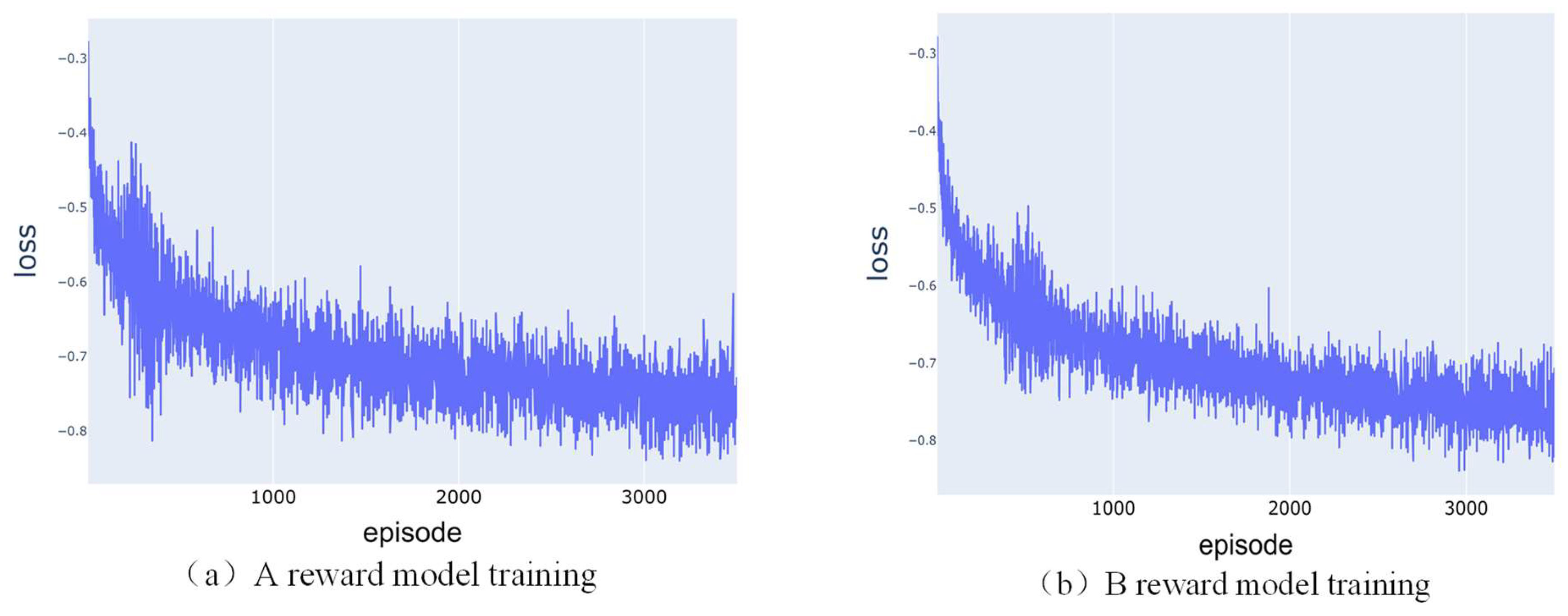
During the training process, the loss is calculated using the cross-entropy loss function, where a smaller the loss value indicates that the model output results are closer to the evaluation results of human feedback. During the training process, the Adam optimizer is used to update the parameters of the reward model, which minimizes the loss. Through iterative updates, an excellent reward model can be trained and used to guide the agent to obtain better performance in reinforcement learning tasks. Figure 7 shows the loss curves of the reward model training process for agents A and B. It can be seen that the loss values at the end of training are both much smaller relative to the beginning.

Figure 7. Reward model loss curve.

After the reward model is trained with enough data, it is used instead of the reinforcement learning reward function to continue to fine tune the policy model. Then, the reward models corresponding to A and B are plugged into the original training process to obtain two agents with different policies.

4.4. Assessment of Strategy Style Changes

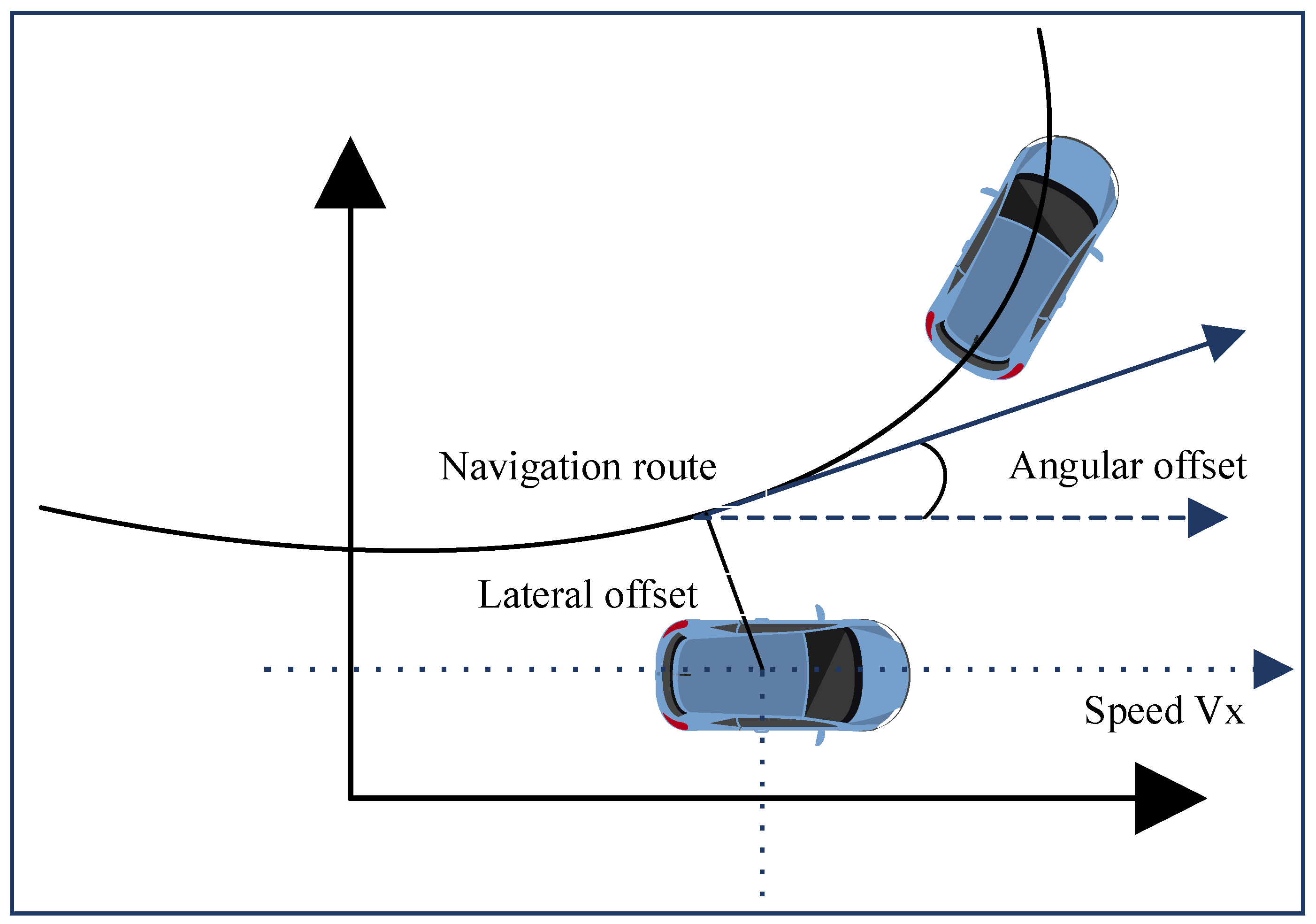
In order to measure the magnitude of the change in the strategy style of the two agents A and B after iteration and to ensure that the agents have learned the human style, the three features of average speed, average lateral offset, and average angular offset during the training iterations are used to construct vectors. The difference between different agents are measured by the Euclidean distance between the vectors, and the Euclidean distance is calculated as follows:

$$d\left(A,B\right)=\sqrt{{\sum }_{i=1}^n{\left(a_i-b_i\right)}^2}$$

(16)

where both A and B are n-dimensional vectors and $d\left(A,B\right)$ denotes the Euclidean distance between vectors A and B. It can be seen that the larger the similarity value, the smaller the difference between the two vectors and the higher the similarity.

During the fine-tuning process, every 1000 episodes, the average speed, average lateral offset, and average angular offset are calculated by testing with agents A and B and constructing the feature vectors. The following plots show the correlation coefficients of each agent style at the 1000th episode, the 2000th episode, the 3000th episode, and the 4000th episode. Both the horizontal and vertical coordinates are divided into four categories, and each cell indicates the similarity between the corresponding styles, the larger the value and the darker the color, the higher the similarity.

From Figure 8, it can be found that there are four different styles, namely, A_human, B_human, A_agent, and B_agent. A_human and B_human are based on the feature styles corresponding to human data, while A_agent and B_agent are the feature styles corresponding to the data generated by the agent as the training time increases. At the beginning, the similarity between A_agent and B_agent in Figure 8a is 0.86, which means that the style gap between them is not big. However, with the increase in training time, the similarity between A_agent and B_agent in Figure 8d becomes 0.23, which indicates that the style gap between them becomes larger. Meanwhile, the style gap between A_agent and A_human increases from 0.3 to 0.76, and the style similarity between B_agent and B_human increases from 0.29 to 0.63, indicating that after fine-tuning, two different styles of agents are indeed produced and that these two agents are much closer to A_human and B_human humans, respectively.

Figure 8. Heat map of style changes.

5. Testing and Verification of Personalized Control Strategies for Autonomous Vehicles

In order to verify the effectiveness of the algorithm established in this paper, A_agent and B_agent with 4000 episodes of parameter fine-tuning in the previous section are used as agents A and B, respectively, to verify whether agent A is relatively aggressive and if agent B is relatively stable through the simulation of typical traffic scenarios.

5.1. Crossroad Test

A schematic diagram of the intersection scene is shown in Figure 9, where the red dot is the starting point, the black dot is the target point, and the blue color is the desired route. Among them, the traffic light triggering condition is set to change to red automatically for 5 s when the agent approaches the intersection crosswalk within 5 m. In addition, the experiment chooses to generate a pedestrian crossing 10 m in front of the vehicle in the straight lane 6 s after the vehicle starts.

Figure 9. Intersection scene.

Figure 10 shows the different performances of the vehicles controlled by the two agents when confronted with a pedestrian, with the performance of agent A shown in Figure 10, A1 to A4, and the performance of agent B shown in Figure 10, B1 to B4, A1–A4 and B1–B4 show the travelling modes of agent A and agent B, respectively, when a pedestrian crossing occurs. The black vehicle is the vehicle controlled by the agent, the white person is the pedestrian crossing the road, and the blue dotted line is the point given by the navigation, containing the coordinate information as well as the heading angle information.

Figure 10. Path diagram of driving on a straight road.

Figure 11 shows the speed diagrams of agents A and B during the driving period. At the beginning, both vehicles first accelerated to 5 m/s. At the seventh second, a pedestrian appeared in front of them to cross the road, and vehicle B chose to stop immediately and wait for the pedestrian to pass, while vehicle A chose to slow down and go around gently before returning to the right direction to continue driving. After that, they both stop when facing the red light until the light turns green, and then accelerate to turn and pass the intersection.

Figure 11. Speed of an intersection.

Figure 12 and Figure 13 show the lateral offset and the angular offset variation curves, respectively. It can be seen that when driving in a straight line, agent B hardly deviates from the straight line, and agent A is obviously more likely to deviate from the trajectory. When driving around corners, both have a larger offset, but agent A offsets more. The tracking error performance of the two agents is shown in Table 5. The comparison shows that the average speed of agent A is faster than B, and the average lateral offset error and average angular offset error are also larger than B, indicating that the driving style of agent A is more aggressive than B.

Figure 12. Crossroad lateral offset curve.

Figure 13. Crossroad angular offset curve.

Table 5. Crossroad tracking performance.

Agent	Average Lateral Offset Error (m)	Average Angular Offset Error (rad)	Lateral Offset Error Variance	Angular Offset Error Variance	Average Speed
A	1.03238	0.18579	0.76003	0.20348	3.956
B	0.78507	0.05178	0.75048	0.06930	3.505

5.2. Comprehensive Evaluation Test

In order to improve the comprehensiveness and accuracy of the test and to evaluate the driving efficiency and safety of the different styles of agents, this section conducts a comprehensive evaluation experiment with traffic flow as the variable. It selects the TOWN01 map, which is different from the training map used in the experiment, to confirm whether they also reflect the style differences on different maps. The test metrics include vehicle speed, number of collisions, and tracking error. The red light is turned off in the experiment in order to assess the vehicle speed accurately, and only the number of vehicle collisions is recorded, which does not cause experiment failure.

Figure 14 shows the comparison curves of the average speed and the number of collisions under the two styles. From Figure 14a, it can be seen that the average speed of agent A is always larger than that of B under different traffic flows, while the speed difference between the two driving styles increases first and then decreases with the increase in traffic flows. From Figure 14b, it can be seen that agent B always maintains a relatively low number of collisions, while agent A has a relatively high number of collisions. This indicates that the driving style of agent A is more aggressive, while the driving style of agent B is more stable.

Figure 14. Comparison of average speed and number of collisions on the TOWN0 map.

Figure 15 shows a comparison of the tracking errors of the two agents under different traffic flows. It can be seen that the offset of A is larger than that of B at any time, and the magnitude of change in A is also more drastic. Table 6 shows a comparison of the mean value of the offset as well as the standard deviation of A and B under different traffic flows. The standard deviation reflects the degree of dispersion of the data, and it can be seen that the standard deviation of A is much larger than that of B, which indicates that the data of A fluctuates more. These results may be caused by factors such as the frequent overtaking of A.

Figure 15. Comparison of lateral offset and angular offset on the TOWN01 map.

Table 6. TOWN01 track error indicators.

Agent	Average Lateral Offset (m)	Average Angular Offset (rad)	Standard Deviation of Lateral Offset	Standard Deviation of Angular Offset
A	0.31374	0.05841	0.02116	0.01349
B	0.23494	0.04039	0.01205	0.00815

Through the simulation of typical scenes, the choices made by an agent in different scenes are compared. The results show that the two agents can still maintain their respective driving styles in different scenes, and the radical A-style vehicle is better at overtaking vehicles and overtaking pedestrians. However, the stable B-style vehicle is more willing to stop to avoid pedestrians and follow cars, which proves that the DDPG algorithm based on human feedback established in this paper is effective.

6. Conclusions

Based on the deep reinforcement learning algorithm with human feedback, this paper proposes an efficient and personalized decision control algorithm for autonomous vehicles. The algorithm combines two reinforcement learning algorithms, DDPG and PPO, and divides the control scheme into three phases including the pre-training phase, the human evaluation phase, and the parameter optimization phase. In the pre-training phase, the algorithm uses the DDPG algorithm to train an agent. In the human evaluation phase, the agent uses different trajectories generated by the DDPG algorithm to allow for different styles of people to rate them and, in turn, train their respective reward models based on the trajectories. In the parameter optimization phase, the network parameters are updated using the PPO algorithm and the reward values given by the reward models. Ultimately, the algorithm can adapt to different styles of people and give personalized decision-control solutions while ensuring safety.

Different behaviors of autonomous vehicles in avoiding pedestrians and vehicles in the face of intersections and complex traffic flow are tested through typical scenario experiments. The experimental results show that the algorithm can provide personalized decision-control solutions for different styles of people and satisfy human needs to the maximum extent while ensuring safety.

Driving style can be very complex. At present, only three dimensions of feature vectors are used in this paper to judge user preference. In future research, a deeper network structure and a more complex reward model can be tested to obtain better performance. At the same time, more feature data can be considered to judge the user preference so as to satisfy the user’s needs better.

References

- Pan, H.; Sun, W.; Sun, Q.; Gao, H. Deep learning based data fusion for sensor fault diagnosis and tolerance in autonomous vehicles. Chin. J. Mech. Eng. 2021, 34, 72. [Google Scholar] [CrossRef]
- Suzdaleva, E.; Nagy, I. An online estimation of driving style using data-dependent pointer model. Transp. Res. Part C Emerg. Technol. 2018, 86, 23–36. [Google Scholar] [CrossRef]
- Sagberg, F.; Selpi; Bianchi, P.G.F.; Johan, E. A review of research on driving styles and road safety. Hum. Factors 2015, 57, 1248–1275. [Google Scholar] [CrossRef]
- Aljaafreh, A.; Alshabatat, N.; Al-Din, M.S.N. Driving style recognition using fuzzy logic. In Proceedings of the IEEE International Conference on Vehicular Electronics and Safety (ICVES), Istanbul, Turkey, 24–27 July 2012; pp. 460–463. [Google Scholar]
- Chu, H.; Zhuang, H.; Wang, W.; Na, X.; Guo, L.; Zhang, J.; Gao, B.; Chen, H. A Review of Driving Style Recognition Methods from Short-Term and Long-Term Perspectives. IEEE Trans. Intell. Veh. 2023, 8, 4599–4612. [Google Scholar] [CrossRef]
- Gindele, T.; Brechtel, S.; Dillmann, R. Learning Driver Behavior Models from Traffic Observations for Decision Making and Planning. Intell. Transp. Syst. Mag. IEEE 2015, 7, 69–79. [Google Scholar] [CrossRef]
- Chen, Z.J.; Wu, C.Z.; Zhang, Y.S.; Huang, Z.; Jiang, J.F.; Lyu, N.C.; Ran, B. Vehicle Behavior Learning via Sparse Reconstruction with l2-lp Minimization and Trajectory Similarity. IEEE Trans. Intell. Transp. Syst. 2017, 18, 236–247. [Google Scholar] [CrossRef]
- Yang, W.; Zheng, L.; Li, Y.L. Personalized Automated Driving Decision Based on the Gaussian Mixture Model. J. Mech. Eng. 2022, 58, 280–288. [Google Scholar]
- Abdul, W.; Wen, T.G.; Kamaruddin, N. Understanding driver behavior using multi-dimensional CMAC. In Proceedings of the 2007 6th International Conference on Information, Communications & Signal Processing, Singapore, 10–13 December 2007; pp. 1–5. [Google Scholar]
- Yan, W. Research on Adaptive Cruise Control Algorithm Mimicking Driver Speed Following Behavior. Ph.D. Thesis, Jilin University, Changchun, China, 2016. [Google Scholar]
- Wang, W.; Zhao, D.; Han, W.; Xi, J. A learning-based approach for lane departure warning systems with a personalized driver model. IEEE Trans. Veh. Technol. 2018, 67, 9145–9157. [Google Scholar] [CrossRef]
- Li, A.; Jiang, H.; Zhou, J.; Zhou, X. Learning Human-Like Trajectory Planning on Urban Two-Lane Curved Roads From Experienced Drivers. IEEE Access 2019, 7, 65828–65838. [Google Scholar] [CrossRef]
- Ramyar, S.; Homaifar, A.; Salaken, S.M.; Nahavandi, S.; Kurt, A. A personalized highway driving assistance system. In Proceedings of the 2017 IEEE Intelligent Vehicles Symposium (IV), Los Angeles, CA, USA, 11–14 June 2017. [Google Scholar]
- Zhu, B.; Yan, S.; Zhao, J.; Deng, W. Personalized lane-change assistance system with driver behavior identification. IEEE Trans. Veh. Technol. 2018, 67, 10293–10306. [Google Scholar] [CrossRef]
- Huang, C.; Lv, C.; Hang, P.; Xing, Y. Toward safe and personalized autonomous driving: Decision-making and motion control with DPF and CDT techniques. IEEE/ASME Trans. Mechatron. 2021, 26, 611–620. [Google Scholar] [CrossRef]
- Zhu, M.; Wang, X.; Wang, Y. Human-like autonomous car-following model with deep reinforcement learning. Transp. Res. Part C Emerg. Technol. 2018, 97, 348–368. [Google Scholar] [CrossRef]
- Wang, X.P.; Chen, Z.J.; Wu, C.Z.; Xiong, S.G. A Method of Automatic Driving Decision for Smart Car Considering Driving Style. J. Traffic Inf. Saf. 2020, 2, 37–46. [Google Scholar]
- Behnaz, H.; Alireza, K.; Pouria, S. Deep reinforcement learning for adaptive path planning and control of an autonomous underwater vehicle. Appl. Ocean Res. 2022, 129, 103326. [Google Scholar]
- David, S.; Guy, L.; Nicolas, H.; Thomas, D. Martin Riedmiller Deterministic policy gradient algorithms: International conference on machine learning. Int. Conf. Mach. Learn. 2014, 32, 387–395. [Google Scholar]
- Griffith, S.; Subramanian, K.; Scholz, J.; Charles, L.I.; Thomaz, A.; Amodei, D. Policy shaping: Integrating human feedback with reinforcement learning. Adv. Neural Inf. Process. Syst. 2013, 26, 1–9. [Google Scholar]
- Christiano, P.F.; Leike, J.; Brown, T.B.; Martic, M.; Legg, S. Deep reinforcement learning from human preferences. arXiv 2017, arXiv:1706.03741v3. [Google Scholar]
- Schulman, J.; Wolski, F.; Dhariwal, P.; Radford, A.; Klimov, O. Proximal policy optimization algorithms. arXiv 2017, arXiv:1707.06347. [Google Scholar]
- Lillicrap, T.P.; Hunt, J.J.; Pritzel, A.; Heess, N.; Erez, T.; Tassa, Y.; Silver, D.; Wierstra, D. Continuous control with deep reinforcement learning. arXiv 2015, arXiv:1509.02971. [Google Scholar]
- Chen, J.; Li, S.E.; Tomizuka, M. Interpretable end-to-end urban autonomous driving with latent deep reinforcement learning. IEEE Trans. Intell. Transp. Syst. 2021, 23, 5068–5078. [Google Scholar] [CrossRef]
- Brockman, G.; Cheung, V.; Pettersson, L. Openai gym. arXiv 2016, arXiv:1606.01540. [Google Scholar]
Disclaimer/Publisher’s Note: The statements, opinions and data contained in all publications are solely those of the individual author(s) and contributor(s) and not of MDPI and/or the editor(s). MDPI and/or the editor(s) disclaim responsibility for any injury to people or property resulting from any ideas, methods, instructions or products referred to in the content. |
© 2024 by the authors. Licensee MDPI, Basel, Switzerland. This article is an open access article distributed under the terms and conditions of the Creative Commons Attribution (CC BY) license (https://creativecommons.org/licenses/by/4.0/).