Article

Context Awareness Assisted Integration System for Land Vehicles

by
Xiaoyu Li
,
Xiye Guo
*,
Kai Liu
,
Zhijun Meng
,
Guokai Chen
,
Yuqiu Tang
and
Jun Yang
College of Intelligence Science and Technology, National University of Defense Technology, Changsha 410073, China
*
Author to whom correspondence should be addressed.
Electronics 2024, 13(11), 2038; https://doi.org/10.3390/electronics13112038
Submission received: 21 March 2024 / Revised: 14 May 2024 / Accepted: 22 May 2024 / Published: 23 May 2024

Abstract

:
Accurate context awareness of land vehicles can assist integrated navigation systems. Motion behavior recognition is one context awareness of vehicles, based on which constraint information helps reduce the impact of short-term blockage of navigation signals on radio-frequency-based positioning systems. To improve the reliability of behavior recognition, we proposed a machine learning-based vehicle motion behavior recognition and constraint method (MLMRC). The machine learning-based recognition process is directly driven by raw data from low-cost MEMS-IMU, while the traditional threshold-based method relies on previous experience. Four categories of constraint information—sensor error calibration, velocity constraint, angle constraint, and position constraint—were constructed from the recognition results. Both the simulated vehicle experiment and real vehicle experiment demonstrate the performance of the MLMRC method. When there is a short-term blockage, the MLMRC method can reduce the positioning error from 17.2% to 38.3% compared with the traditional method, which effectively improves positioning accuracy and provides support for autonomous vehicles in complex urban environments.

1. Introduction

Location-based services help vehicle users travel to a specific destination in unfamiliar environments, especially for autonomous vehicles with extra requirements of safety and positioning accuracy [1]. The global navigation satellite system (GNSS) has been widely used in fields such as the Internet of Vehicles and autonomous driving [2].
However, GNSS-based positioning services have many limitations regarding accuracy, reliability, and continuity [3]. Vehicles often shuttle through urban canyons composed of high-rise buildings or travel to underground parking lots and tunnels. In the above environment, GNSS signals are easily blocked. It may lead to decreased positioning accuracy and even an inability to provide positioning services. To improve positioning performance in complex urban environments, positioning systems are generally equipped with inertial navigation systems (INS) [4]. INS relies on an inertial measurement unit (IMU) to perceive the acceleration and angular velocity of the vehicle and calculate its position, velocity, and attitude. To reduce the cost and power consumption of INS, low-cost MEMS-IMUs based on micro electro mechanical systems are widely used in integration systems. However, due to the high noise of MEMS-IMU, when GNSS cannot work, the positioning error of INS increases sharply over time. Such a phenomenon will lead the navigation system not to be able to meet the long-term high-precision positioning requirements [5].
One solution to overcome the increasing positioning error problem of INS is to add additional navigation sensors, such as odometers and electronic compasses [6]. If the measurement error of the above sensors is lower than the cumulative error of INS during the GNSS failure period, these external sensors can be utilized to correct INS. Li et al. utilized the three-axis attitude information from the magnetic compass to form external observations, which improves the observability of state variables and suppresses the accumulation of INS errors [7].
In addition to installing auxiliary sensors, geographic information can also be utilized for assistance. For example, using known altitude information to control the error growth of INS is an effective method when the number of visible satellites is less than four [8]. Establishing constraint equations based on the motion behavior of the carrier can also assist in correcting errors of INS, such as zero correction and the non-holonomic constraint method [9,10]. Sukkarieh proposed the non-holonomic constraint method to address the issue of correcting INS when GPS signals fail. When the carrier is a ground vehicle, under ideal conditions, its lateral and vertical velocities should be equal to zero. Based on that, a vehicle constraint equation can be established [5]. When the vehicle turns at a medium or high speed, due to the effect of lateral forces, there will be a lateral deviation between the wheels and the ground. At this time, the lateral velocity of the vehicle also needs to be considered. The constraint model needs to be improved by combining the front wheel deviation angle and wheel speed information output by the onboard sensors [8]. The combination of IMU measurements of different axes and wheel speed information can provide vehicle attitude constraints. The pitch angle can be calculated using gravity and vehicle acceleration, while the pitch angle can be jointly calculated using gravity, longitudinal velocity, lateral acceleration, pitch angle, and vertical angular velocity [11]. In addition to the angle, the velocity and position constraint equations were also extended by a new INS solution equation based on planar vehicle motion [12].
In recent years, with the development of intelligent control theory and artificial neural networks, some nonlinear data processing methods based on artificial intelligence (AI) have gradually been applied to integration systems [13]. In general, the commonality of the above methods is the modeling of the relationship between the output of INS and the error of INS based on AI models when GNSS is working. When GNSS fails, the INS error is predicted based on the established model and the INS output. Then the model is used to correct the output of INS which improves the positioning accuracy when GNSS is blocked. Such a method did not consider the historical development trend of INS error. So, when the GNSS blockage time is long, there will be significant prediction errors [14]. In addition, when the amount of data is insufficient, neural network methods cannot complete effective training [15].
Based on the comprehensive analysis of the three sorts of methods mentioned above, constructing constraint equations based on motion behaviors is easier to deploy. It does not require additional sensors in the positioning system. However, the method needs to detect the motion characteristics of the carrier in advance. The multi-sensor positioning system detects the status of the carrier and configures its positioning mode accordingly. This process is called context awareness. Context refers to various types of information closely related to the user terminal, such as time, geographical location, environment, behavior, etc., [16]. Among them, behavior refers to the movement behavior of the carrier. The flexible switching of positioning modes depends on changes in behavior. Through context awareness, user behavior can be judged. Then the corresponding positioning algorithm can be instructed to switch resiliently, which improves positioning accuracy and reliability [17,18]. For example, stationary vehicles have a fixed position and do not need to update their velocity and position. For GNSS receivers, behavior recognition can be used to adjust the bandwidth and coherence integration time of the tracking loop, as well as to predict the time characteristics of the multipath [19].
Based on the descriptions so far about reducing the impact of short-term blockage of navigation signals on radio-frequency-based positioning systems, the contributions of this article are summarized as follows:
(i) We propose a machine learning-based vehicle motion behavior recognition and constraint method (MLMRC). In the method, positioning constraint equations can be added to the navigation systems based on the motion behavior of the vehicles. It could suppress resiliently the accumulation of positioning errors caused by insufficient observation information.
(ii) Machine learning models are utilized to improve the reliability of motion behavior recognition and reduce the reliance on prior experience.
(iii) We aggregate available positioning constraint information for vehicles. Then, we divide the constraint information into four categories: sensor error calibration, velocity constraint, angle constraint, and position constraint. As for angle constraint, the theoretical relationship between predicted angle error and misalignment angle error predicted by INS is deduced.
(iv) As one of the enhancement and assistance methods when there are insufficient input signals, the MLMRC method modifies the proposed resilient PNT (Positioning, Navigation, and Timing) architecture of the Ground-based High-precision Local Positioning System (GH-LPS).
The remaining part of this paper is organized as follows. We introduce the related work in Section 2. In Section 3, the modified resilient PNT architecture and the modified integration model based on the proposed MLMRC method are constructed. Then the classification and recognition of vehicle motion behavior and the positioning constraint equations for tightly coupled integration are derived. Section 4 and Section 5 evaluate the performance of the MLMRC method using a moving platform traveling along a fixed track indoors and a testing vehicle driving in a long tunnel, respectively.

2. Related Work

2.1. Existing Methods

Constraint equations can be constructed by the recognition results of motion behaviors. Qin proposes a fuzzy interactive multiple model algorithm based on fuzzy rules. The method introduces feature variables directly related to the system model. Then, it formulates fuzzy rules to determine the selection probability of kinematic and dynamic vehicle models to improve the estimation accuracy of model probability [8]. Liu et al. divide motion behavior into three states based on motion speed: stationary (<0.1 m/s), low-speed (≥0.1 m/s, <10 m/s), and fast-speed motion (≥10 m/s), and design fuzzy logic rules to adjust adaptive Kalman filtering parameters [20]. Gao et al. utilize MEMS-IMU data to recognize vehicle motion behavior (stationary, straight, turning) for the motion constraint-aided method [15]. They achieve context awareness based on the angular velocity in the vertical direction (z-axis) and three-axis acceleration information. Vehicle experiments show that the recognition of vehicle context is beneficial for improving positioning accuracy. On this basis, they also verified the auxiliary effect of motion state recognition on PPP/INS tightly coupled integration [21]. Although the detection threshold can be adjusted online, it still requires manual setting of the initial values. As for vehicle constraint models, Wang pointed out that the measurement error of MEMS-IMU is relatively large. As a result, AI algorithms were introduced to identify the motion behavior of vehicles accurately [12]. Fuzzy logic is adopted to determine stationary, straight, and turn based on the values of acceleration and z-axis angular velocity. At the same time, external observation values are also combined to constrain the INS solution. Although an AI algorithm is used, fixed parameters that are artificially set are still used as feature judgment criteria.

2.2. Innovative Elements of the New Method

To reduce the reliance on prior information and improve the reliability of behavior recognition, we proposed the MLMRC method. The comparison of the MLMRC method and existing methods for constructing constraint equations based on the motion behaviors is given in Table 1. The MLMRC method proposed in this paper utilizes machine learning methods to recognize motion behaviors in any manual setting based on previous experience. Additionally, the proposed method only requires basic IMU sensors which are common in vehicle navigation systems.

3. Methodology

The proposed MLMRC method is a motion behavior recognition-based method. In addition, the MLMRC method aims to reduce the impact of short-term blockage of navigation signals on radio-frequency-based positioning systems. For the above reasons, the method should be deployed on a radio-frequency-based positioning system/INS integration. GH-LPS is a radio-frequency-based positioning and navigation system that operates similarly to GNSS and was proposed in our early research [22]. A tightly coupled integration model of GH-LPS/INS was constructed in the preliminary research [23]. A two-layer resilient PNT architecture of GH-LPS was created based on the GH-LPS/INS integration by our previous research, enabling GH-LPS to be highly resilient to untrusted input [24]. However, the created resilient PNT architecture only focuses on the untrusted input. It does not consider insufficient input situations such as signal blockage, which is also a commonly adverse factor influencing the positioning results of radio frequency-based positioning systems. To address this problem, a modified resilient PNT architecture of GH-LPS is proposed where the context awareness-assisted positioning method proposed in this paper serves as one layer in the architecture, as shown in Figure 1.
The outermost layer (yellow) assumes that any external input is untrusted. Aided by the IMU in the innermost layer (green), the outermost layer applies broadly applicable methods to detect anomalies, such as carrier phase measurement cycle slips. The modified resilient PNT architecture of GH-LPS adds a middle layer (blue) to assist and enhance PNT results when the input signals are not sufficient. When there is insufficient available information caused by the signal blockage or non-line-of-sight signal, optimization methods such as adding constraint equations can be selected based on the surrounding context to avoid the deterioration of positioning performance.
As an example of the middle layer of resilient PNT architecture, the MLMRC is added to the integration model, and the architecture of the integration system is shown in Figure 2. The module consists of two parts—context awareness and motion constraints—which are introduced in detail in Section 3.2 and Section 3.3, respectively. First, raw data from the accelerometer (ACC) and the gyroscope (GYO) are input into the context awareness module to form features. Subsequently, the context awareness module infers the vehicle’s motion behavior based on the established model constructed by the machine learning method, including the stationary, straight, and turning three motions. Finally, the motion constraint module forms corresponding constraint equations based on the vehicle’s motion behavior and adds them to the extended Kalman filter. This enriches the basic integration model and achieves resilient positioning in complex situations. Because the MLMRC module directly uses raw data from sensors and does not rely on any prior experience or manual settings, it can be added to any integration system containing IMU sensors to provide real-time context assistance information.

3.1. Basic Integration Model

The proposed MLMRC method forms the corresponding constraint equations to construct observation equations in the tightly coupled integration model according to the recognition results of motion behaviors. Therefore, it is necessary to introduce the basic integration model in advance.
The 17-state vector used includes navigation parameter errors (attitude error ε , velocity error δ v , position error δ r e ), the bias of the gyroscope δ b g and the accelerometer δ b a , estimation error of the receiver’s clock bias δ d t , and clock drift δ d f :
x n = [ ε δ v δ r e δ b g δ b a δ d t δ d f ] T .
The observation vector of Kalman filtering is composed of the residuals between the measurements and predictions of carrier phase and Doppler:
z 1 = [ ϕ I N S 1 ϕ Re c e i v e r 1 ϕ I N S M ϕ Re ceiver M D I N S 1 D Re ceiver 1 D I N S M D Re ceiver M ] ,
where, ϕ i is the carrier phase measurement in cycles and D i is the Doppler measurement whose superscript i refers to the corresponding positioning base stations ( M in total), and the subscript represents the INS prediction and receiver measurement, respectively.
Taking the derivative of the carrier phase observation equation and Doppler observation equation, the unknown variables to be solved are the receiver’s position coordinates ( x , y , z ) , clock bias d t , velocity v , and clock drift d f of the receiver. By linearizing the equations, the observation equation can be obtained [22,25]. Therefore, the observation matrix is the following:
C 1 = [ 0 M × 6 G T l n 0 M × 6 1 M × 1 0 M × 1 0 M × 3 G 0 M × 9 0 M × 1 1 M × 1 ] .
Because the receiver resolves the positioning solution in the local coordinate system ( l frame) while the Kalman filter state vectors are in n frame, a coordinate system conversion is also required:
T l n = [ 0 a cos λ 0 a 0 0 0 0 1 ] .

3.2. Behavior Recognition

The context awareness module recognizes the motion behavior in real time based on the raw data collected from the IMU. It helps to construct the corresponding constraint equations to be added to the extended Kalman filter to improve positioning performance. In this section, the motion behaviors of vehicles are studied and classified into three sorts of behaviors: stationary, straight, and turning, based on the applicable conditions of vehicle constraint equations. To overcome the problem of manual threshold setting relying on previous experience, and improving recognition accuracy and reliability, machine learning methods are used in behavior recognition due to less parameter tuning [26]. The vehicle motion behavior recognition problem belongs to the classification problem in supervised learning [27,28]. To effectively utilize the original measurements, it is necessary first to preprocess the raw data of accelerometers and gyroscopes and then convert them into several features that can reflect different motion behavior characteristics.
When using the measurements of three-axis accelerometers as recognition features, the output of the sensors may not necessarily be the same under the same motion behavior due to the differences in sensor installation angles and unevenness of the ground. To overcome this problem, the scalar parameters of the accelerometer measurements can be used as recognition features, including the scalar value of the acceleration and the absolute value of its variation within a specific statistical window. However, the scalarization processing mentioned above will lose the axial information contained in the accelerometer.
When the vehicle is moving, the horizontal accelerometer measurements change most significantly. Therefore, the variation characteristics of the horizontal axes of the accelerometer (assumed to be the x-axis and y-axis in b frame) within the statistical window are added as statistical features, including the standard deviation, the difference between the maximum and minimum values, and the difference between the maximum and minimum values of the standard deviation of the x-axis and y-axis accelerations.
In addition to accelerometers, the output of gyroscopes can also be used to recognize vehicle motion, where the vertical angular velocity can reflect the vehicle’s motion behavior. However, due to the presence of outliers caused by human factors, such as slight movement of the steering wheel, or non-human factors, such as getting on and off, it is necessary to filter the original gyroscope data. Therefore, the average z-axis angular velocity and the filtered z-axis angular velocity within the statistical window are used as classification features.
After analyzing the physical characteristics related to vehicle motion behavior, as shown in Table 2, a total of eleven features for motion behavior recognition are defined, of which eight features are from accelerometer measurements and three features are from gyroscope measurements.
Due to the limited sorts of motion behaviors and the small amount of data, machine learning algorithms are mainly considered. Typical machine learning classification algorithms include Discriminant Analysis (DA), Naïve Bayesian (NB), k-Nearest Neighbor (kNN), Decision Tree (DT), Random Forest (RF), and Support Vector Machine (SVM). The performance of different algorithms are analyzed and compared in the experiment.

3.3. Constraint Equations

The motion constraint module could utilize the measurements of sensors and state parameters of the integration system to further construct motion constraint equations, given the vehicle motion behaviors [8,12,21]. Available vehicle positioning constraint information is aggregated in this section and the constraint conditions are divided into four categories: sensor error calibration, velocity constraint, angle constraint, and position constraint. The usage conditions of the constraints are analyzed, and the corresponding equations are derived.

3.3.1. Sensor Error Calibration

Low-cost MEMS-IMU cannot maintain long-term high-precision measurement, so it is necessary to detect the outputs of the sensors and calculate the compensation parameters for sensor errors during positioning [29]. When the vehicle is stationary, regardless of whether the engine is turned on or not, since its position, velocity, and attitude remain unchanged, the outputs of the accelerometer and gyroscope can be considered as the sum of bias and noise:
f i b b = δ f b + C n b g n + η a w i b b = δ w b + η g ,
where, f i b b is the specific force vector measured by the accelerometer, w i b b is the angular velocity vector measured by the gyroscope, and g n is the local gravitational acceleration vector [15]. When the vehicle is moving in a straight line, the vertical angular velocity of the gyroscope can also be regarded as the sum of bias and noise. Based on sensor error calibration, the following measurement equation can be established:
z 2 = [ f i b b - C n b × g n w i b b ] ,
C 2 = [ 0 3 × 9 0 3 × 3 I 3 × 5 0 3 × 9 I 3 × 3 0 3 × 5 ] .

3.3.2. Velocity Constraint

The non-holonomic constraint method suggests that under ideal conditions, the lateral and vertical velocities of ground vehicles should be zero [5]. This condition applies to stationary, straight, and low-speed turns (there may be a sideslip during high-speed turns), meaning that the velocity of the x axis and z axis in b frame should be equal to zero. However, due to factors such as sensor errors, the actual speed will exhibit a certain degree of random deviation:
v x , I N S b = 0 + σ v x v z , I N S b = 0 + σ v z .
When the vehicle is stationary, the velocity is zero. Therefore, the velocities of each axis in b frame are all zero; that is, the y axis velocity is zero:
v y , I N S b = 0 + σ v z .
When the vehicle turns, there is a centripetal force so that the forward velocity can be calculated based on Newton’s equation:
v y b = f i b x b g cos θ sin ϕ w i b z b ,
where, θ and ϕ are pitch angle and roll angle, respectively. This constraint is only applicable when the turning speed is high and w i b z b is much greater than its noise. The following equation can be obtained by taking the derivative of the predicted velocity of INS and the calculated forward velocity separately:
δ v I N S b = C n b [ δ ε × ] v + C n b δ v = C n b [ v × ] δ ε + C n b δ v ,
δ v y b = 1 w i b z b ( 1 cos θ ) δ f i b x b 1 ( w i b z b ) 2 ( f i b x b + g cos θ sin ϕ ) δ w i b z b ,
where [ × ] represents the antisymmetric matrix.
Based on velocity constraints, the following measurement equation can be established:
z 3 = [ v x , I N S b v y , I N S b v y b v z , I N S b ] ,
C 3 = [ C n b [ v × ] C n b 0 3 × 11 ] .

3.3.3. Angle Constraint

Based on the measurements of the accelerometer and gravity projection, the roll angle can be calculated when the vehicle is stationary or in straight motion [12]:
ϕ = sin 1 ( f i b x b g ) .
The roll angle constraint error is as follows:
δ ϕ = 1 1 ( f i b x b / g ) 2 δ f i b x b .
When the vehicle is stationary, the heading angle remains unchanged:
γ I N S , t = γ I N S , t 1 + σ γ .
To construct the angle constraint equation, the theoretical relationship between predicted angle error and misalignment angle error ε = [ ε e ε n ε u ] predicted by INS is derived. The specific derivation process is shown in Appendix A:
𝜕 ϕ I N S 𝜕 ε e C ^ b n ( 3 , 3 ) C ^ b n ( 2 , 2 ) C ^ b n ( 3 , 1 ) C ^ b n ( 2 , 3 ) C ^ b n ( 3 , 1 ) 2 + C ^ b n ( 3 , 3 ) 2 ,
𝜕 ϕ I N S 𝜕 ε u = 0 ,
𝜕 γ I N S 𝜕 ε e C ^ b n ( 1 , 2 ) C ^ b n ( 3 , 2 ) C ^ b n ( 1 , 2 ) 2 + C ^ b n ( 2 , 2 ) 2 ,
𝜕 γ I N S 𝜕 ε n C ^ b n ( 2 , 2 ) C ^ b n ( 3 , 2 ) C ^ b n ( 1 , 2 ) 2 + C ^ b n ( 2 , 2 ) 2 ,
𝜕 γ I N S 𝜕 ε u 1 ,
where, γ is the heading angle, and C ^ b n , is the directional cosine matrix predicted by INS:
C ^ b n = [ I ( ε × ) ] C b n .
Based on angle constraints, the following measurement equation can be established:
z 4 = [ ϕ I N S asin ( f i b x b / g ) γ I N S , t γ I N S , t 1 ] ,
C 4 = [ 𝜕 ϕ I N S 𝜕 ε e 𝜕 ϕ I N S 𝜕 ε n 𝜕 ϕ I N S 𝜕 ε u 0 1 × 14 𝜕 γ I N S 𝜕 ε e 𝜕 γ I N S 𝜕 ε n 𝜕 γ I N S 𝜕 ε u 0 1 × 14 ] .

3.3.4. Position Constraint

When the vehicle is moving on a horizontal plane or with the assistance of an elevation map, unknown parameters can be reduced just by adding constraints in the height direction [30]. Tide gauges can be used at sea, barometers can be used in the air, and prior elevation coordinates can be used on horizontal ground.
Based on positional constraints, the following measurement equations can be established:
z 5 = [ H I N S H cos traint ] ,
C 5 = [ 0 2 × 8 1 0 2 × 8 ] ,
where H cos traint is the height constraint in n frame.
According to the four categories of constraint types and their usage conditions, the relationship between different motion behaviors and applicable vehicle constraint equations is shown in Table 3:

4. Simulated Vehicle Experiment

4.1. Experiment Setup

To verify the effectiveness of the MLMRC method, a set of GH-LPS was installed on a semi-enclosed basketball court. As shown in Figure 3, a total of four base stations (BS 1–BS 4) were used in the experiment, fixed on the support of the basketball court ceiling. The user receiver was mounted on a moving platform traveling in circles along the fixed track, which consisted of two straight segments and two curved segments, simulating a vehicle, as shown in Figure 4. Its maximum speed was maintained at around 1 m/s. The coordinates of the transmitting antennas of each base station are listed in Table 4, measured by a total station set next to the court. The coordinates are in the East-North-Up (ENU) frame which is a local frame centered in the total station [31]. The average horizontal dilution of precision value throughout the environment is approximately 1.16. It is worth noting that the carrier phase measurements, Doppler measurements, and IMU measurements used in this experiment were all from the raw data output by the user receiver. The MEMS-IMU LINS16460 was installed inside the receiver, with built-in accelerometers and gyroscopes of bias stability 10 μ g and 4°/h, respectively, and the velocity random walk and angle random walk are 0.05 m/s/√h and 0.3 °/√h, respectively.

4.2. Data Collection

Two separate sets of experimental data are selected for training and testing, respectively. Each data set contains three sorts of motion: stationary, straight, and turning. The raw data from the accelerometer and gyroscope are shown in Figure 5 and Figure 6, respectively. It can be seen that there are differences in amplitude between the training and testing data under the same behavior, and even differences exist between the data under the same behavior in the training set. On the one hand, the tilt angle is different because the platform is in various positions, which causes changes in the projection components of gravity on each axis when the platform is stationary. On the other hand, factors such as vibration during the experiment may generate certain outliers, which may affect the purity of the data.

4.3. Recognition Results

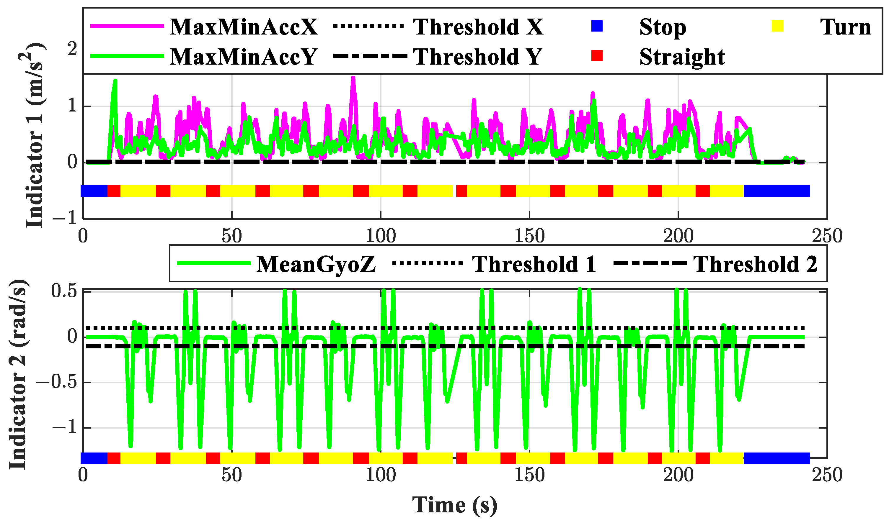
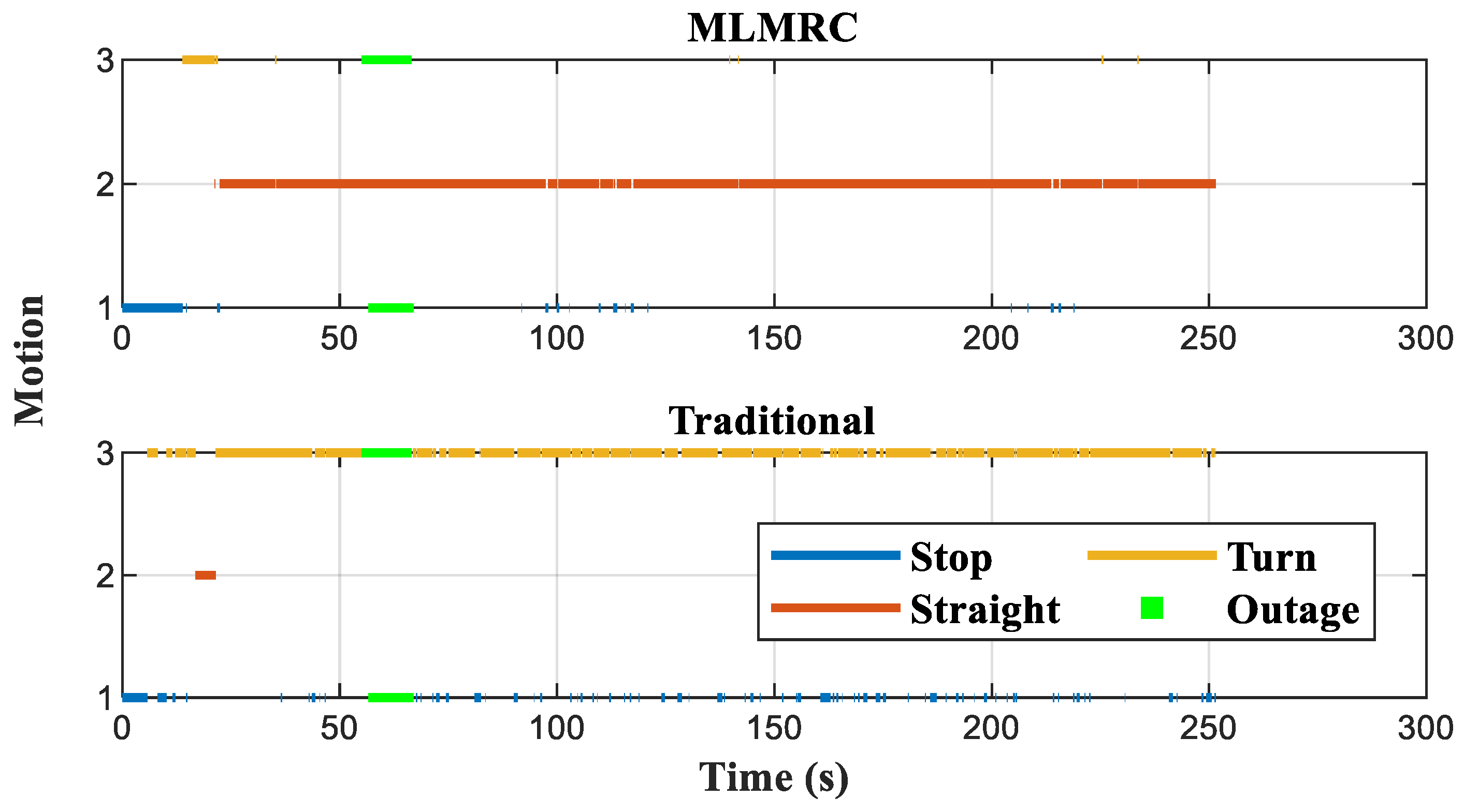
4.3.1. Traditional Threshold-Based Method

The traditional method refers to the following threshold-based method. Gao et al. use the standard deviation of accelerometer measurements within a fixed time window to determine whether the vehicle is stationary or not and use vertical axis gyroscope measurements to determine two types of vehicle movements: turning and straight [15]. Thus, criterion 1 and criterion 2 correspond to Formulas (7) and (9) in reference [15], respectively. The window length is set to 1.5 s according to the literature, and the recognition results are shown in Figure 7. When the platform is stationary, the statistics constructed by criterion 1 (MaxMinAccX and MaxMinAccY) are significantly smaller than those in the dynamic motion, which can effectively determine whether the platform is stationary or not. For criterion 2, when the platform moves in a straight line, the statistics (MeanGyoZ) are relatively flat and different from that in the turning motion. However, it is worth noting that the movement of the platform is continuous, as shown in criterion 2. Although it is possible to ensure that there are no omissions in recognition of straight motion by setting two thresholds, there will always be some non-straight motions that are misclassified as straight motions, which can lead to incorrect positioning constraints and pose risks. In addition, there are also certain times when the statistics are false due to outliers, vibrations, etc. Therefore, although different motion behaviors can be distinguished by constructing thresholds, it is not easy to set appropriate recognition thresholds in the face of actual data to ensure that all motion behaviors can be accurately classified.

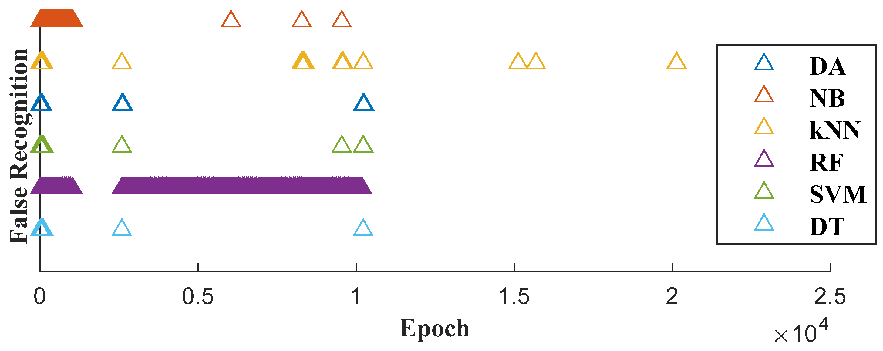
4.3.2. Machine Learning-Based Method

In response to the above issues, the machine learning-based motion behavior recognition method proposed in this paper is validated using the same dataset. The input features of the classifier are the eleven features in Table 4 (with a window time of one second and filter weights of 100). A LEGION R9000X laptop made by Lenovo Group in Beijing, China (AMD Ryzen 7 4800H, Radeon Graphics 2.90 GHz, RAM 23.4 GB) was used. First, the performance of different machine learning algorithms is compared. The six typical machine learning classifiers, DT, DA, NB, kNN, RF, and SVM, are constructed in MATLAB (R2020a). The performance of the six classifiers is compared based on three parameters: training time, training accuracy, and test accuracy, which are shown in Table 5. From the perspective of application, it is necessary to ensure high data rates and high test accuracy. From the perspective of training time, there is a significant difference of one order of magnitude between RF and SVM two classifiers and other classifiers. From the perspective of accuracy indicators, except for the low training accuracy of RF (about 90%), the performance of other algorithms is excellent (about 99%). However, high training accuracy does not necessarily mean better performance. If overfitting is caused, it is not conducive to improving test accuracy, such as the test accuracy of NB reduces by about 30% compared to training accuracy. Figure 8 illustrates the false point in recognition of different machine learning methods, it can be seen that except for various false points of NB and RF, most of the other false points of different methods show a similar pattern around certain epochs.
The recognition results of machine-learning methods demonstrate that, except for specific indicators of individual methods, the overall performance of each machine-learning algorithm is on the same level, showing good applicability. Introducing deep learning methods will increase computational time, and it is not easy to achieve higher recognition accuracy. Among the above machine algorithms, the main advantages of DT are that the model is readable and has a fast classification speed [32]. Gao et al. applied the DT algorithm in smartphone sensors such as accelerometers, gyroscopes, magnetometers, and barometers to distinguish human activities from vehicle movements [28]. Therefore, the DT algorithm was selected as a typical representative for the classification algorithm used for vehicle motion behavior recognition in the following analysis.

4.3.3. Summary of Recognition Results

The results of the traditional method and behavior recognition based on DT are shown in Figure 9. The recognition results indicate that the moving platform is first in stationary motion and then repeatedly moved in a “straight-turning” pattern until it stops, which is consistent with the actual trajectory. Except for misjudgment occurring around 100 s and wrongly classifying straight motion as stationary motion, all other results are consistent with actual motion behaviors. However, the traditional threshold-based method often fails to recognize motions, leading to frequent switching between straight and turning motions.
The confusion matrix for motion behavior recognition results based on the DT algorithm is acquired by MATLAB. The comparison of the recognized results and labeled ones is shown in Table 6, with an accuracy of 99.0%, an improvement of about 6% compared to the traditional method’s 93.6% result. Additionally, the recognition results of the two methods in previous sections demonstrate that the results of the DT algorithm are more continuous and reliable. The subsequent positioning performance analysis further demonstrates its improvement effect.

4.4. Positioning Results

As for the radio frequency-based positioning system, when the number of available signals drops below the minimum requirement, there is insufficient available information to correct the error of the INS, and there will be error accumulation. The variation in the dilution of precision caused by different remaining available signals affects the accumulation speed of errors. At the same time, a virtual constraint equation can be constructed based on the real-time motion recognition results to provide additional auxiliary positioning information and decrease the accumulation. Based on the previous section on motion behavior recognition, the suppression effect of the MLMRC method on error accumulation under different conditions when the available signal is insufficient is explored. During the experiment, the moving platform ran around a fixed track containing both straight and curved segments. To avoid randomness, five different positions in the trajectory are selected as the start points for signal blockage with a manual 10-s signal blockage simulation. The receiver positions at the start time of each blockage and the motion behavior within each blockage interval are shown in Figure 10 and Figure 11, respectively. It can be seen that, in the selected five blockage intervals, there are two types of segments—straight segment and curved segment—and three sorts of motion behaviors—stationary, straight, and turning—are all included.
To explore the performance of the MLMRC method, the traditional threshold-based method under different available signal conditions, four typical cases are selected for analysis: single base station (BS 1), dual base stations (BS 1 and BS 2), three base stations (BS 1–3), and all four base stations blockage.

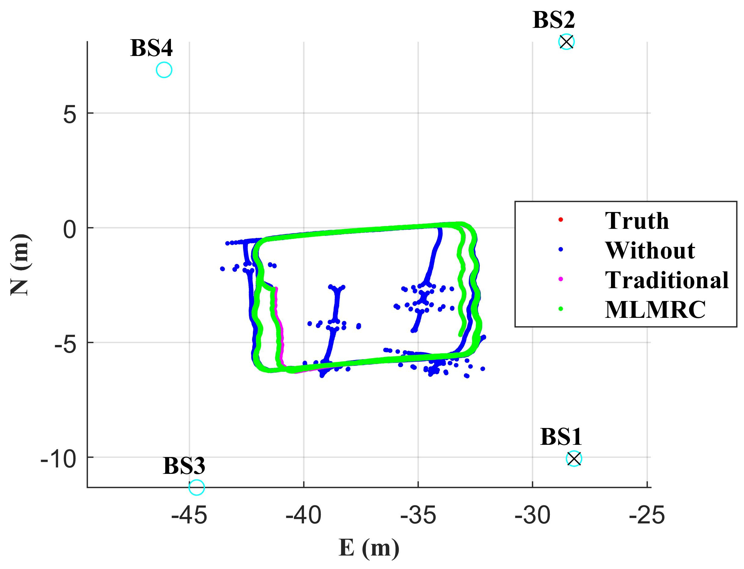
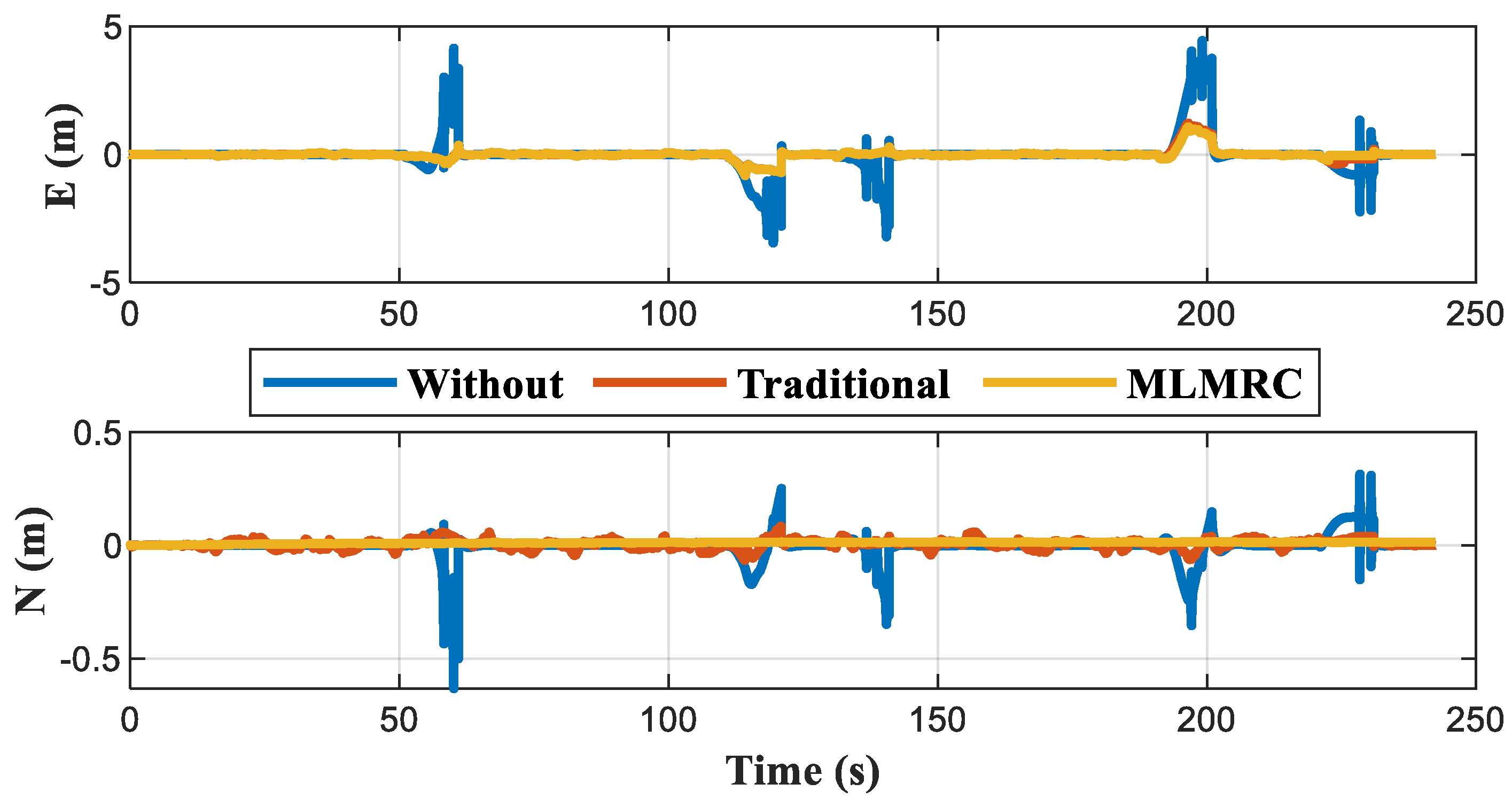
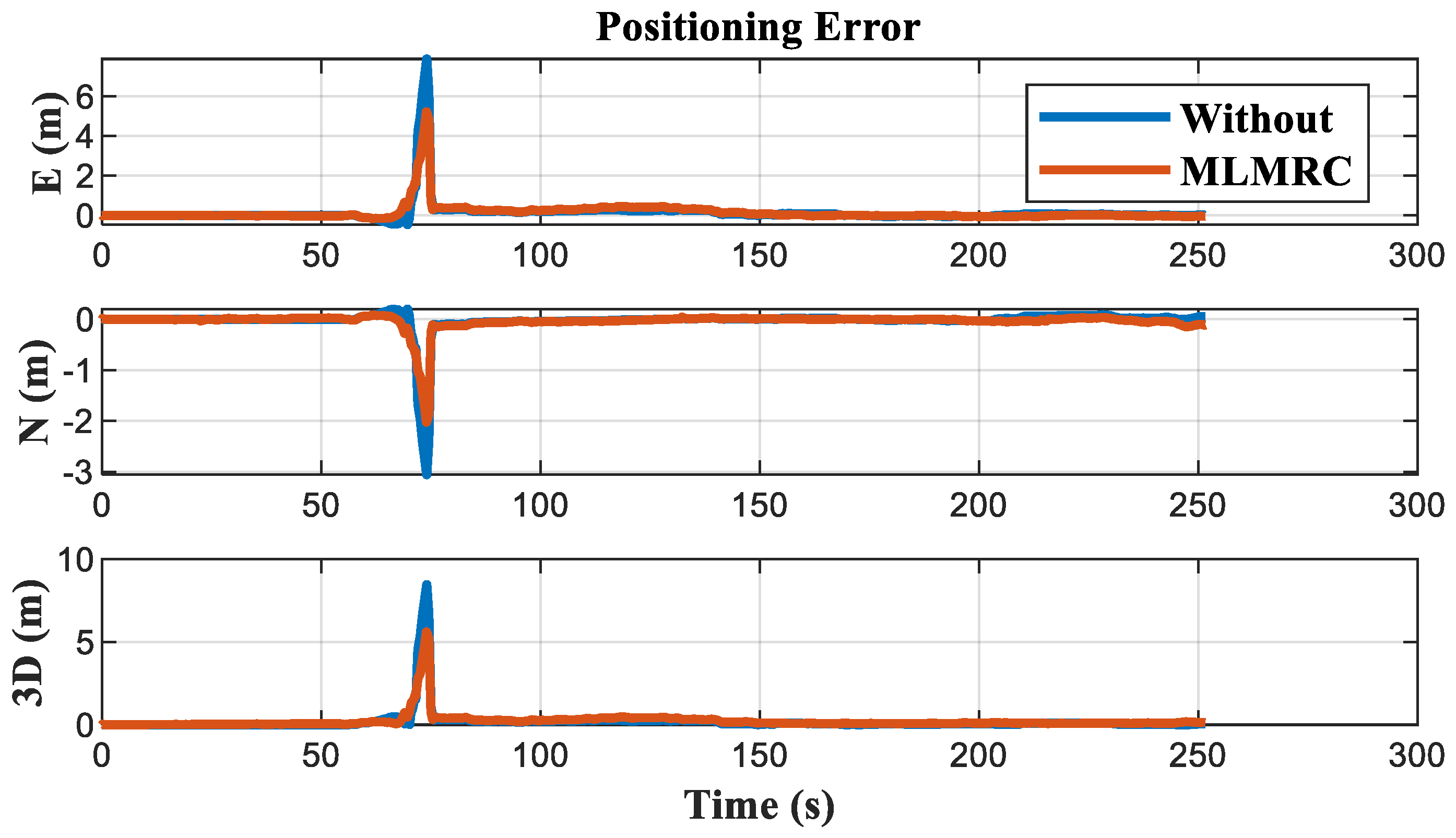
4.4.1. Single Base Station Blockage Condition

For horizontal positioning using height constraints, a minimum of three available base station signals needs to be ensured to meet the positioning requirements. Therefore, in the case of a single base station blockage, adding the constraint equations does not improve the performance. As shown in Figure 12, there is no significant difference between the positioning trajectories of each method, which coincides with the truth. However, the N-direction positioning error in Figure 13 indicates that the positioning error of MLMRC is more continuous and smoother compared to the traditional method due to its reliable motion recognition results. The max, min, and root mean square (RMS) values of the positioning errors within five blockage intervals are presented in Table 7. These results in E, N, and horizontal (2D) demonstrate that the performance of different methods is similar and remains at the centimeter level.

4.4.2. Dual Base Stations Blockage Condition

The positioning results where dual base stations are blocked simultaneously are shown in Figure 14. When the signal is blocked, the positioning error begins to accumulate until the blockage end time, where the positioning error quickly decreases and returns to the centimeter level. Although the cumulative rate of positioning error varies at different start positions, as shown in Figure 15, when there is a signal blockage, the positioning results of MLMRC methods are more accurate due to the correct usage of positioning constraint equations. The statistical results in Table 8 indicate that the root mean square (RMS) error of the MLMRC method decreased from 151.0 cm in the E direction without any constraints to 39.5 cm and from 12.9 cm to 2.9 cm in the N direction. Compared to the traditional threshold-based method, the horizontal RMS and maximum positioning error of the MLMRC method have been increased to 39.6 cm and 107.0 cm, respectively.

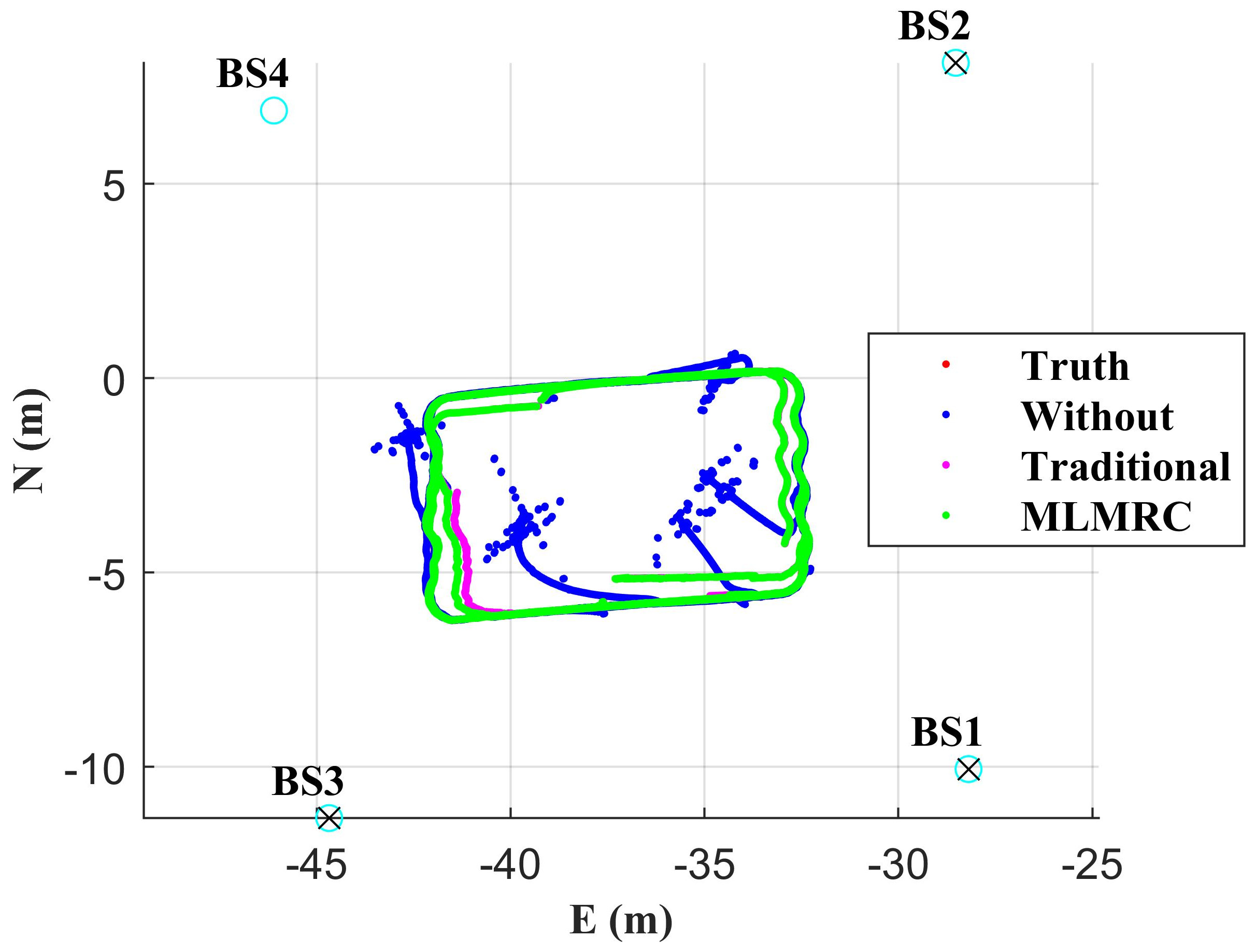
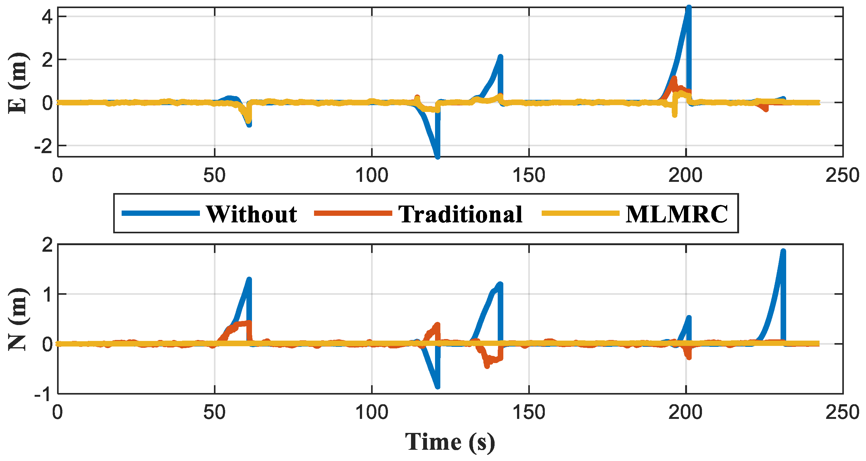
4.4.3. Three Base Stations Blockage Condition

For the case where three base stations are blocked simultaneously as shown in Figure 16, compared to the dual base station blockage condition, there is only one available base station left, and the available information is further reduced. However, the positioning errors shown in Figure 17 and Table 9 indicate that the RMS error of the MLMRC method in the E direction, N direction, and horizontal direction has decreased to 24.3%, 17.2%, and 20.5% of the case without any constraints, respectively. Furthermore, compared to the traditional threshold-based method, the maximum and RMS horizontal error of the MLMRC method have been reduced by 38.3% and 20.0%, respectively.

4.4.4. All Four Base Stations Blockage Condition

When all four base stations are blocked, there is no available information to correct the cumulative error of INS, and the positioning results are shown in Figure 18. Figure 19 further indicates that the positioning error within each blockage interval continues to increase over time. After adding the positioning constraint equations, the horizontal positioning error of the MLMRC method is only 82.8% (maximum) and 78.5% (RMS) of the traditional method. The RMS of the error in E and N directions are reduced to 20.4 cm and 18.9 cm, respectively, as shown in Table 10, which is much smaller than the 116.2 cm and 58.8 cm before using constraints.

4.4.5. Summary of Positioning Results

The positioning results of the single base station blockage condition show that when the number of available signals meets the minimum positioning requirements, using a constraint equation based on motion behavior recognition results does not improve the positioning performance. The positioning results of other blockage conditions demonstrate that, when the number of available signals does not meet the minimum requirement, the MLMRC method significantly improves positioning accuracy. Although the cumulative error of the tight integration system varies at different positions under different combinations of base stations, the MLMRC method can reduce the positioning error (max error) from 17.2% to 38.3% compared with the traditional method.

5. Real Vehicle Experiment

5.1. Test Area

A vehicle experiment was conducted in a highway tunnel in Beijing, China. The testbed consists of a total of 34 GH-LPS base stations installed at the top of the tunnel, as shown in Figure 20, and the layout is shown in Figure 21. The coordinates of the base stations’ transmitting antennas were calibrated by a total station, and the lane-level positioning results without any simulated signal blockage were used as the reference [33].
The user terminal was mounted on the top of the testing vehicle (an average speed of 74.48 km/h moving in the tunnel) and consisted of two receivers with a separate receiving antenna, as shown in Figure 20. The fixed baseline between the two receivers is used to evaluate positioning accuracy. The MEMS-IMU LINS16460 is integrated inside the receiver.

5.2. Simulated Signal Blockage

Due to the limitation of the physical visibility of line-of-sight signals by the curved tunnel, the receiver may receive non-line-of-sight signals, resulting in positioning errors. However, if the number of base stations used in the positioning is directly limited based on the distance between the base station and the user terminal, it may result in the number of available signals being lower than the minimum requirements for positioning, leading to an increase in positioning error. In addition, signal blockage and reflection may be caused by reflective objects such as tunnel walls, large fans, and signs installed on the top of the tunnel, as shown in Figure 20. As a result, the receiver can only ensure that the signals received from the two base stations in the front and rear directions of the vehicle are line-of-sight signals, resulting in a total of no more than four available signals. To simulate the signal outage condition, during the 55–65 s of the experiment (during which the vehicle traveled a distance of 213 m), three base stations, namely BS 5, BS 9, and BS 10, were shut down manually.
The number of available signals is shown in Figure 22. In most cases, the receiver uses 3–4 signals in positioning, and in a few cases, only two base stations can be used. However, it still meets the minimum number of signals required for positioning, although the positioning error may increase. Occasionally, there are fewer than two available signals at certain times, but due to the short time, there is no significant impact on positioning error. However, when the number of available signals decreased to one, and then further deteriorated to 0 over a while, it caused a significant impact on positioning accuracy.

5.3. Performance of Positioning and Recognition Results

The positioning errors using the MLMRC method, traditional threshold-based method, and unconstrained methods are shown in Figure 23 and Figure 24.
The results of Figure 23 and Figure 24 indicate that without the use of constraint methods, as the number of available signals decreases, the positioning results gradually deviate from the reference, with the maximum three-dimensional (3D) error rising to 8.46 m. After using the MLMRC method, the maximum 3D error throughout the outage is reduced to 5.60 m, which is a decrease of 33.8% compared with the condition without any constraints, while the RMS value was reduced by 28.6%. However, using the traditional threshold-based method not only does not reduce positioning errors but also causes the positioning results to diverge from the reference. This is due to incorrect recognition results. The recognition results of the MLMRC and traditional methods are shown in Figure 25.
The traditional method judges the vehicle’s motion based on a fixed threshold which indicates that the vehicle first stops and then turns for a long time accompanied by multiple stop motion. The recognition results of the MLMRC method indicate that the vehicle starts from a stop motion, turns first, and then maintains a straight line with occasional individual stop motions. The truth is that the vehicle first stopped by the road, then turned and accelerated into the main road without any stopping midway. It is worth noting that for both straight and turn motions, due to the low curvature of the tunnel, the trajectory can be considered as both straight and turn segments, causing no significant difference, therefore the recognition results of the turn behavior do not perform well as shown in Table 11. Therefore, it can be inferred that the main reason for the poor performance of the traditional method is that it mistakenly recognizes multiple stop motions and misuses constraint equations, which once again confirms the reliability requirements of recognition.

5.4. Analysis of Updating Rates of Recognition

Furthermore, the performance of the MLMRC method in different updating rates of recognition was analyzed and the results are represented in Figure 26. When the updating rates decrease from the current 100 Hz rate which is equal to the data rate of IMU to 50 Hz, the positioning error slightly increases. As for the updating rates which are lower than 25 Hz, the positioning results diverge from the reference. The results show that with a higher updating rate of recognition there comes better performance because of more accurate features and smaller decision delays.

6. Conclusions

Autonomous vehicles are inextricably linked to the sophistication of their perception systems which creates a comprehensive and resilient perception mechanism that mitigates the limitations of individual sensors, particularly in challenging conditions. To reduce the impact of short-term blockage of navigation signals on radio frequency-based positioning systems, a machine learning-based vehicle motion behavior recognition and constraint method without prior information was proposed. The method divides vehicle motion into three behaviors: stationary, straight, and turning. Based on the behavior recognition results, the corresponding positioning constraint equations can be resiliently constructed to suppress the accumulation of positioning errors caused by insufficient observation information in the integration system. Based on the modified resilient PNT architecture, the radio frequency-based positioning system GH-LPS was set to test the performance of the proposed method on a moving platform traveling along a fixed track and a testing vehicle driving in a highway tunnel.
The raw data from IMU indicates that there are abnormal conditions caused by tilting, vibration, etc., which can easily lead to incorrect recognition results in the traditional threshold-based method. Furthermore, due to the continuous characteristic of motion behaviors, any manual threshold setting is challenging to ensure accurate classification in various conditions. The accuracy of the machine learning-based vehicle motion behavior recognition method proposed is improved from 93.6% to 99.0% compared to the traditional method, and the recognition results are more continuous and reliable. When the number of available signals does not meet the minimum requirement, although the cumulative error varies at different positions under different combinations of base stations, adding positioning constraint equations based on behavior recognition results can reduce the positioning error from 17.2% to 38.3% compared with the traditional method. Compared to the traditional method, the results of the MLMRC method further decrease error accumulation, enabling accurate context awareness to improve positioning performance.
The MLMRC method does not need to adjust the hardware in the existing integration positioning system, and is easy to deploy and conducive to engineering applications. To improve further its performance, future research is needed on how to achieve “learning and training simultaneously” to enable user terminals to adapt quickly to changes in various conditions (such as changes in device installation position), providing better perception and positioning performances for autonomous vehicles. Furthermore, there will be ambiguities in vehicle motion behaviors when facing unexpected weather (such as rainy or snowy days) or sudden obstacles (like a vehicle appearing in front of a car), and detailed motion behavior classifications should be studied for safety.

Author Contributions

Methodology, Writing—original draft, Writing—review and editing, X.L.; Conceptualization, Methodology, Writing—review and editing, X.G.; Visualization, Writing—original draft, K.L.; Supervision, Investigation, Z.M.; Visualization, Validation, G.C.; Investigation, Validation, Y.T.; Conceptualization, Supervision, J.Y. All authors have read and agreed to the published version of the manuscript.

Funding

This research received no external funding.

Data Availability Statement

The data presented in this study are available on request from the corresponding author due to privacy reasons.

Acknowledgments

We thank all Intelligent Instrument Lab members for their insightful comments and feedback.

Conflicts of Interest

The authors declare no conflict of interest.

Appendix A

In this appendix, the theoretical relationship between predicted angle error and misalignment angle error predicted by INS is deduced (relating to Section 3.3.3).
The roll angle ϕ I N S predicted by INS is as follows:
ϕ I N S = a r c tan [ C ^ b n ( 3 , 1 ) C ^ b n ( 3 , 3 ) ] = ε n C b n ( 1 , 1 ) ε e C b n ( 2 , 1 ) + C b n ( 3 , 1 ) ε n C b n ( 1 , 3 ) ε e C b n ( 2 , 3 ) + C b n ( 3 , 3 ) .
The following equations can be obtained by calculating the derivative of the misalignment angle error ε = [ ε e ε n ε u ] separately:
𝜕 ϕ I N S 𝜕 ε e = C ^ b n ( 3 , 3 ) C b n ( 2 , 2 ) C ^ b n ( 3 , 1 ) C b n ( 2 , 3 ) C ^ b n ( 3 , 1 ) 2 + C ^ b n ( 3 , 3 ) 2 C ^ b n ( 3 , 3 ) C ^ b n ( 2 , 2 ) C ^ b n ( 3 , 1 ) C ^ b n ( 2 , 3 ) C ^ b n ( 3 , 1 ) 2 + C ^ b n ( 3 , 3 ) 2 ,
𝜕 ϕ I N S 𝜕 ε n = C ^ b n ( 3 , 3 ) 2 C b n ( 1 , 1 ) C ^ b n ( 3 , 1 ) C b n ( 1 , 3 ) C ^ b n ( 3 , 1 ) 2 + C ^ b n ( 3 , 3 ) 2 C ^ b n ( 3 , 3 ) 2 C ^ b n ( 1 , 1 ) C ^ b n ( 3 , 1 ) C ^ b n ( 1 , 3 ) C ^ b n ( 3 , 1 ) 2 + C ^ b n ( 3 , 3 ) 2 ,
𝜕 ϕ I N S 𝜕 ε u = 0 .
The heading angle γ I N S predicted by INS is as follows:
γ I N S = a r c tan [ C ^ b n ( 1 , 2 ) C ^ b n ( 2 , 2 ) ] = C b n ( 1 , 2 ) + ε u C b n ( 2 , 2 ) ε n C b n ( 3 , 2 ) ε u C b n ( 1 , 2 ) + C b n ( 2 , 2 ) + ε e C b n ( 3 , 2 ) .
The following equations can be obtained by calculating the derivative of the misalignment angle error ε = [ ε e ε n ε u ] separately:
𝜕 γ I N S 𝜕 ε e = C ^ b n ( 1 , 2 ) C b n ( 3 , 2 ) C ^ b n ( 1 , 2 ) 2 + C ^ b n ( 2 , 2 ) 2 C ^ b n ( 1 , 2 ) C ^ b n ( 3 , 2 ) C ^ b n ( 1 , 2 ) 2 + C ^ b n ( 2 , 2 ) 2 ,
𝜕 γ I N S 𝜕 ε n = C ^ b n ( 2 , 2 ) C b n ( 3 , 2 ) C ^ b n ( 1 , 2 ) 2 + C ^ b n ( 2 , 2 ) 2 C ^ b n ( 2 , 2 ) C ^ b n ( 3 , 2 ) C ^ b n ( 1 , 2 ) 2 + C ^ b n ( 2 , 2 ) 2 ,
𝜕 γ I N S 𝜕 ε u = C ^ b n ( 1 , 2 ) C b n ( 3 , 2 ) C ^ b n ( 1 , 2 ) 2 + C ^ b n ( 2 , 2 ) 2 C ^ b n ( 2 , 2 ) C ^ b n ( 2 , 2 ) + C ^ b n ( 1 , 2 ) C ^ b n ( 1 , 2 ) C ^ b n ( 1 , 2 ) 2 + C ^ b n ( 2 , 2 ) 2 = 1 .
From the above deviation, the theoretical relationship between predicted angle error and misalignment angle error can be obtained.

References

  1. Song, L.; Xu, P.; He, X.; Li, Y.; Hou, J.; Feng, H. Low-cost Improved LSTM Neural Network-Assisted Combined Vehicle-Mounted GNSSSINS Navigation and Positioning Algorithm. Electronics 2023, 12, 3726. [Google Scholar] [CrossRef]
  2. Zhang, S.; Tu, R.; Gao, Z.; Zhang, P.; Wang, S.; Lu, X. Low-Earth-Orbit Satellites and Robust Theory-Augmented GPS Inertial-Navigation-System Tight Integration for Vehicle-Borne Positioning. Electronics 2024, 13, 508. [Google Scholar] [CrossRef]
  3. Kim, K.; Lee, S.; Yoo, T.; Kim, H. Vehicular Localization Framework with UWB and DAG-Based Distributed Ledger for Ensuring Positioning Accuracy and Security. Electronics 2024, 12, 4756. [Google Scholar] [CrossRef]
  4. Jiang, H.; Shi, C.; Li, T.; Dong, Y.; Jing, G. Low-cost GPS/INS integration with accurate measurement modeling using an extended state observer. GPS Solut. 2021, 25, 17. [Google Scholar] [CrossRef]
  5. Yang, L.; Yong, L.; Wu, Y.; Rizos, C. An enhanced MEMS-INS/GNSS integrated system with fault detection and exclusion capability for land vehicle navigation in urban areas. GPS Solut. 2014, 18, 593–603. [Google Scholar] [CrossRef]
  6. Liu, S. Theories and Methods in Tight Integration of Ambiguity-fixed PPP and INS. Ph.D. Thesis, PLA Information Engineering University, Zhengzhou, China, 2017. [Google Scholar]
  7. Li, Q. Research on Integrated GPS/INS System and Realization. Master’s Thesis, Shanghai Jiao Tong University, Shanghai, China, 2010. [Google Scholar]
  8. Ya, Q. Model Aided MEMS Rotary INS Independent Navigation Technology for Vehicle. Master’s Thesis, Nanjing University of Aeronautics and Astronautics, Nanjing, China, 2017. [Google Scholar]
  9. Xu, J.; Xiong, Z.; Liu, J. Vehicle integrated navigation algorithm based on kinematical model for intelligent mobile phone platform. J. Chin. Inert. Technol. 2017, 25, 203–208. [Google Scholar] [CrossRef]
  10. Georgy, J. Advanced Nonlinear Techniques for Low Cost Land Vehicle Navigation. Ph.D. Thesis, Queen’s University, Kingston, ON, Canada, 2010. [Google Scholar]
  11. Jiang, R. Research on the Fusion Positioning Solution for Land Vehicles in Urban Canyons. Master’s Thesis, Southeast University, Nanjing, China, 2018. [Google Scholar]
  12. Wang, J. Intelligent MEMS INS/GPS Integration for Land Vehicle Navigation. Ph.D. Thesis, University of Calgary, Calgary, AB, Canada, 2006. [Google Scholar]
  13. Abdolkarimi, E.; Abaei, G.; Mosavi, M. A wavelet-extreme learning machine for low-cost INS/GPS navigation system in high-speed applications. GPS Solut. 2018, 22, 15. [Google Scholar] [CrossRef]
  14. Chen, W. Research on the Fusion Positioning Solution for Land Vehicles in Satellite Signal-Blocked Traffic Environments. Ph.D. Thesis, Southeast University, Nanjing, China, 2017. [Google Scholar]
  15. Gao, N.; Zhao, L. An integrated land vehicle navigation system based on context awareness. GPS Solut. 2016, 20, 509–524. [Google Scholar] [CrossRef]
  16. Xiao, Z.; Wang, Y.; Fu, K.; Wu, F. Identifying different transportation modes from trajectory data using tree-based ensemble classifiers. ISPRS Int. J. Geo-Inf. 2017, 6, 57. [Google Scholar] [CrossRef]
  17. Yang, Y. Resilient PNT Concept Frame. Cehui Xuebao 2018, 47, 893–898. [Google Scholar] [CrossRef]
  18. Groves, P.; Martin, H.; Voutsis, K.; Walter, D.; Wang, L. Context detection, categorization and connectivity for advanced adaptive integrated navigation. In Proceedings of the 26th International Technical Meeting of the Satellite Division of The Institute of Navigation (ION GNSS+ 2013), Nashville, TN, USA, 16–20 September 2013; pp. 1039–1056. [Google Scholar]
  19. Chen, R.; Chu, T.; Liu, K. Inferring Human Activity in Mobile Devices by Computing Multiple Contexts. Sensors 2015, 15, 21219–21238. [Google Scholar] [CrossRef] [PubMed]
  20. Liu, H.; Liu, T.; Guo, H. Context-Aware Using Carrier Phase for Adaptive MEMS IMU/GNSS Filtering in Deep Urban Navigation. Harbin Gongye Daxue Xuebao 2013, 20, 45–49. [Google Scholar] [CrossRef]
  21. Zhang, Q.; Zhao, L.; Wang, B. Context-Awareness Assisted PPP/INS Integrated Navigation Enhancement Algorithm. In Proceedings of the 40th Chinese Control Conference (CCC), Shanghai, China, 26–28 July 2021; pp. 3699–3704. [Google Scholar] [CrossRef]
  22. Guo, X.; Zhou, Y.; Wang, J.; Liu, K.; Liu, C. Precise point positioning for ground-based navigation systems without accurate time synchronization. GPS Solut. 2018, 22, 34. [Google Scholar] [CrossRef]
  23. Li, X.; Guo, X.; Liu, K.; Chen, G. GH-LPS/INS integration for precise UAV application. In Proceedings of the 14th IEEE International Conference on Electronic Measurement & Instruments (ICEMI), Changsha, China, 1–3 November 2019; pp. 1321–1330. [Google Scholar] [CrossRef]
  24. Meng, Z.; Li, X.; Zhang, Y.; Liu, K.; Guo, X.; Yang, J. Recent Advances in Positioning Technology of GH-LPS in Challenging Environments. In Proceedings of the International Conference on Indoor Positioning and Indoor Navigation (IPIN), Nuremberg, Germany, 25–28 September 2023; pp. 1–6. [Google Scholar] [CrossRef]
  25. Li, Q.; Dong, Y.; Wang, D.; Zhang, L.; Wu, J. A real-time inertial-aided cycle slip detection method based on ARIMA-GARCH model for inaccurate lever arm conditions. GPS Solut. 2021, 25, 26. [Google Scholar] [CrossRef]
  26. Nowicki, M.; Wietrzykowski, J. Low-Effort Place Recognition with WiFi Fingerprints Using Deep Learning. In Proceedings of the International Conference Automation (ICA), Warsaw, Poland, 15–17 March 2017; pp. 575–584. [Google Scholar] [CrossRef]
  27. Elhoushi, M.; Georgy, J.; Noureldin, A.; Korenberg, M. A Survey on Approaches of Motion Mode Recognition Using Sensors. IEEE Trans. Intell. Transp. Syst. 2017, 18, 1662–1686. [Google Scholar] [CrossRef]
  28. Gao, H.; Groves, P. Context determination for adaptive navigation using multiple sensors on a smartphone. In Proceedings of the 29th International Technical Meeting of the Satellite Division of the Institute of Navigation (ION GNSS+ 2016), Portland, OR, USA, 12–16 September 2016; pp. 742–756. [Google Scholar] [CrossRef]
  29. Borenstein, J.; Ojeda, L.; Kwanmuang, S. Heuristic Reduction of Gyro Drift for Personnel Tracking Systems. J. Navig. 2009, 62, 41–58. [Google Scholar] [CrossRef]
  30. Amt, J.H. Methods for Aiding Height Determination in Pseudolite-Based Reference Systems Using Batch Least-Squares Estimation. Master’s Thesis, Air Force Institute of Technology, Dayton, OH, USA, 2006. [Google Scholar]
  31. Angrisano, A. GNSS/INS Integration Methods. Ph.D. Thesis, University of Calgary, Calgary, AB, Canada, 2010. [Google Scholar]
  32. Li, H. Methods of Statistical Learning, 2nd ed.; Tsinghua University Press: Beijing, China, 2019; pp. 67–90. [Google Scholar]
  33. Guo, X.; Liu, K.; Meng, Z.; Li, X.; Yang, J. Pseudolite-Based Lane-Level Vehicle Positioning in Highway Tunnel. IEEE Trans. Intell. Transp. Syst. 2024, 25, 1612–1624. [Google Scholar] [CrossRef]
Figure 1. Modified resilient PNT architecture of GH-LPS.
Electronics 13 02038 g001
Figure 2. System Architecture with detailed contents of MLMRC method.
Electronics 13 02038 g002
Figure 3. Experiment setup. Four base stations and a total station were installed in the semi-enclosed basketball court. The receiver was mounted on a moving platform traveling in circles along the fixed track.
Electronics 13 02038 g003
Figure 4. Details of base station 2 (left) and receiver (right). The base station transmits signals produced by the transmitter to the receiver through the transmitting antenna. The receiver mounted on the train receives the signals from base stations through the receiving antenna.
Electronics 13 02038 g004
Figure 5. The original output of the accelerometer. There are differences in amplitude between the training and testing data under the same behavior (e.g., Ay of straight).
Electronics 13 02038 g005
Figure 6. The original output of the gyroscope. There are differences in amplitude between the training and testing data under the same behavior (e.g., Ay of straight), and even differences exist between the data under the same behavior in the training set (e.g., Wz of turn-training).
Electronics 13 02038 g006
Figure 7. Recognition results from the traditional method. Although it is possible to ensure that there are no omissions in recognition of straight motion by setting two thresholds, there will always be some non-straight motions that are misclassified as straight motions.
Electronics 13 02038 g007
Figure 8. False recognition points of different machine learning methods. Except for various false points of NB and RF, most of the other false points of different methods show a similar pattern around certain epochs.
Electronics 13 02038 g008
Figure 9. Motion state (1: stationary, 2: straight, 3: turning). The recognition results using the DT algorithm indicate that the moving platform is first in stationary motion and then repeatedly moved in a “straight-turning” pattern until it stops, which is consistent with the actual trajectory. However, the traditional threshold-based method often fails to recognize motions, leading to frequent switching between straight and turning motions.
Electronics 13 02038 g009
Figure 10. Movement behavior within the signal blockage interval.
Electronics 13 02038 g010
Figure 11. Receiver positions at the start point of each blockage interval.
Electronics 13 02038 g011
Figure 12. Positioning results in the single base station (BS 1) blockage condition. × represents the base station with blockage.
Electronics 13 02038 g012
Figure 13. E and N direction positioning error in the single base station (BS 1) blockage condition.
Electronics 13 02038 g013
Figure 14. Positioning results in dual base stations (BS 1 and BS 2) blockage condition. × represents the base stations with blockage.
Electronics 13 02038 g014
Figure 15. E and N direction positioning error in dual base stations (BS 1 and BS 2) blockage condition.
Electronics 13 02038 g015
Figure 16. Positioning results in three base stations (BS 1–3) blockage condition. × represents the base stations with blockage.
Electronics 13 02038 g016
Figure 17. E and N direction positioning results in three base stations (BS 1–3) blockage condition.
Electronics 13 02038 g017
Figure 18. Positioning results in all four base stations’ blockage condition. × represents the base stations with blockage.
Electronics 13 02038 g018
Figure 19. E and N direction positioning error in all four base stations’ blockage condition.
Electronics 13 02038 g019
Figure 20. Configuration of the testing vehicle and surrounding environment. The user terminal was mounted on the top of the testing vehicle and consisted of two receivers with a separate receiving antenna. In the tunnel, signal blockage and reflection may be caused by reflective objects such as tunnel walls, large fans, and signs installed on the top of the tunnel.
Electronics 13 02038 g020
Figure 21. The layout of base stations in the tunnel. A total of 34 GH-LPS base stations were installed. To simulate the signal outage condition, three base stations, namely BS 5, BS 9, and BS 10, were shut down manually.
Electronics 13 02038 g021
Figure 22. Changes in the number of signals. In most cases, the receiver uses 3–4 signals in positioning, and in a few cases, as shown in the red square, less than 2 base stations can be used.
Electronics 13 02038 g022
Figure 23. Positioning error of the MLMRC method and the method without using any constraints.
Electronics 13 02038 g023
Figure 24. Positioning error of the traditional method and the method without using any constraints.
Electronics 13 02038 g024
Figure 25. Recognition results of the MLMRC and traditional method.
Electronics 13 02038 g025
Figure 26. Positioning error of the MLMRC method in different updating rates of recognition.
Electronics 13 02038 g026
Table 1. Comparison of traditional MLMRC method and existing methods.
ContentQin [8]Wang [12]Gao [21]MLMRC Method
Recognition
Method
Manual
Fuzzy Rules
Manual
Fuzzy Rules
Manual Threshold for Selected
Indicators
Machine Learning Methods Based on Previous Data
Sensors
Requirement
IMU
Magnetometer
IMUIMU
Magnetometer
IMU
Constraint
Information
Angle Rate
Velocity
Angle (Requiring Magnetometer)
Sensor Error
Velocity
Angle
Velocity
Angle Rate
Angle (Requiring Magnetometer)
Sensor Error
Velocity
Angle
Position
Table 2. Feature definition for motion behavior recognition.
IDNameDefinition
1Max_Min_Acc_Xdifference between the maximum and minimum values of the x-axis accelerometer
2Max_Min_Acc_Ydifference between the maximum and minimum values of the y-axis accelerometer
3Std_Acc_Xstandard deviation of the x-axis accelerometer
4Std_Acc_Ystandard deviation of the y-axis accelerometer
5Max_Min_Std_Acc_Xdifference between the maximum and minimum values of standard deviation values of the x-axis accelerometer
6Max_Min_Std_Acc_Ydifference between the maximum and minimum values of standard deviation values of the y-axis accelerometer
7Norm_Accscalar value of the accelerometer
8Abs_Minus_Norm_Accabsolute value of the variation of the scalar value of the accelerometer
9Norm_Gyoscalar value of gyroscope
10Filter_Gyo_Zfiltered value of the z-axis gyroscope
11Mean_Gyo_Zaverage value of z-axis gyroscope
Table 3. Vehicle constraint equations.
Constraint EquationMotion Behavior
StationaryStraightTurning
Sensor Error
Calibration
bias of accelerometer1× 2×
bias of horizontal axis gyroscope××
bias of vertical axis gyroscope×
Velocity
Constraint
non-holonomic constraint
forward velocity constraint×
Angle
Constraint
roll angle constraint×
heading angle constraint××
Position
Constraint
height constraint
1 √ means the constraint equation is applicable under current motion behavior. 2 × means the constraint equation is not applicable under current motion behavior.
Table 4. Coordinates of base stations.
BS IDE (m)N (m)U (m)
BS 1−27.191−10.0565.861
BS 2−28.5208.1076.155
BS 3−44.678−11.3166.059
BS 4−46.1026.8797.224
Table 5. Performance comparison of typical machine learning classifiers.
ClassifierTraining Time (s)Training AccuracyTest Accuracy
DA0.50.9990.980
NB0.20.9930.681
kNN0.10.9990.968
RF3.20.9030.588
SVM1.00.9990.970
DT0.10.9990.970
Table 6. Confusion matrix of vehicle motion behavior recognition results.
Actual ClassPredicted Class
StopStraightTurn
Stop98.0%2.0%0.0%
Straight0.0%98.6%1.4%
Turn0.0%0.3%99.7%
Table 7. Positioning error within a continuous 10-s blockage in the single base station (BS 1) blockage condition.
Positioning Error (cm)MLMRCTraditionalWithout
EN2DEN2DEN2D
MAX5.46.610.15.46.710.26.04.87.5
MEAN−2.72.14.3−2.82.14.4−2.41.73.2
RMS4.02.74.84.02.74.83.12.23.8
Table 8. Positioning error within a continuous 10-s blockage in dual base stations (BS 1 and BS 2) blockage condition.
Positioning Error (cm)MLMRCTraditionalWithout
EN2DEN2DEN2D
MAX106.98.4107.0120.88.4120.9441.562.8441.5
MEAN−3.31.126.8−3.31.231.6−7.9−2.4109.3
RMS39.52.939.644.13.144.2151.012.9151.6
Table 9. Positioning error within a continuous 10-s blockage in three base stations (BS 1–3) blockage condition.
Positioning Error (cm)MLMRCTraditionalWithout
EN2DEN2DEN2D
MAX112.476.0113.0182.375.6183.1357.7490.0527.8
MEAN−1.88.833.31.19.040.9−23.998.2159.6
RMS31.326.340.943.626.651.1128.6152.9199.9
Table 10. Positioning error within a continuous 10-s blockage in all four base stations’ blockage condition.
Positioning Error (cm)MLMRCTraditionalWithout
EN2DEN2DEN2D
MAX44.942.393.4112.742.6112.8439.7183.4442.8
MEAN−1.54.127.25.24.127.231.031.991.5
RMS20.418.927.829.819.135.4116.258.8130.2
Table 11. Confusion matrix of vehicle motion behavior recognition results in vehicle experiment.
Actual ClassPredicted Class
StopStraightTurn
Stop93.4%0.0%6.6%
Straight2.9%97.1%0.0%
Turn34.1%22.6%43.3%
Disclaimer/Publisher’s Note: The statements, opinions and data contained in all publications are solely those of the individual author(s) and contributor(s) and not of MDPI and/or the editor(s). MDPI and/or the editor(s) disclaim responsibility for any injury to people or property resulting from any ideas, methods, instructions or products referred to in the content.

