Abstract
Keypoint detection plays a pivotal role in three-dimensional computer vision, with widespread applications in improving registration precision and efficiency. However, current keypoint detection methods often suffer from poor robustness and low discriminability. In this study, a novel keypoint detection approach based on the local variation of surface (LVS) is proposed. The LVS keypoint detection method comprises three main steps. Firstly, the surface variation index for each point is calculated using the local coordinate system. Subsequently, points with a surface variation index lower than the local average are identified as initial keypoints. Lastly, the final keypoints are determined by selecting the minimum value within the neighborhood from the initial keypoints. Additionally, a sampling consensus correspondence estimation algorithm based on geometric constraints (SAC-GC) for efficient and robust estimation of optimal transformations in correspondences is proposed. By combining LVS and SAC-GC, we propose a coarse-to-fine point cloud registration algorithm. Experimental results on four public datasets demonstrate that the LVS keypoint detection algorithm offers improved repeatability and robustness, particularly when dealing with noisy, occluded, or cluttered point clouds. The proposed coarse-to-fine point cloud registration algorithm also exhibits enhanced robustness and computational efficiency.
1. Introduction
In the field of computer vision, 3D point cloud registration has garnered significant attention due to its widespread applications in various domains, including 3D reconstruction [1], object recognition [2], autonomous navigation [3], and cultural heritage preservation. The core objective of point cloud registration is to precisely align point clouds originating from distinct coordinate systems into a common reference frame. This process enables the calculation of rotation and translation transformation matrices between two target point clouds [4]. The advent of low-cost point cloud acquisition devices, such as Microsoft Kinect and Intel RealSense, has made point cloud data acquisition more accessible. Due to viewpoint limitations, it is often necessary to capture a complete 3D model from multiple different angles. As a result, point cloud registration techniques are employed to align point clouds obtained from various viewpoints in a pairwise manner.
Currently, existing methods for three-dimensional point cloud registration fall into four broad categories: direct georeferencing, target-based registration, surface-based registration, and feature-based registration [5]. The global feature descriptors encode the geometric information of the entire point cloud using a set of global features. However, global features ignore local shape information, making it challenging to register point clouds with occlusions and clutter. Specifically, on one hand, scenes with clutter and occlusions contain a significant number of outliers and missing scene information, which can lead to algorithms becoming stuck in local optima. On the other hand, large-scale point clouds have more points, and global descriptor algorithms need to process more data points, thus increasing computational complexity. In contrast, methods based on local feature descriptors encode the information from the local neighborhood of keypoint, requiring only a minimum of three corresponding point pairs to achieve registration. As a result, they significantly enhance the success rate of registration, especially in scenarios with occlusion and low overlap.
Keypoint detection serves as a crucial step in registration methods based on local feature descriptors. Over the past decade, numerous keypoint detection algorithms have been proposed for 3D reconstruction and point cloud simplification. Existing keypoint detection algorithms can be broadly classified into two categories: fixed-size and adaptive-size detection algorithms [6]. Fixed-size detection algorithms detect keypoints using a constant scale, which remains unchanged, regardless of variations in the feature scales of different regions within the point cloud. Examples of such algorithms include intrinsic shape signatures (ISS) [7], local surface patches (LSP), Harris 3D [8], and keypoint quality (KPQ) [9], among others. However, each of these methods has its limitations in practical applications. For instance, LSP detects keypoints uniformly but with relatively low repeatability [10], and KPQ tends to perform poorly in scenarios involving partial occlusion [6]. On the other hand, adaptive-size detection algorithms generate multiple scales for the input point cloud and detect keypoints at different scales, as observed in MeshDog and KPQ-AS [9]. Adaptive-size detection algorithms generally outperform fixed-size approaches [10], but they come with added complexity in scale computation, resulting in increased computational overhead. In contrast, fixed-size detection algorithms are computationally more efficient due to their simplicity. However, they tend to perform satisfactorily primarily when dealing with high-quality point clouds. In the presence of significant noise, occlusion, and low resolution in input point clouds, keypoints often exhibit low repeatability and tend to cluster in specific areas, significantly limiting their utility.
To address the aforementioned issues, this paper introduces a keypoint detection algorithm based on the local variation of the surface (LVS) and a point cloud registration method based on LVS. The core idea behind LVS is the uniform detection of keypoints displaying local surface variation within the point cloud. It initially establishes a local coordinate system for each point within the keypoint’s neighborhood to calculate the surface variation index. Subsequently, points with surface variation index values lower than the local average are designated as initial keypoints. Finally, the algorithm searches within the initial keypoint set for points in the neighborhood and selects those with the minimum surface variation index as keypoints.
The LVS-based registration algorithm encompasses keypoint detection, feature description, transformation estimation, and fine registration. LVS is utilized for keypoint detection, while SAC-GC is employed for transformation estimation. To assess the performance of LVS and the proposed registration method, comprehensive experiments and comparisons were conducted on four datasets. The results of these experiments indicate that the LVS keypoint detection algorithm introduced in this paper achieves higher repeatability and enhanced robustness in the presence of interference. Furthermore, registration experiments on the BMR dataset demonstrate that the LVS-based registration method outperforms state-of-the-art approaches.
This article makes the following contributions:
Firstly, it introduces a novel LVS keypoint detection algorithm that exhibits exceptional repeatability and robustness and is particularly well-suited for addressing issues like noise, occlusions, and clutter in point cloud data.
Secondly, it proposes a coarse-to-fine point cloud registration algorithm combining LVS and SAC-GC that seamlessly combines high accuracy and computational efficiency, showcasing outstanding performance in pairwise point cloud registration.
The remaining sections of the paper are organized as follows: Section 3 elaborates on the LVS keypoint detection method and technical details and introduces the LVS-based point cloud registration algorithm. Section 4 presents a comprehensive evaluation of the LVS keypoint and the proposed point cloud registration algorithm. Finally, Section 5 summarizes the findings and outlines future research directions.
2. Related Work
In the realm of point cloud registration, the current approach predominantly involves a combination of coarse registration and fine registration. Coarse registration quickly estimates the rigid transformation between two initial point clouds, offering an excellent initial position for fine registration. Fine registration, in turn, uses the initial pose from coarse registration to iteratively obtain the optimal transformation matrix [11]. The main challenge in this process lies in obtaining a robust initial pose during the coarse registration phase, with keypoint detection playing a crucial role. This study, therefore, places its focus on keypoint detection, and existing keypoint detectors are reviewed.
Sipiran et al. [8] introduced a three-dimensional version of the Harris operator (Harris 3D), inspired by its two-dimensional counterpart, using surface normals to compute the gradient of the covariance matrix. However, the performance of two-dimensional methods in a three-dimensional space is somewhat limited, particularly in terms of keypoint repeatability. To address the issue of a limited number of keypoints detected by Harris 3D, Wang et al. [12] proposed the nearest neighbor search (NNS) Harris 3D algorithm, which enhances the original Harris 3D keypoints by including multiple neighboring points as keypoints. Chen et al. [13] introduced the local surface patches (LSP) keypoint detection algorithm, which employs point shape indices to identify candidate keypoints and utilizes non-maximum suppression (NMS) to select the final keypoints. Despite achieving an even distribution of keypoints, LSP’s repeatability is relatively poor. Building upon LSP, Zeng et al. [14] presented the double Gaussian weighted dissimilarity measure (DGWDM) keypoint detection algorithm. DGWDM detects keypoints in two stages. Initially, it identifies initial keypoints based on local dissimilarity values and subsequently determines final keypoints using a multi-scale detection strategy. However, this method requires additional point cloud mesh information. Zhong et al. [7] introduced the intrinsic shape signatures (ISS) algorithm, which utilizes the ratio of eigenvalues of the covariance matrix and employs NMS to filter keypoints. The number of keypoints detected by this algorithm is roughly similar to the LSP method. Main et al. [9] proposed the keypoint quality (KPQ) keypoint detection method, which initially determines keypoints based on the ratio of local coordinate axes and subsequently selects the final keypoints by setting a keypoint quality parameter threshold. Compared to the ISS algorithm, KPQ uses fewer constraints in the non-maximum suppression step, to detect more keypoints, but increases computational complexity by using keypoint quality for final point selection [6]. Building upon LSP and KPQ, Lan et al. [15] introduced a keypoint detection algorithm based on the normalized shape index. This method initially detects keypoints using the coordinate axis ratios from KPQ and shape indices from LSP and subsequently determines final keypoints based on local dissimilarity measure values at different radii. Xiong et al. [16] presented a keypoint detection algorithm based on surface transformation and eigenvalue change indices, which combines the advantages of ISS and KPQ to improve repeatability. In the realm of keypoint detection based on normal vectors, Prakhya et al. [17] presented a keypoint detection algorithm based on surface transformation and eigenvalue change indices, which combines the advantages of ISS and KPQ to improve repeatability. Also in the realm of keypoint detection based on normal vectors, Muhammad et al. [10] introduced the fuzzy logic and normal orientation (Fuzzy-HoNo) algorithm, which enhances keypoint detection through soft decision boundaries and adaptive parameters. While it improves keypoint detection, this algorithm does entail higher computational complexity.
3. Method
3.1. Local Variation of Service Keypoint Detection
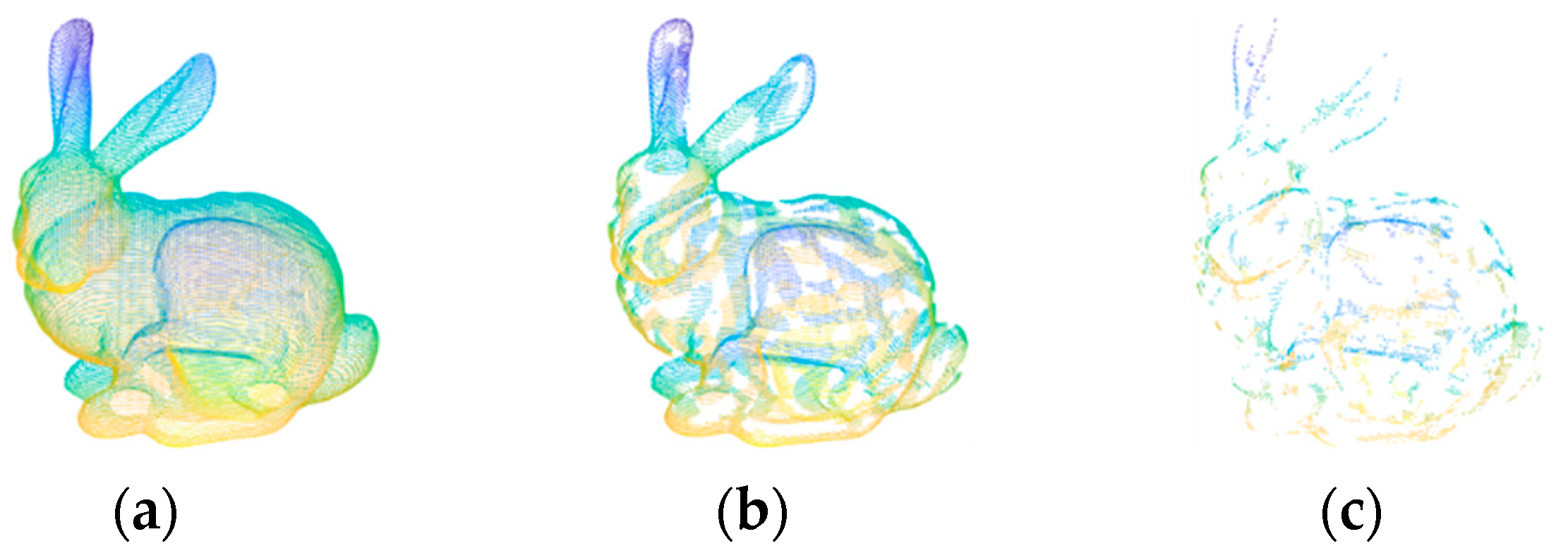
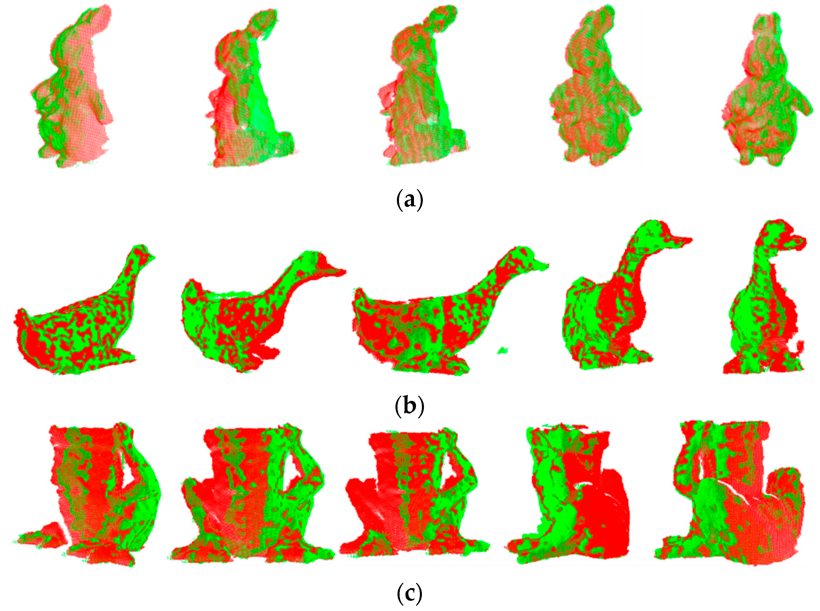
The LVS keypoint detection algorithm is primarily composed of three fundamental steps: the computation of the surface variation index, the detection of candidate keypoints, and the determination of the final keypoints. The purpose of the surface variation index is to represent local surface characteristics in a way that assigns higher values to regions with significant changes, while flat areas receive lower values. Candidate keypoint detection aims to identify points in local regions with noticeable changes, while excluding points in flat regions. The final keypoints are then derived through a simplification step aimed at reducing the number of points in changing regions, thus enhancing the quality of the final keypoints. Figure 1 illustrates the keypoint detection process, with Figure 1a originating from the B3R dataset bunny. Figure 1b displays the candidate keypoints, and Figure 1c showcases the ultimately determined keypoints.

Figure 1.
Keypoints detected by the LVS algorithm on the point cloud from the B3R dataset bunny. (a) Input point cloud, (b) candidate feature points, and (c) final feature points.
3.1.1. Computation of Surface Variation Index
For any point in the point cloud, its neighborhood point set is determined within a spherical neighborhood defined by the condition , where the search radius R is manually set. To enhance robustness against noise, the entire neighborhood point set is employed for the calculation of the covariance matrix. The covariance matrix based on is constructed as follows:
where k represents the number of points in the set and represents the centroid of . To calculate the eigenvectors and eigenvalues of the covariance matrix , Equation (3) is employed. The eigenvectors correspond to the coordinate axes of the local reference frame.
where is a diagonal matrix containing the eigenvalues of , and it satisfies . represents the matrix of eigenvectors corresponding to the eigenvalues.
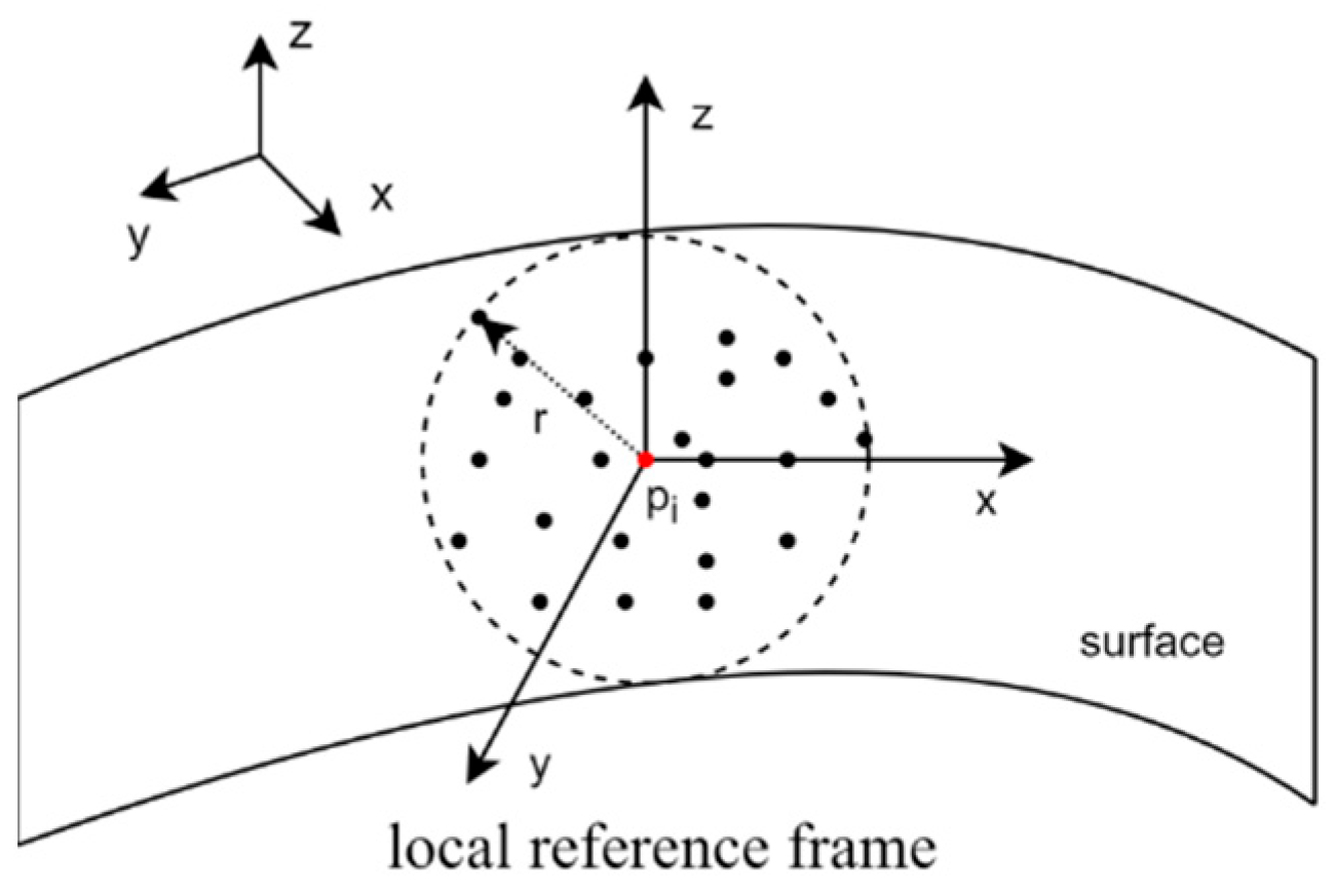
Utilizing the Hotelling transformation [16] as per Equation (4), the points in are transformed into a local reference frame formed by the three eigenvectors, as shown in Figure 2. The new neighborhood point set can be denoted as .
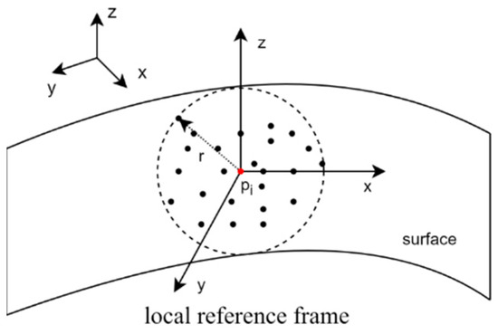
Figure 2.
Local reference frame (LRF) of the keypoint. The red dot represents the keypoint.
We define and to represent the components of the points in along the axis and axis, respectively.
We selected the absolute value ratio of the point distribution distances along the and axes, which achieved the best results through the experimental comparison of three different surface variation indices to calculate the surface variation index for point . is calculated as
3.1.2. Detection of Candidate Keypoints
As illustrated in Figure 3, the projection distribution of local neighborhood points on the plane reflects the local surface geometric changes of the point. denotes the extent of local surface geometric changes. In flat regions, the value of tends towards infinity, while in salient regions, it gradually approaches one. For feature-rich regions, the value of must be greater than one. It is important to note that setting the value of too small would result in an excessive concentration of keypoints in areas with drastic surface changes, whereas setting it too large would lead to the detection of an excessive number of keypoints. To effectively detect keypoints in different regions, the average surface variation index of point p serves as the threshold for keypoint detection. The average surface variation index is defined as follows:
where represents the surface variation index of the neighborhood points of point .
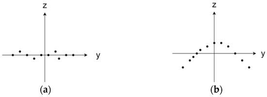
Figure 3.
The Y–Z plane projection distribution of local neighborhood points. (a) Plane region , (b) salient region .
To select local surface salient areas as feature regions, the points for which the surface variation index at point p is less than the average surface variation index are defined as follows:
Points that satisfy Equation (9) are called candidate keypoints.
3.1.3. Determination of Final Keypoint
As there may be an excessive number of candidate keypoints that meet the specified conditions, and as some of these points may not adequately represent the characteristics of the region, additional refinement of the candidate keypoints is necessary. Therefore, within the candidate keypoint set, for any point , an approach is employed to select the final keypoint. Within a neighborhood of radius surrounding the candidate keypoint, the point with the minimum value of is considered as the final keypoint. It is worth noting that the method is similar to non-maximum suppression (NMS). However, in comparison to NMS, our criteria are more permissive. To be specific, while searching for local minima within each neighborhood, we retain non-minimum points within each neighborhood rather than discarding them. The conditions for determining keypoints can be expressed as follows:
where represents a keypoint, and represents the surface variation indices of the candidate keypoints within a radius . The pseudocode summarizing the detection steps of the proposed method is outlined in Algorithm 1.
| Algorithm 1 LVS keypoint detection algorithm | |
| Input: Point Cloud | |
| Output: Keypoints | |
| 1: | procedure surface variation Index Value Estimation |
| 2: | for every point do |
| 3: | Calculate Neigh Covariance Matrix |
| 4: | Convert neighborhood points to a new coordinate system |
| 5: | Calculate Surface variation Index Value |
| 6: | return |
| 7: | procedure Candidate Keypoint Detection |
| 8: | for every point do |
| 9: | Calculate Neigh mean surface variation Index Value |
| 10: | if |
| 11: | Candidate Keypoint |
| 12: | return Candidate Keypoint |
| 13: | procedure Final Keypoint Determination |
| 14: | for every point do |
| 15: | get Nearest Neighbours |
| 16: | if |
| 17: | Keypoints |
| 18: | Return Keypoints |
3.2. Coarse-to-Fine Point Cloud Registration
Based on the proposed LVS keypoint detection algorithm, a coarse-to-fine point cloud registration method has been developed. It mainly consists of three parts: LVS keypoint detection and description, efficient SAC-GC transformation estimation, and fine registration.
3.2.1. Local Variation of Service Keypoint Detection and Description
Using and to represent the input source and target point clouds, first, the proposed LVS keypoint detection algorithm is used to detect keypoints, denoted as and , respectively. Furthermore, it is essential to describe the neighborhood information of keypoints, since the keypoints detected may contain errors due to noise or originate from different source point clouds. Descriptors, on the other hand, represent abstract structural attributes of keypoints, encapsulating more information and being less susceptible to coordinate transformations. They play a crucial role in distinguishing between different keypoints and enhancing the accuracy of the registration process. For robustness, the SHOT descriptor is used to describe and , resulting in the feature vectors and .
3.2.2. Transformation Estimation via the Sampling Consensus Correspondence Estimation Algorithm (SAC-GC)
Once the SHOT features have been computed, the next step is to establish correspondences between the feature vectors. A common approach is to select the nearest point features as corresponding point pairs. However, it is important to note that source and target point clouds often have overlapping regions only in part, which implies that correspondences exist only for some features. It is necessary to filter out non-matching keypoint pairs as
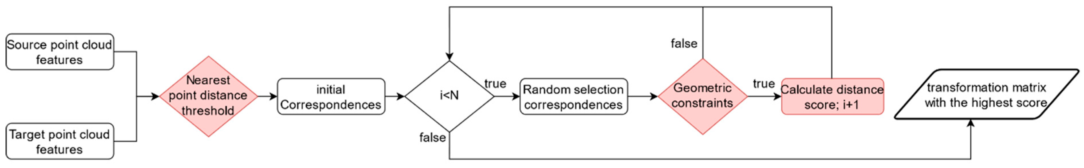
Among these pairs , , those feature vectors that satisfy the threshold criteria are considered as corresponding point pairs . All point pairs that satisfy the threshold are collectively referred to as the initial correspondence set . Despite using a threshold for filtering, the initial set may still contain numerous incorrect correspondences. Therefore, it is necessary to estimate the best transformation to align point cloud with point cloud from the set that includes erroneous correspondences. Common techniques include the RANSAC algorithm and its variants [4,18]. However, these methods often suffer from low computational efficiency. Hence, this paper introduces an efficient and robust transformation estimation method, known as the SAC-GC algorithm. The SAC-GC algorithm is designed to identify the best transformation within a specified number of iterations, denoted as from the initial correspondence set . Because the algorithm has randomness, too few iterations may not find a sufficiently good model, while too many iterations can increase the algorithm’s runtime. Based on our experience, takes 1000. In each iteration, three corresponding point pairs are randomly selected from this set . Since the keypoint pairs maintain Euclidean distance invariance before and after a rigid transformation, if three correctly corresponding point pairs form a triangle, the triangle in the source point cloud will be congruent to the triangle in the target point cloud, as follows:
However, owing to the presence of interference, there may be real differences between the two point clouds and the two triangles. To account for these differences, a geometric similarity discriminant function [19] is employed, to assess the geometric similarity between and . The discriminant function is as follows:
where represents the similarity threshold. If the corresponding point pairs satisfy the constraint in Equation (14), the transformation matrix (containing the rotation matrix and translation matrix ) is computed to align point cloud P with point cloud .
Subsequently, the traditional RANSAC method evaluates the quality of through statistics of inlier count or nearest neighbor count. However, the inlier count-based method may not accurately estimate the correct transformation, when contains a large number of erroneous information. On the other hand, the nearest neighbor count-based method requires the computation of the nearest neighbors in each iteration, which leads to higher computational complexity. In this study, we use the distance score between the corresponding points as the criteria for selecting inliers. This distance score is defined as:
where , is the distance threshold, which is set to 7.5 mr, by default. This choice is based on a local feature descriptor with a support radius of 15 mr [20]. Finally, considering the high outlier rate in point cloud registration, which can lead to the failure of non-randomness and maximal condition, the iteration count is chosen as the termination criterion for the algorithm. The above steps are repeated until the iteration count exceeds the threshold N, and the transformation matrix corresponding to the maximum distance score is selected as the final rotation matrix. Figure 4 illustrates the estimation process of SAC-GC.

Figure 4.
SAC-GC estimation process.
3.2.3. Fine Registration
After applying the SAC-GC algorithm to accomplish coarse point cloud registration, the next step is to proceed with further fine registration. While coarse registration provides an initial alignment for point clouds and , a more precise registration is necessary. To achieve this, we utilize the classic iterative closest point (ICP) algorithm [21] to further refine the results. The primary concept behind the ICP algorithm is to achieve accurate registration by minimizing the distance between point clouds and . The ICP function is as follows:
4. Experimental Results and Discussion
In this section, a series of experiments were conducted to evaluate the LVS keypoint detection algorithm, including assessing relative repeatability, absolute repeatability, and computational time. Four distinct datasets were utilized in these experiments to provide a comprehensive assessment of the algorithm’s performance. Furthermore, the point cloud registration method, based on LVS keypoints, was subjected to tests to evaluate its accuracy and robustness using the BMR dataset. It is important to note that all these experiments were carried out on a computer equipped with an Intel Core i5-13600kf 3.5 GHz processor and 32 GB of RAM, sourced from Lenovo, a Chinese brand based in Changchun.
4.1. Datasets
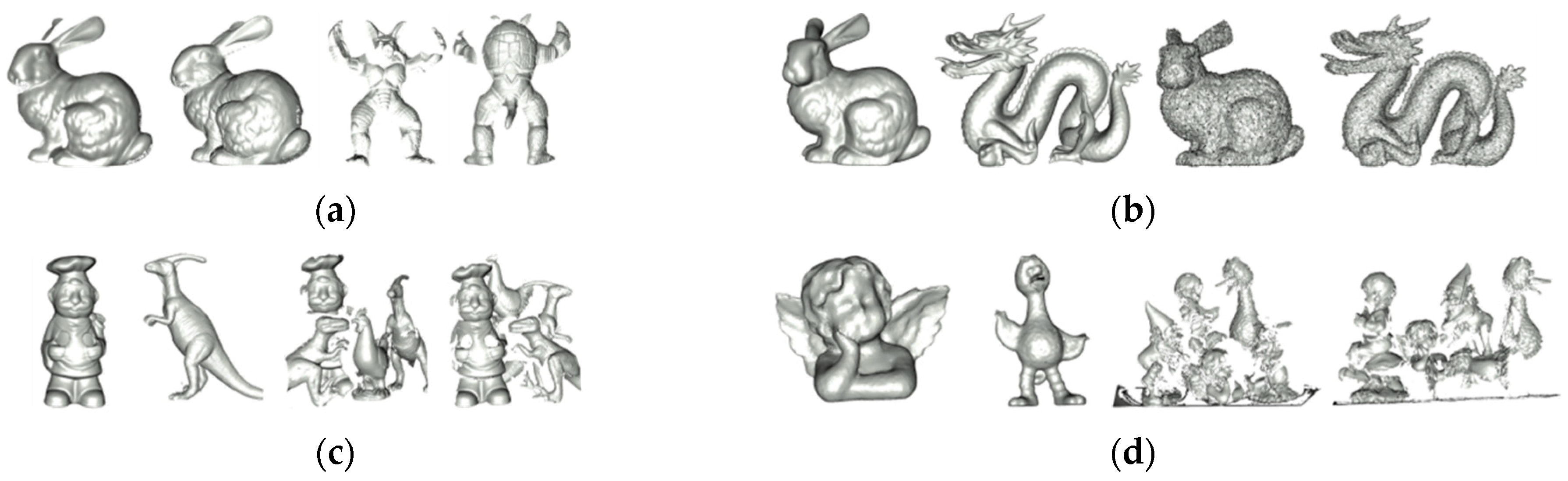
There were four datasets used to assess the performance of the proposed LVS keypoint detection method. These datasets are Stanford 3D, B3R, U3OR, and Queen. Figure 5 provides visual representations of the models and scenes within these four datasets.
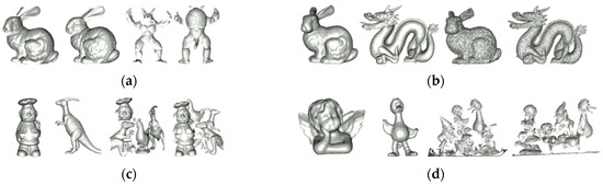
Figure 5.
Models and scenes from the Stanford 3D, B3R, U3OR, and Queen datasets. (a) Stanford 3D, (b) B3R, (c) U3OR, and (d) Queen.
The Stanford 3D dataset [22] consists of six models and their corresponding range data obtained through the Cyberware 3030 MS scanner. The point cloud data are noise-free, with a resolution of approximately 0.5 mm. The B3R dataset [23] includes six models and 18 scenes from the Stanford 3D Scanning Repository. These 18 scenes are generated by applying random transformations to the six models and adding Gaussian noise, with the values of 0.1, 0.3, and 0.5 milliradians. The data collection equipment is the same as the Stanford 3D dataset, and the data are primarily affected by rigid transformations and noise, with no occlusion. The U3OR dataset [24] comprises five models and 50 scenes. Each scene is composed of four or five models and captured using the Minolta Vivid 910 scanner with a resolution of around 0.6 mm. The data are free of noise but include occlusion and clutter. The Queen dataset [25] is composed of five models and 80 scenes, acquired using the Konica-Minolta Vivid 3D scanner. Compared to U3OR, the Queen dataset has more scene models and lower-quality data, including noise, occlusion, clutter, and resolution variations.
4.2. Parameter Analysis
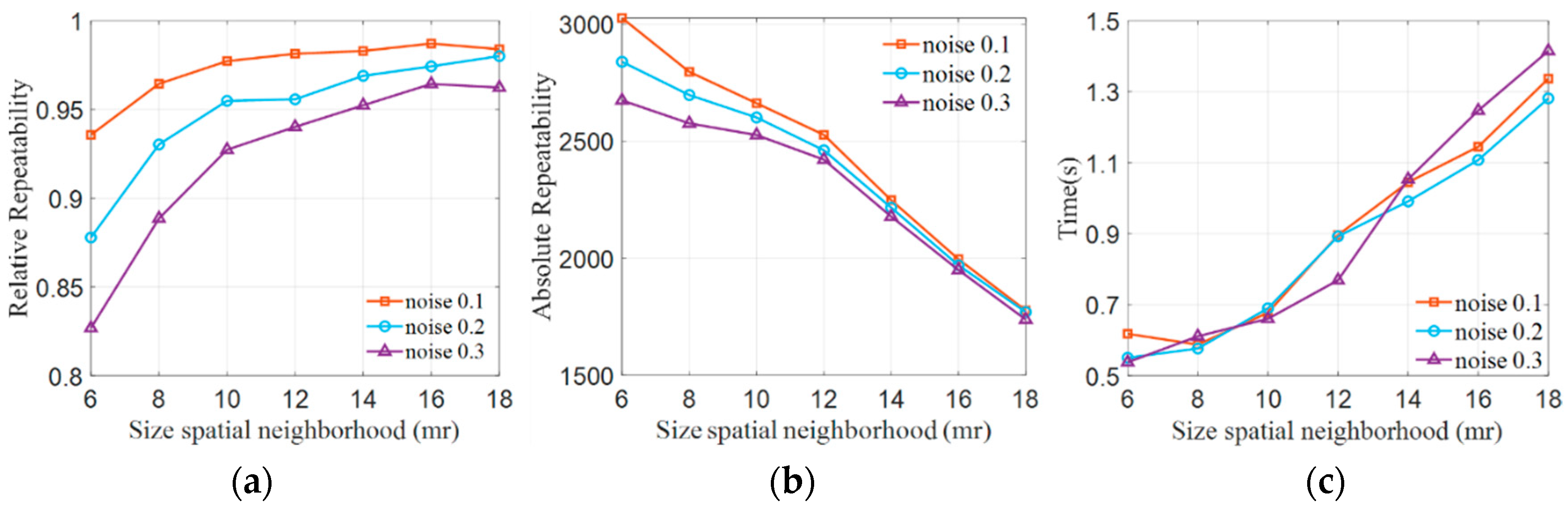
The neighborhood radius is a crucial parameter in point cloud feature detection, and its value directly influences the recognition of point cloud features. If is set too large, it increases computational complexity and diminishes robustness against occlusions and point cloud boundaries. Conversely, when is set too small, it diminishes feature distinctiveness. To better analyze the impact of the neighborhood radius on keypoint detection, a methodology similar to that in reference [6] was employed. The Stanford point cloud data were used as test data, as discussed in detail in Section 4.1, and Gaussian noise, with values of 0.1 mr, 0.2 mr, and 0.3 mr, was introduced into the test point cloud. The neighborhood radius was set at 6 mr, 8 mr, 10 mr, 12 mr, 14 mr, 16 mr, and 18 mr where mr represents the point cloud resolution, which indicates the average distance between neighboring points in the point cloud. The relative repeatability and absolute repeatability of keypoint detection were assessed separately. Relative repeatability is defined by Formula (17), while absolute repeatability is defined by Formula (18). We also evaluated the computation time. The experimental results are presented in Figure 6.
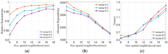
Figure 6.
Impact of different neighborhood radii on keypoints. (a) Relative repeatability, (b) absolute repeatability, and (c) computational Time.
As shown in Figure 6a, the relative repeatability of keypoints demonstrates an increase as the neighborhood radius R expands for different noise levels. When R is set at values less than 10 mr, the relative repeatability of keypoints experiences a significant uptick as the radius increases, particularly in the case of various noise point cloud data. Nevertheless, when R surpasses 10 mr, the relative repeatability of keypoints registers a more gradual increase with the expanding radius. In Figure 6b, the absolute repeatability of keypoints follows a consistent pattern, decreasing linearly as the neighborhood radius grows across different noise levels. This outcome is attributed to the increasing radius, leading to the detection of more stable features while filtering out lower-quality keypoints. In Figure 6c, it is shown that the growth is slow for R values less than 10 mr, and then it increases rapidly. Consequently, it is concluded that a neighborhood radius of 10 mr is well-suited for the keypoint detection method.
4.3. Evaluation Criteria for Keypoints
All keypoint methods employ keypoint repeatability as a widely accepted evaluation criterion. Evaluation methods for keypoint repeatability can be found in the following references [6,11,18]. Keypoint repeatability pertains to the capability of a keypoint detection algorithm to consistently locate the same keypoint in the same local region of the same model. High keypoint repeatability indicates that the detection algorithm demonstrates strong resistance to interference, such as noise, occlusion, and clutter.
Keypoint repeatability is typically divided into two categories: relative repeatability and absolute repeatability. The primary calculation steps are as follows: first, keypoint sets are independently detected from the source point cloud and the target point cloud, denoted as and , respectively. Next, the keypoints detected from the source point cloud are aligned to the target point cloud using the true rotation and translation matrices, where the true rotation and translation matrix data are provided from datasets. If a keypoint in the source point cloud is at a distance less than the threshold from the nearest neighbor keypoint in the target point cloud, it is considered repeatable; that is:
Based on Equation (17), the total number of keypoints that meet the conditions detected from the source point cloud is denoted as . The definitions of absolute repeatability and relative repeatability are as follows:
where is the number of keypoints in the source point cloud.
4.4. Keypoint Repeatability Experiment
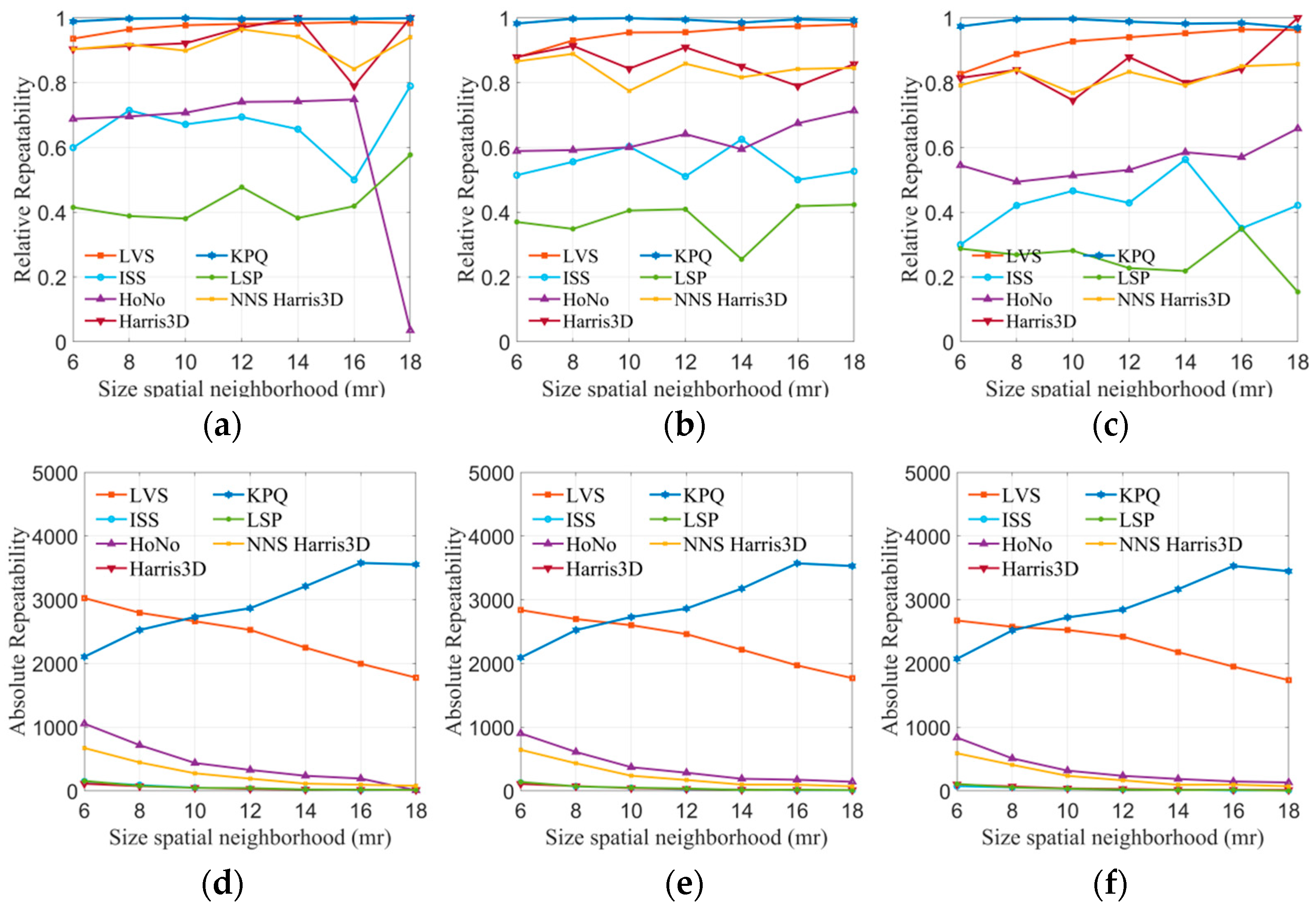
In this experiment, the LVS keypoint detection algorithm proposed in this paper was compared with six advanced methods (ISS, HoNo, Harris 3D, KPQ, LSP, NNS Harris 3D) using four public datasets. Due to errors or interference in point cloud devices, true corresponding points may exhibit a small offset. Therefore, a threshold that is too small might exclude correct corresponding points, while a threshold that is too large could result in the consideration of erroneous points. The distance threshold was set to 2 mr, where mr represented the average distance between points in the point cloud. The neighborhood radius was set to 6 mr, 8 mr, 10 mr, 12 mr, 14 mr, 16 mr, and 18 mr, respectively. The experiment calculated the relative repeatability and absolute repeatability of each algorithm under varying neighborhood radii. The results are displayed in Figure 7.
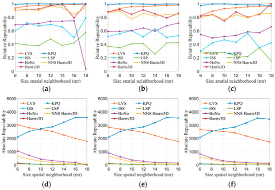
Figure 7.
The tests of absolute and relative repeatability on the B3R dataset. (a) 0.1 mr Gaussian noise, (b) 0.2 mr Gaussian noise, (c) 0.3 mr Gaussian noise, (d) 0.1 mr Gaussian noise, (e) 0.2 mr Gaussian noise, and (f) 0.3 mr Gaussian noise.
For the B3R dataset, the robustness of all methods in noisy environments was evaluated. The results of keypoint detection algorithms are presented in Figure 7a–f. Regarding keypoint repeatability (Figure 7a–c), LVS and KPQ performed exceptionally well, significantly surpassing other methods. The line graphs clearly illustrate that the LVS keypoint detection algorithm can maintain a repeatability rate of over 80% across different noise levels, and this rate increases with the radius. Harris 3D and NNS Harris 3D also demonstrated decent performance, with a repeatability rate fluctuating around 80%. However, HoNo, LSP, and ISS performed less satisfactorily, possibly due to the sensitivity of HoNo’s normal vectors, LSP’s curvature to noise, and ISS potentially containing planar points. Regarding keypoint absolute repeatability (Figure 7d–f), it is evident that, under varying noise conditions, KPQ and LVS consistently have the highest number of repeatable keypoints compared to the other methods. The number of keypoints they detect is less affected by noise. In contrast, ISS, HoNo, Harris 3D, LSP, and NNS Harris 3D detect fewer keypoints, which may be attributed to the impact of non-maximum suppression, implying that non-maximum suppression filtered out a significant portion of the keypoints.
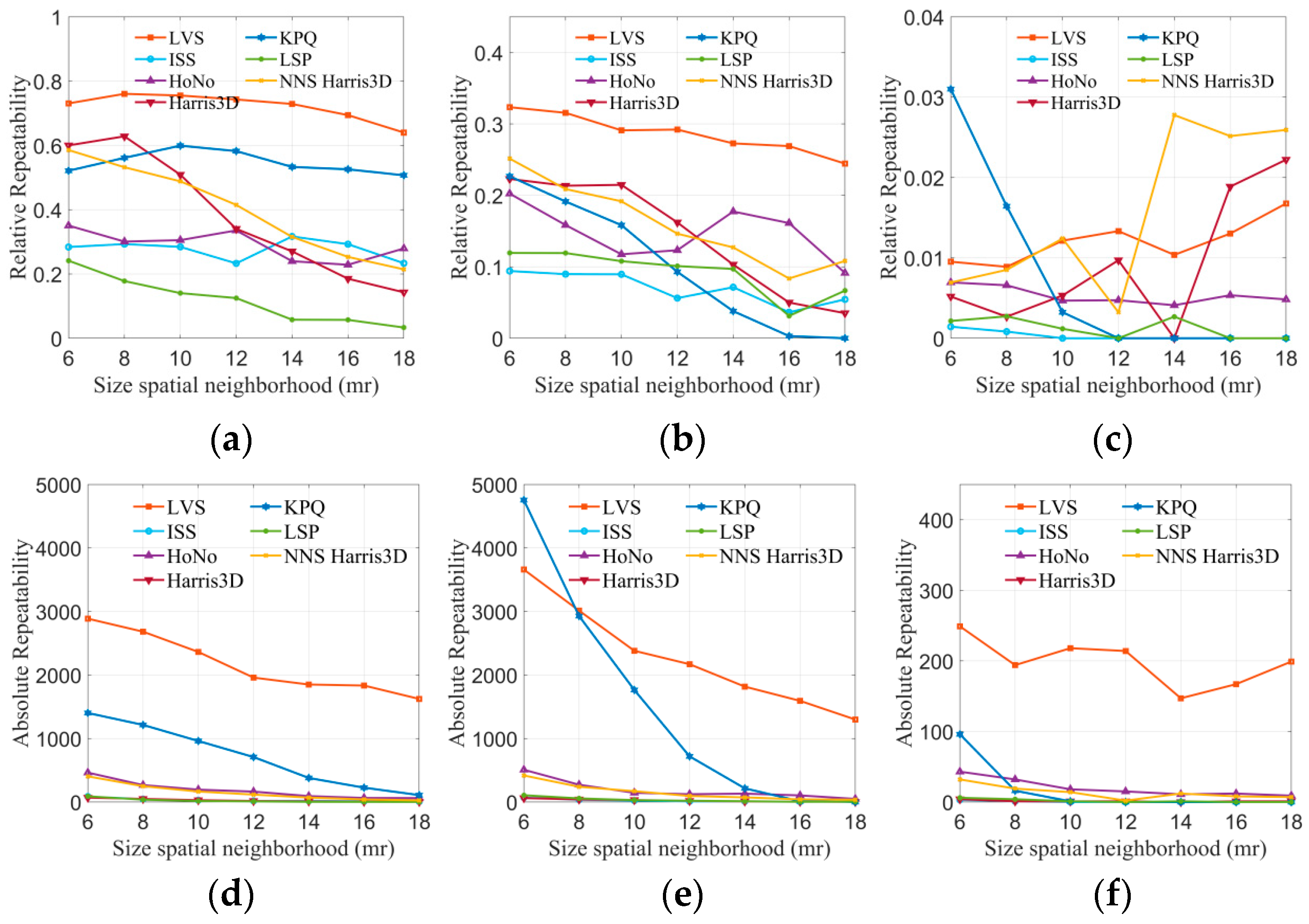
Robustness experiments were conducted for all keypoint detection algorithms under occlusion, clutter, and border conditions, using the Stanford 3D and U3OR datasets. The results are presented in Figure 8, where (a, b) represent relative repeatability. It is evident from the graphs that LVS outperforms all other algorithms on both datasets. In Figure 8d,e depicting absolute repeatability, it can be observed that as the radius increases, the number of repeatable points gradually decreases for all algorithms. However, LVS consistently maintains 1000 or more repeatable points at various radii, while the other methods gradually tend to zero. This demonstrates the robustness of LVS against occlusion, clutter, and border conditions. The robustness of LVS can be attributed to two key factors: firstly, LVS detects keypoints based on the average surface change index, eliminating points in flat regions and enhancing the quality of keypoints by filtering out redundant points.
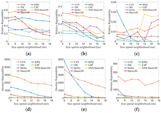
Figure 8.
The tests of absolute and relative repeatability on the Stanford 3D, U3OR, and Queen datasets. (a) Stanford 3D, (b) U3OR, (c) Queen, (d) Stanford 3D, (e) U3OR, and (f) Queen.
The Queen dataset, being of lower quality than the others, presents significant challenges due to its higher noise level, complex background, and sparse point distribution. The results of the seven methods are presented in Figure 8c,f. Regarding relative repeatability, KPQ and NNS Harris 3D exhibit the largest fluctuations, while LVS remains relatively stable. Furthermore, the absolute repeatability of LVS surpasses that of the other methods, providing a substantial number of keypoints for subsequent registration. This underscores the robustness of the LVS keypoint detection algorithm in handling various interferences.
4.5. Keypoint Computation Efficiency
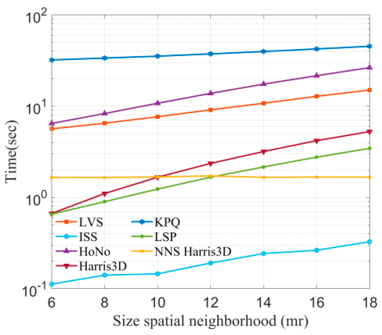
In this section, the efficiency of all methods will be compared. Since the efficiency of the keypoint computation is related to the number of points in the original point cloud, this study selected the B3R dataset for testing. Radii are set from 6 mr to 18 mr, with a 2 mr interval, and then seven keypoint detection algorithms are used to detect keypoints at different radii. The results of time consumption are shown in Figure 9.

Figure 9.
Time consumption of keypoint detection algorithms at different radii.
We can observe that ISS is the most efficient method, since it only requires the computation of eigenvalue ratios. Secondly, KPQ is the most time-consuming, as it needs to perform surface fitting to compute keypoint quality. It is worth noting that LVS employs a method similar to KPQ but is more efficient relative to KPQ and HoNo.
4.6. Registration Algorithm Comparison Experiment
In this section, the proposed registration algorithm based on LVS is evaluated. The evaluation experiments include qualitative and quantitative analyses, as well as comparisons with state-of-the-art algorithms. These experiments use the BMR dataset, which comprises point clouds obtained from various viewpoints using a Microsoft Kinect device. The point clouds in this dataset are challenging, and are characterized by noise, occlusions, missing data, and variations in resolution. Therefore, this dataset provides a comprehensive assessment of the registration algorithm’s performance. The registration parameters for the algorithm are set based on the analysis in Section 4.2, with = 10 mr, , , .
4.7. Qualitative Results
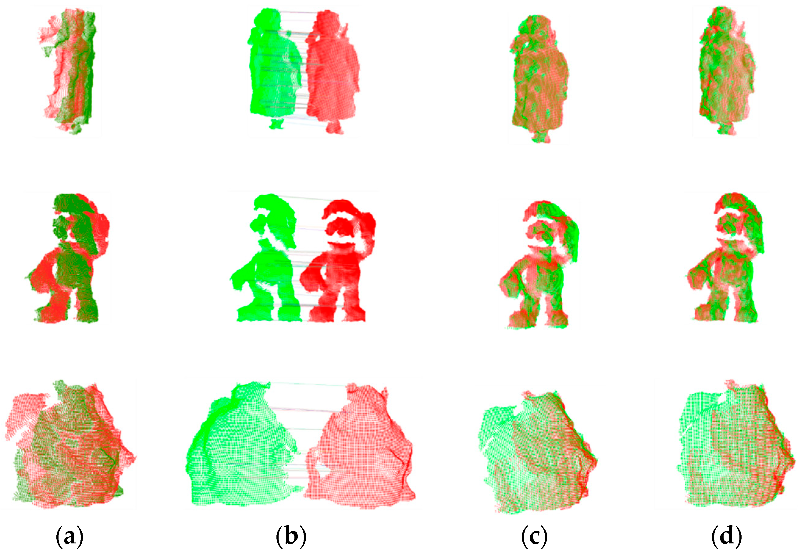
Figure 10 displays the registration results of the proposed method for point clouds with varying angles and overlap ratios. The original point clouds pose challenges such as holes, missing data, and occlusions, which can make registration a challenging task.
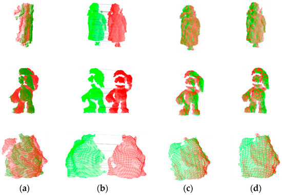
Figure 10.
The point cloud registration effect. (a) Initial, (b) correspondences, (c) coarse, and (d) fine.
However, our registration method can establish partially accurate correspondences and compute initial poses, providing a good starting point for fine registration. This reflects the ability of the proposed LVS keypoint detection method to identify a significant number of repeatable keypoints and underscores the robustness of LVS features to various interferences. It is worth noting that our algorithm is fully automatic and requires only the input of source and target point clouds to produce registration results. To validate the effectiveness of the algorithm, we also present 15 registration results in Figure 11.

Figure 11.
Registration results of the LVS-based registration algorithm for BMR set. (a) PeterRabbit, (b) Duck, and (c) Frog.
4.8. Quantitative Results
In addition to the visual analysis, we conducted quantitative analyses of the registration results, including the time required for registration, rotation error, and translation error.
To measure the accuracy of registration, rotation error and translation error were used. Rotation error is between the estimated and the true rotation matrix, while translation error is between the estimated and the true translation vector. Specifically, they are defined as follows:
where and are the results obtained through manual initial alignment and refined using ICP registration.
To further validate the superiority of our proposed registration algorithm, we conducted a comparison of registration errors between our method and other methods. To ensure a fair comparison, we utilized the same registration pipeline, and the various methods only replaced the keypoint detection algorithms. We estimated the initial pose using SAC-GC and the final pose using ICP. Subsequently, we compared the performance of different methods at 80% and 50% overlap rates, with the calculation of overlap rates following the reference [4]. Table 1 presents all the registration results.

Table 1.
Comparison of our LVS-based registration algorithm with six state-of-the-art methods (the top two results are in bold).
As indicated in Table 1, all methods exhibit notable errors in the fine registration results, primarily due to the substantial interference in the BMR dataset, which poses challenges in initial pose estimation. Nevertheless, the LVS-based registration method consistently achieves the lowest rotation and translation errors across all datasets. The KPQ method, which detects fewer keypoints, performs the least effectively. At an 80% overlap rate, both LVS and the method based on NNS Harris 3D outperform the other methods in all datasets. The remaining methods exhibit optimal performance in only a few datasets. As the overlap rate decreases to 50%, registration becomes more challenging, leading to increased errors for all registration methods. The methods based on HoNo, Harris 3D, KPQ, LSP, and NNS Harris 3D display significant rotation and translation errors across all datasets as they struggle to detect repeatable keypoints. The ISS-based method performs reasonably well only on the Frog dataset.
To validate the improvement in SAC-GC over RANSAC, tests were conducted by replacing SAC-GC with RANSAC while maintaining the same number of iterations. The summarized experimental results are presented in the table below. It is evident from Table 2 that each method has its strengths and weaknesses in terms of rotation and translation errors. Notably, SAC-GC offers a 14-fold speedup over RANSAC, due to the geometric similarity filtering, which eliminates a substantial number of incorrect point pairs.
Table 2.
Performance of SAC-GC and RANSAC in terms of rotation and translation errors, and computational times.
5. Conclusions
This paper introduces a keypoint detection algorithm and a registration algorithm based on LVS. The LVS keypoint detection method begins by computing a local coordinate system for each point in the point cloud. In this local coordinate system, a surface variation index is calculated based on the coordinate axis ratios. Points with surface variation indices smaller than the local average value are identified as candidate keypoints. Subsequently, the point with the smallest surface variation index in the neighborhood of each candidate keypoint is selected as the final keypoint. Based on LVS keypoints, an efficient and accurate registration algorithm is proposed.
Extensive experimental evaluations were conducted to assess the performance of the proposed keypoint detector and registration algorithm. For keypoint evaluation, tests were conducted on four datasets, which contained noise, clutter, occlusion, and resolution variations. Compared to existing keypoint detectors, the LVS keypoint detector exhibited higher keypoint repeatability. The results also demonstrated the efficiency of the LVS detector. In the context of registration, experiments were carried out on low-quality point cloud datasets using the LVS and SAC-GC registration method. Qualitative and quantitative results demonstrated outstanding performance in terms of accuracy and efficiency. This was primarily attributed to the high repeatability of LVS keypoints and the efficient change estimation of the SAC-GC algorithm. Moreover, a comparison between SAC-GC and RANSAC under the same performance conditions revealed a 14-fold increase in efficiency for SAC-GC.
Author Contributions
Conceptualization, J.Z. and Z.H.; methodology, Z.H.; software, Z.H.; validation, Z.H. and Z.L.; formal analysis, J.Z. and X.Y.; investigation, Z.H.; resources, J.Z.; data curation, Z.L.; writing—original draft preparation, Z.H.; writing—review and editing, J.Z. and Z.L.; visualization, Z.H.; and supervision, J.Z. and X.Y. All authors have read and agreed to the published version of the manuscript.
Funding
The authors acknowledge the Department of Science and Technology of Jilin province (20220203091SF).
Data Availability Statement
The datasets used and/or analyzed during the current study are available from the corresponding author on reasonable request.
Conflicts of Interest
The authors have no relevant financial or non-financial interest to disclose.
References
- Liu, Y.; Kong, D.; Zhao, D.; Gong, X.; Han, G. A Point Cloud Registration Algorithm Based on Feature Extraction and Matching. Math. Probl. Eng. 2018, 2018, 7352691. [Google Scholar] [CrossRef]
- Feng, H.; Ren, X.; Li, L.; Zhang, X.; Chen, H.; Chai, Z.; Chen, X. A novel feature-guided trajectory generation method based on point cloud for robotic grinding of freeform welds. Int. J. Adv. Manuf. Technol. 2021, 115, 1763–1781. [Google Scholar] [CrossRef]
- Kim, P.; Park, J.; Cho, Y.K.; Kang, J. UAV-assisted autonomous mobile robot navigation for as-is 3D data collection and registration in cluttered environments. Autom. Constr. 2019, 106, 102918. [Google Scholar] [CrossRef]
- Quan, S.; Ma, J.; Hu, F.; Fang, B.; Ma, T. Local voxelized structure for 3D binary feature representation and robust registration of point clouds from low-cost sensors. Inf. Sci. 2018, 444, 153–171. [Google Scholar] [CrossRef]
- Liu, X.; Li, A.; Sun, J.; Lu, Z. Trigonometric projection statistics histograms for 3D local feature representation and shape description. Pattern Recognit. 2023, 143, 109727. [Google Scholar] [CrossRef]
- Tombari, F.; Salti, S.; Di Stefano, L. Performance Evaluation of 3D Keypoint Detectors. Int. J. Comput. Vis. 2013, 102, 198–220. [Google Scholar] [CrossRef]
- Zhong, Y. Intrinsic shape signatures: A shape descriptor for 3D object recognition. In Proceedings of the IEEE 12th International Conference on Computer Vision Workshops, ICCV Workshops, Kyoto, Japan, 27 September–4 October 2009; pp. 689–696. [Google Scholar]
- Sipiran, I.; Bustos, B. Harris 3D: A robust extension of the Harris operator for interest point detection on 3D meshes. Vis. Comput. 2011, 27, 963–976. [Google Scholar] [CrossRef]
- Mian, A.; Bennamoun, M.; Owens, R. On the Repeatability and Quality of Keypoints for Local Feature-based 3D Object Retrieval from Cluttered Scenes. Int. J. Comput. Vis. 2010, 89, 348–361. [Google Scholar] [CrossRef]
- Iqbal, M.Z.; Bobkov, D.; Steinbach, E. Fuzzy logic and histogram of normal orientation-based 3D keypoint detection for point clouds. Pattern Recognit. Lett. 2020, 136, 40–47. [Google Scholar] [CrossRef]
- Yue, X.; Liu, Z.; Zhu, J.; Gao, X.; Yang, B.; Tian, Y. Coarse-fine point cloud registration based on local point-pair features and the iterative closest point algorithm. Appl. Intell. 2022, 52, 12569–12583. [Google Scholar] [CrossRef]
- Wang, Y.; Zhou, T.; Li, H.; Tu, W.; Xi, J.; Liao, L. Laser point cloud registration method based on iterative closest point improved by Gaussian mixture model considering corner features. Int. J. Remote Sens. 2022, 43, 932–960. [Google Scholar] [CrossRef]
- Chen, H.; Bhanu, B. 3D free-form object recognition in range images using local surface patches. Pattern Recognit. Lett. 2007, 28, 1252–1262. [Google Scholar] [CrossRef]
- Zeng, H.; Wang, H.; Dong, J. Robust 3D keypoint detection method based on double Gaussian weighted dissimilarity measure. Multimed Tools Appl. 2017, 76, 26377–26389. [Google Scholar] [CrossRef]
- Lan, J.; Wang, Z.; Li, J.; Yuan, M.; Gao, X. Keypoint Extraction Algorithm Based on Normal Shape Index. Laser Optoelectron. Prog. 2020, 57, 161016. [Google Scholar] [CrossRef]
- Fengguang, X.; Xie, H. A 3D Surface Matching Method Using Keypoint- Based Covariance Matrix Descriptors. IEEE Access 2017, 5, 14204–14220. [Google Scholar] [CrossRef]
- Prakhya, S.M.; Liu, B.; Lin, W. Detecting keypoint sets on 3D point clouds via Histogram of Normal Orientations. Pattern Recognit. Lett. 2016, 83, 42–48. [Google Scholar] [CrossRef]
- Yang, J.; Zhang, Q.; Cao, Z. Multi-attribute statistics histograms for accurate and robust pairwise registration of range images. Neurocomputing 2017, 251, 54–67. [Google Scholar] [CrossRef]
- Zou, X.; He, H.; Wu, Y.; Chen, Y.; Xu, M. Automatic 3D point cloud registration algorithm based on triangle similarity ratio consistency. IET Image Process. 2020, 14, 3314–3323. [Google Scholar] [CrossRef]
- Yang, J.; Huang, Z.; Quan, S.; Zhang, Q.; Zhanga, Y.; Cao, Z. Toward Efficient and Robust Metrics for RANSAC Hypotheses and 3D Rigid Registration. IEEE Trans. Circuits Syst. Video Technol. 2021, 32, 893–906. [Google Scholar] [CrossRef]
- Besl, P.J.; McKay, N.D. A Method for Registration of 3-D Shapes. IEEE Trans. Pattern Anal. Mach. Intell. 1992, 14, 239–256. [Google Scholar] [CrossRef]
- Yan, Z.; Wang, H.; Liu, X.; Ning, Q.; Lu, Y. Binary Feature Description of 3D Point Cloud Based on Retina-like Sampling on Projection Planes. Machines 2022, 10, 984. [Google Scholar] [CrossRef]
- Yang, J.; Fan, S.; Huang, Z.; Quan, S.; Wang, W.; Zhang, Y. VOID: 3D object recognition based on voxelization in invariant distance space. Vis. Comput. 2022, 39, 3073–3089. [Google Scholar] [CrossRef]
- Zhao, B.; Yue, J.; Tang, Z.; Chen, X.; Fang, X.; Le, X. A Novel Local Feature Descriptor and an Accurate Transformation Estimation Method for 3-D Point Cloud Registration. IEEE Trans. Instrum. Meas. 2023, 72, 1–15. [Google Scholar] [CrossRef]
- Zhao, H.; Tang, M.; Ding, H. HoPPF: A novel local surface descriptor for 3D object recognition. Pattern Recognit. 2020, 103, 107272. [Google Scholar] [CrossRef]

Disclaimer/Publisher’s Note: The statements, opinions and data contained in all publications are solely those of the individual author(s) and contributor(s) and not of MDPI and/or the editor(s). MDPI and/or the editor(s) disclaim responsibility for any injury to people or property resulting from any ideas, methods, instructions or products referred to in the content. |
© 2023 by the authors. Licensee MDPI, Basel, Switzerland. This article is an open access article distributed under the terms and conditions of the Creative Commons Attribution (CC BY) license (https://creativecommons.org/licenses/by/4.0/).