A Spatiotemporal Graph Neural Network with Graph Adaptive and Attention Mechanisms for Traffic Flow Prediction

Abstract

This study addresses the complex challenges associated with road traffic flow prediction and congestion management through the enhancement of the attention-based spatiotemporal graph convolutional network (ASTGCN) algorithm. Leveraging toll data and real-time traffic flow information from Orange County, California, the algorithm undergoes refinement to adeptly capture abrupt changes in road traffic dynamics and identify instances of acute congestion. The optimization of the graph structure is approached from both macro and micro perspectives, incorporating key factors such as road toll information, node connectivity, and spatial distances. A novel graph self-learning module is introduced to facilitate real-time adjustments, while an attention mechanism is seamlessly integrated into the spatiotemporal graph convolution module. The resultant model, termed AASTGNet, exhibits superior predictive accuracy compared to existing methodologies, with MAE, RMSE, and MAPE values of 8.6204, 14.0779, and 0.2402, respectively. This study emphasizes the importance of incorporating tolling schemes in road traffic flow prediction, addresses static graph structure limitations, and adapts dynamically to temporal variations and unexpected road events. The findings contribute to advancing the field of traffic prediction and congestion management, providing valuable insights for future research and practical applications.

1. Introduction

Presently, in economically developed regions, the growth in user demand for transportation services exceeds the capacity expansion in road infrastructure supply. This imbalance has given rise to an increasingly severe issue of traffic congestion. In tackling recurrent road traffic congestion, the application of congestion tolling represents a viable approach to alleviate this challenge [1,2,3,4,5,6,7,8,9,10,11,12]. Conversely, for the effective management of unforeseen road traffic congestion, a pivotal requirement lies in the capability to discern instances and locations of sudden congestion through rigorous scientific methodologies [13,14]. Both knowledge-driven and data-driven methodologies can be employed to address this complex issue [15,16,17,18,19,20,21]. Drawing upon traffic flow theory, knowledge-driven algorithms are developed to establish models for the dissipation of congestion [14]. These models deduce information about congested nodes, queue lengths, and the times required for congestion dissipation, utilizing insights derived from transient changes in road service levels resulting from unforeseen circumstances. Knowledge-driven methodologies encompass a myriad of theoretical assumptions, giving rise to specific divergences between anticipated outcomes and real-world scenarios. With the advancement of artificial intelligence, employing data-driven methods to analyze abrupt changes in road traffic volume and infer the location and timing of congestion occurrences is a preferable choice, which shares similarities with data-driven road traffic flow prediction tasks [22]. Both tasks involve making judgments about the future road traffic state based on real-time data collected from the current road conditions. Traffic flow prediction tasks primarily focus on inferring the future road traffic volume over a specific time period, while the diagnostic task for sudden road traffic congestion emphasizes capturing the abrupt changes in road traffic flow. The field of road traffic flow prediction has evolved over several decades, providing an opportunity to transfer the research achievements in this domain toward the direction of sudden congestion identification. Detecting sudden changes in road traffic flow can significantly address the issue of predicting unexpected road traffic congestion.

The evolution of road traffic flow prediction tasks can be delineated into three stages: employing time series methods, adopting machine learning methodologies, and embracing deep learning approaches. Time series methods primarily encompass the historical average model [23], the auto-regressive integrated moving average [24], and the vector autoregressive model [25]. Time series methods rely on data exhibiting relatively strong stationarity; however, traffic flow data typically demonstrate pronounced seasonality and periodicity. Hence, machine learning and deep learning methods remain unaffected by stationarity and can model the intricate non-linear relationships within road traffic flow. Methods such as k-nearest neighbors (KNNs) [26], support vector regression (SVR) [27], recurrent neural networks (RNNs) [28], convolutional neural networks (CNNs) [29], and graph neural networks (GNNs) [30] have been proposed for application in this domain. Davis et al. [31] indicated that the traditional KNN did not exhibit significant enhancement compared with the time series methods. Jeong et al. [32] proposed an enhanced SVR algorithm for short-term road traffic flow prediction. However, the algorithm exhibits a strong dependence on data from the nearest time points and does not account for the mutual influences between adjacent nodes. As a remedy, the CNN and RNN were used to extract the correlation of data in the temporal dimension, and the KNN, CNN, and GNN were used to the correlation of data in the spatial dimension. Luo et al. [33] employed LSTM and the KNN to, respectively, capture the temporal and spatial features of traffic flow. In the context of spatial traffic information, the KNN can only identify the most relevant traffic stations. Yao et al. [34] employed a CNN to extract spatial relationships within the data and LSTM to capture temporal relationships. However, a comprehensive explanation for the efficacy of a CNN was not provided. GNNs are better suited for handling non-Euclidean spatial relationships among road sensors. Li et al. [35] used a GNN combined with an RNN to deal with the complexity of traffic data in time-space. Guo et al. [36] used a GNN combined with a CNN accompanied by an attention mechanism to process traffic data for road traffic flow prediction. Long et al. [37] proposed USTAN, a unified spatiotemporal attention network, which addresses challenges by employing a unified attention component and a gated fusion module for adaptive external factor modeling, demonstrating outstanding performance in practical tasks.

The road traffic flow prediction algorithm based on graph neural networks is currently a high-precision, data-driven, and short-term traffic flow forecasting method. However, it has two main shortcomings. Firstly, the generation of the road traffic graph structure relies primarily on prior theoretical knowledge, which may not adequately reflect the connectivity between nodes. If the relationship between nodes relies on the distance of the nodes, this relationship will deviate significantly from the actual situation, as shown in Figure 1. In Figure 1, while the distance between areas B and C appears short, there is a diversion area between them that may weaken their connection relative to the connection between A and B. Similarly, the presence of a toll station between C and D can significantly affect the relationship between them, with this influence manifesting at both static or macro-levels and dynamic or micro-levels. Zhang et al. [38] addressed this issue by proposing a self-learning graph structure that leverages multiple sources of prior knowledge as the starting point for graph structure self-learning. During the model training process, they performed alternating iterative optimization of graph structure parameters and traffic flow prediction model parameters based on the loss function. The judicious selection of prior knowledge holds significant importance in the process of self-learning for graphs. Inappropriately chosen prior knowledge may lead the model into inappropriate local optima during self-learning, constraining the ultimate precision achievable by the model. Given the context of employing a time-based tolling strategy for the proactive regulation of recurrent road traffic congestion, incorporating the tolling strategy as prior knowledge in the self-learning graph is anticipated to enhance the model’s training effectiveness. The second issue lies in the static nature of the graph structure of the road traffic network, which fails to adapt dynamically to temporal changes and respond effectively to unforeseen events on the roads. Figure 2 further illustrates how the relationship between areas can be influenced by various factors and can change over time. In Figure 2a, it is evident that the interregional traffic relationships are subject to the influence of changes in toll collection status, whereby the price change of toll collection at specific road sections may alter traffic flows and, consequently, impact traffic relationships. In Figure 2b, the time-varying nature of traffic relationships is demonstrated, whereby the relationships between areas can be modified by traffic management policies, such as road repair or road closures. Finally, Figure 2c shows how traffic congestion or road construction can affect the relationships between areas over time, leading to changes in traffic patterns and potentially altering the dynamics of traffic flow. To address this concern, Ta et al. [39] proposed a solution by introducing a micro-level self-learning graph structure. This approach involves real-time adjustments to the graph structure based on the fluctuations in node traffic flow, thereby enhancing the model’s ability to accommodate temporal variations and promptly react to unexpected road conditions. Additionally, with regard to the road traffic flow prediction module of the graph neural network, in the context of employing tolling schemes to regulate recurrent road traffic congestion, the current tolling policies on the roads can significantly influence the travel strategies adopted by users. Therefore, in the process of road traffic flow prediction, due consideration should be given to the impact of the prevailing congestion pricing schemes on the road traffic volume.

To address these issues, this study enhances the road traffic flow prediction algorithm based on attention-based spatiotemporal graph convolutional networks (ASTGCNs) using toll data and real-time traffic flow data from Orange County, California, USA. The primary focus is on refining the algorithm to effectively capture sudden changes in road traffic flow and diagnose instances of acute road traffic congestion. For the graph structure, optimization is conducted from both macro and micro perspectives. At the macro level, road toll information, connectivity between nodes, and the spatial distances among nodes are utilized as prior knowledge to construct an initial graph structure. During the model training process, synchronous optimization is applied to the macro-level graph structure. On the micro level, the current moment’s micro-level graph structure is generated using node traffic flow data. It is then concatenated with the macro-level graph structure, enabling real-time optimization of the graph structure. In the traffic flow prediction model module, a spatiotemporal graph convolution module, incorporating an attention mechanism, is employed to forecast road traffic flow for a future time horizon. Building on this, the current service level of the road is assessed based on the present road capacity. The algorithm comprises a graph self-learning module, a time-attention module, and a spatiotemporal graph convolutional neural network module, collectively referred to as a spatiotemporal graph neural network with graph adaptive and attention mechanisms (AASTGNet).

2. Methods

2.1. Initial Graph Structure

The efficacy of convolutional operations is directly influenced by the quality of the graph structure. To enhance the quality of the graph structure and mitigate the risk of the model prematurely converging to inappropriate local optima during iterative training, three pre-defined graph structures are introduced in this section. These include the node connectivity graph structure, the distance graph structure, and the toll graph structure.

2.1.1. Node Connectivity Graph Structure

The node connectivity graph structure specifically refers to the physical connectivity between detectors in the real world by connecting node sensors in both directions in which traffic could flow. The connections between detectors in freeway junction areas are of particular importance. In this study, the two junction areas between SR241 and SR261, and SR241 and SR133, were considered. Figure 3 depicts the spatial position information and connection relations of the detectors, with the key nodes in (a) and (b) being numbered and their connections are described in the figure.

2.1.2. Distance Graph Structure

The distance graph structure refers to the spatial distance between node detectors, regardless of their actual connection in the real world. Unlike the node connectivity graph structure, the distance graph structure also includes nodes that are not directly connected but are located close to each other in space. The purpose of including such nodes is to enable the model to capture the potential spatial relationship between nodes, which can enhance its performance in analyzing the traffic flow and toll data. For distances between node sensors $S_i$ and $S_j$, normalization was performed using the Gaussian kernel weighting function [40].

$$A_2^{\left(i,j\right)}=\left\{\begin{array}{l}\exp \left(-\frac{{\left|dist\left(i,j\right)\right|}^2}{2{\theta }^2}\right) \mathrm{if} dist\left(i,j\right)\le \mathrm{T}\\ 0\hspace{1em}\hspace{1em}\hspace{1em}\hspace{1em}\hspace{1em}\hspace{1em}\mathrm{else}\end{array}\right.$$

(1)

where $A_2^{\left(i,j\right)}$ represents the weight between $S_i$ and $S_j$, $dist\left(i,j\right)$ is the spatial geometric distance between $S_i$ and $S_j$, $\theta$ represents the standard deviation of distance data, and $\mathrm{T}$ represents the threshold for performing data filtering.

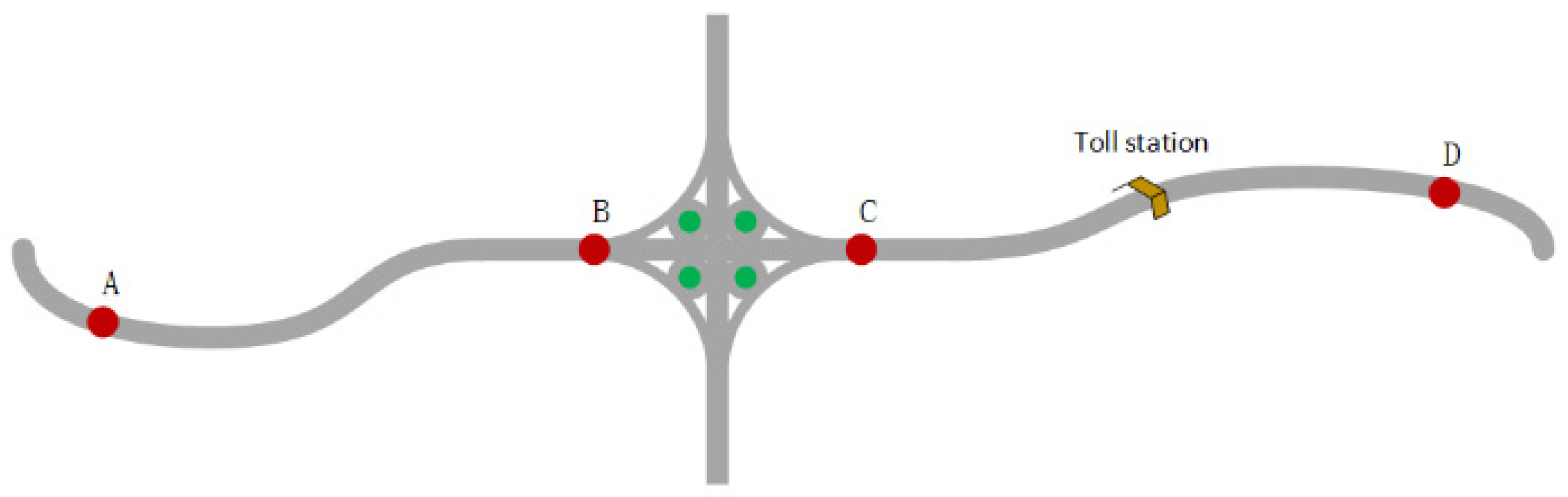
2.1.3. Toll Graph Structure

The toll graph structure involves describing the toll scheme between nodes. In many cities, the toll scheme for toll roads varies depending on the time and section of the road. Toll fees are determined by the administrative departments by setting certain toll stations on toll roads. Typically, users are required to pay the corresponding road toll each time they pass through a toll station. As these toll nodes are distributed among the detector nodes, we convert the road toll information provided by the toll stations into a connection relationship between the detector nodes. Using Orange County as an illustrative example, this issue is elaborated in detail in Figure 4 and

Table 1. Toll rates of SR261 in Orange County. It can be clearly seen that the toll varies with different sections, directions, and time. Similar changes also exist on SR241 and SR133.

Toll Point	Monday through Friday—Southbound	Account Toll Rate	Non-Account Toll Rate
Irvine Ranch	12:00 a.m.–6:59 a.m.	USD 2.69	USD 3.32
	7:00 a.m.–7:29 a.m.	USD 3.16	USD 3.32
	7:30 a.m.–8:29 a.m.	USD 3.32	USD 3.32
	8:30 a.m.–8:59 a.m.	USD 3.16	USD 3.32
	9:00 a.m.–11:59 p.m.	USD 2.69	USD 3.32
Chapman/Santiago Cyn Rd	12:00 a.m.–11:59 p.m.	No Toll	No Toll
Irvine Blvd—West NB On	12:00 a.m.–11:59 p.m.	USD 2.69	USD 2.69
Irvine Blvd—West NB Off	12:00 a.m.–11:59 p.m.	USD 2.12	USD 2.12
Irvine Blvd—West SB On	12:00 a.m.–11:59 p.m.	USD 2.12	USD 2.12
Irvine Blvd—West SB Off	12:00 a.m.–11:59 p.m.	No Toll	No Toll
Portola Pkwy—West NB On	12:00 a.m.–11:59 p.m.	USD 2.69	USD 2.69
Portola Pkwy—West NB Off	12:00 a.m.–11:59 p.m.	No Toll	No Toll
Portola Pkwy—West SB On	12:00 a.m.–11:59 p.m.	USD 2.69	USD 2.69
Portola Pkwy—West SB Off	12:00 a.m.–11:59 p.m.	USD 2.69	USD 2.69

in the scientific context. Figure 4 shows the distribution of toll stations in Orange County and Table 1 is a portion of the toll rates for roads, which were obtained from https://www.thetollroads.com (accessed on 21 January 2023).

The computation of the edge weight $A_3^{\left(i,j\right)}$ between nodes $S_i$ and $S_j$ is based on the presence of toll stations and the spatial disparity among toll stations at different locations. This is determined by the following formula:

$$A_3^{\left(i,j\right)}=\left\{\begin{array}{l}sigmoid\left(toll\left(i,j\right)\right) \mathrm{if} toll\left(i,j\right)>0\\ 0\hspace{1em}\hspace{1em}\hspace{1em}\hspace{1em}\hspace{1em}\hspace{1em} \mathrm{else}\end{array}\right.$$

(2)

where $A_3^{\left(i,j\right)}$ represents the weight between $S_i$ and $S_j$, and $toll\left(i,j\right)$ is the tolling situation between $S_i$ and $S_j$.

2.2. AASTGNet

The structure of AASTGNet is shown in Figure 5. The method consisted of two main components: a graph self-learning module for constructing the optimal graph structure, as illustrated in the left portion in Figure 5, and a spatiotemporal graph convolutional neural network model with a temporal attention mechanism for traffic flow prediction, as illustrated in the right portion in Figure 5. The first component constructs the optimal graph structure from both macroscopic and microscopic perspectives. At the macro level, the module takes three pre-defined graph structures as inputs and constructs them into the specified graph structures using Formulas (4)–(6). In each training epoch, the self-learning graph structure is built with learnable parameters according to Formula (7), adjusting the initial graph structure to generate the macroscopic graph structure for the current epoch. An initialized graph structure is constructed using the a priori relationships between the nodes, and the graph structure is fine-tuned during each round of training iterations until the macroscopically optimal graph structure is found. At the micro level, a micro-level graph structure was constructed using node information to characterize the current traffic conditions. Formulas (12) and (13) delineate the specific methodology for constructing the microscopic graph structure based on node information. Formula (14) combines the two graph structures into an optimal graph structure.

These two levels of graph structure are combined into the optimal graph structure. The second component uses a spatiotemporal graph convolutional neural network with multiple spatiotemporal convolutional layers and an attention mechanism to capture complex spatial and temporal relationships and predict traffic flow. The optimal graph structure primarily guides the computations of the GCN in this section, extracting spatial relationships among nodes. Combined with a temporal attention mechanism, it assists one-dimensional convolution operations in predicting future traffic volume. Formulas (15) and (16) illustrate the implementation process of the temporal attention mechanism, denoted as Tatt in Figure 5. Formulas (17) and (18) describe the internal operations of the GCN, while Formula (19) outlines the implementation process of spatiotemporal convolution, corresponding to the GCN + Conv module in Figure 5.

Its specific operation process can be expressed as:

$$A^{*}=g\left(\mathcal{X},\mathbb{A}\right)$$

(3)

$$\widehat{y}=h\left(\mathcal{X},A^{*}\right)$$

(4)

where $g\left(\mathcal{X},\mathbb{A}\right)$ is designed to find the optimal graph structure $A^{*}$, which can best reflect the relationship between nodes after considering the price factor, $\mathbb{A}=(A_1,A_2,A_3)$ represents a collection of graph adjacency matrices constructed based on prior knowledge, $\mathcal{X}$ denotes the node traffic data, and $h\left(\mathcal{X},A^{*}\right)$ is tailored for predicting future traffic flow $\widehat{y}$ based on node data $\mathcal{X}$ and the optimal graph adjacency matrix $A^{*}$.

2.2.1. Model the Optimal Graph Structure

This section provides a detailed exposition of the construction methodology for the optimal graph structure, categorized into macroscopic graph structure construction, microscopic graph structure construction, and the amalgamation of these two graph structures.

Macroscopic Graph Structure

The construction of the macroscopic graph structure proceeds in three steps: generating the initial graph structure, randomly generating the graph structure for the current iteration, and merging the current iteration’s graph structure with the existing graph structure.

The first step involves integrating the three pre-defined graph structures into an initial graph structure.

$$A_k\Leftarrow {\tilde{D}}_k^{-\frac{1}{2}}{\tilde{A}}_k{\tilde{D}}_k^{-\frac{1}{2}}$$

(5)

$$A^{\left(i,j\right)}=\frac{\sum _{k=1}^{N_r}{A}_k^{\left(i,j\right)}}{\sum _{k=1}^{N_r}\mathsf{\Gamma }\left[A_k^{\left(i,j\right)}\right]}$$

(6)

where ${\tilde{A}}_k=A_k+I_N$ and ${\tilde{D}}_k^{(i,i)}={\sum }_j{\tilde{A}}_k^{(i,j)}$. Equation (6) was proposed by Kipf and Welling [41] to place different graph structures in the same dimension for comparison. $\mathsf{\Gamma }$ denotes the indicator function as:

$$\mathsf{\Gamma }\left(x\right)=\left\{\begin{array}{l}1 \mathrm{if} x\ne 0\\ 0 \mathrm{else}\end{array}\right.$$

(7)

In the second step, the graph structure for the current iteration is generated. Traffic flow on the road is unidirectional, and time-varying toll schemes charge different fees for traffic flowing in different directions. In this section, a dedicated self-learning module is designed to extract the unidirectional relationships between nodes.

$$A_{\mathrm{a}\mathrm{d}\mathrm{a}}=\mathrm{R}\mathrm{e}\mathrm{L}\mathrm{U}\left(M_1{M}_2^T-M_2{M}_1^T+\mathrm{D}\mathrm{i}\mathrm{a}\mathrm{g}\left(\mathsf{\Lambda }\right)\right)$$

(8)

where $M_1,M_2\in {\mathbb{R}}^{N\times F_0}\left(F_0\ll N\right) \mathrm{and} \mathsf{\Lambda }\in {\mathbb{R}}^N$ are the learnable parameters and $\mathrm{D}\mathrm{i}\mathrm{a}\mathrm{g}\left(\mathsf{\Lambda }\right)$ diagonizes $\mathsf{\Lambda }$. $\mathrm{D}\mathrm{i}\mathrm{a}\mathrm{g}\left(\mathsf{\Lambda }\right)$ is utilized to generate the weights of diagonal positions. $\mathrm{R}\mathrm{e}\mathrm{L}\mathrm{U}$ is the activation function, which is used to enforce the sparsity of the newly generated graph structure.

In the final step, after generating the graph structure for the current iteration, the newly created structure is merged with the existing one.

$$S=\mathrm{S}\mathrm{i}\mathrm{g}\mathrm{m}\mathrm{o}\mathrm{i}\mathrm{d}\left(w_1\left(\left[A_{\mathrm{a}\mathrm{d}\mathrm{a}},A_{\mathrm{i}\mathrm{n}\mathrm{i}}\right]\right)\right)$$

(9)

$$A_{\mathrm{n}\mathrm{e}\mathrm{w}}=S\odot A_{\mathrm{a}\mathrm{d}\mathrm{a}}+\left(1-S\right)\odot A_{\mathrm{i}\mathrm{n}\mathrm{i}}$$

(10)

where $\mathrm{S}\mathrm{i}\mathrm{g}\mathrm{m}\mathrm{o}\mathrm{i}\mathrm{d}$ represents a sigmoid non-linear activation function, $A_{\mathrm{a}\mathrm{d}\mathrm{a}}$ represents the self-learning graph structure that adjusts the initial graph structure $A_{\mathrm{i}\mathrm{n}\mathrm{i}}$, $A_{\mathrm{n}\mathrm{e}\mathrm{w}}$ denotes the newly adjusted graph structure, $w_1$ represents $1\times 1$ convolutional layers, and $\odot$ indicates element-to-element multiplication. To further improve the sparsity of the model by setting a certain threshold, $A_{\mathrm{M}\mathrm{a}}$ is computed as:

$$A_{\mathrm{f}\mathrm{i}\mathrm{l}}=\mathrm{R}\mathrm{e}\mathrm{L}\mathrm{U}\left(D_{\mathrm{n}\mathrm{e}\mathrm{w}}^{-\frac{1}{2}}{A}_{\mathrm{n}\mathrm{e}\mathrm{w}}{D}_{\mathrm{n}\mathrm{e}\mathrm{w}}^{-\frac{1}{2}}-{\epsilon }_1\right)$$

(11)

$$A_{\mathrm{M}\mathrm{a}}=D_{\mathrm{f}\mathrm{i}\mathrm{l}}^{-\frac{1}{2}}{A}_{\mathrm{f}\mathrm{i}\mathrm{l}}{D}_{\mathrm{f}\mathrm{i}\mathrm{l}}^{-\frac{1}{2}}$$

(12)

where $D_2 \mathrm{and} D_3$ are diagonal matrices and $D_{\mathrm{n}\mathrm{e}\mathrm{w}}^{(i,j)}={\sum }_{j=1}^N{A}_{\mathrm{n}\mathrm{e}\mathrm{w}}^{(i,j)}$, $D_{\mathrm{f}\mathrm{i}\mathrm{l}}^{(i,j)}={\sum }_{j=1}^N{A}_{\mathrm{f}\mathrm{i}\mathrm{l}\mathrm{e}}^{(i,j)}$, and ${\epsilon }_1\in \left(\mathrm{0,1}\right)$ are the thresholds for filtering out the connections with smaller values in the matrix $A_{\mathrm{h}\mathrm{i}\mathrm{d}}$. $A_{\mathrm{f}\mathrm{i}\mathrm{l}\mathrm{e}}$ represents the filtered new graph structure, and $A_{\mathrm{M}\mathrm{a}}$ corresponds to the macroscopic graph structure.

Microscopic Graph Structure

This section delineates the methodology for constructing the micro-level graph structure, achieving this objective through convolutional operations.

$$M={\omega }_4\ast \mathrm{R}\mathrm{e}\mathrm{L}\mathrm{U}\left({\omega }_3\ast {\mathrm{R}\mathrm{e}\mathrm{L}\mathrm{U}(\omega }_2\ast \mathcal{X})\right)$$

(13)

where ${\omega }_2,{\omega }_3,{ \mathrm{and} \omega }_4$ represent convolution kernels for the convolution of the time dimension and $\mathrm{R}\mathrm{e}\mathrm{L}\mathrm{U}$ represents the ReLU non-linear activation function. $\mathcal{X}\in {\mathbb{R}}^{N\times F\times \tau }$ represents node attributes and $M\in {\mathbb{R}}^{N\times D^{\prime }}$ represents the information matrix generated from the node data, containing temporary information in the node, * represents the standard convolution operation.

The dot product is used to represent the nodes, and the matrix is processed to ensure its sparsity.

$$A_{\mathrm{M}\mathrm{i}}=\mathrm{R}\mathrm{e}\mathrm{L}\mathrm{U}\left(\mathrm{N}\mathrm{o}\mathrm{r}\mathrm{m}\left(M{M}^T\right)-{\epsilon }_2\right)$$

(14)

where ${\epsilon }_2\in \left(\mathrm{0,1}\right)$ is the threshold for filtering out the connections with smaller values in the matrix $M{M}^T$.

Optimal Graph Structure

The $\mathrm{R}\mathrm{e}\mathrm{L}\mathrm{U}$ activation function and normalization techniques are used to combine the macroscopic graph structure $A_{\mathrm{M}\mathrm{a}}$ and the microscopic graph structure $A_{\mathrm{M}\mathrm{i}}$ to obtain the optimal graph structure. The mathematical expression for this process is presented as follows:

$$A^{*}=\mathrm{N}\mathrm{o}\mathrm{r}\mathrm{m}\left(\mathrm{R}\mathrm{e}\mathrm{L}\mathrm{U}\left(A_{\mathrm{M}\mathrm{a}}+A_{\mathrm{M}\mathrm{i}}\right)\right)$$

(15)

2.2.2. Graph and Temporal Dimension Convolution

This section is primarily dedicated to exploring the spatial and temporal relationships between nodes based on the optimal graph structure. Following the work of Guo et al. [35], this module involves two key components: temporal attention and graph and temporal dimension convolution. These methods are employed to extract important temporal features and perform convolution operations on the graph structure to uncover relevant relationships between nodes in both the spatial and temporal domains.

In the temporal dimension, there are correlations between traffic conditions at different times that vary under different circumstances. To capture this variability, an attention mechanism that assigned different weights is employed to the data adaptively:

$$E=V_e·\left(\left({\left(\mathcal{X}\right)}^T{U}_1\right)U_2\left(U_3\mathcal{X}\right)+b_e\right)$$

(16)

$$E_{i,j}^{\prime }=\frac{\exp \left(E_{i,j}\right)}{{\sum }_{j=1}^{\mathsf{\tau }}\exp \left(E_{i,j}\right)}$$

(17)

where $V_e$, $b_e\in {\mathbb{R}}^{\tau \times \tau }$, $U_1\in {\mathbb{R}}^N$, $U_2\in {\mathbb{R}}^{C\times N}$, and $U_3\in {\mathbb{R}}^C$ are the weights and bias parameters that can be learned.

To extract spatial information, this paper applies spectral graph theory [42], which extends convolution operations from grid-based data to graph-structured data. In the temporal dimension, a standard convolutional neural network (CNN) is used to extract features. Node information is updated based on information from adjacent nodes. However, since spectral graph theory requires feature decomposition, it becomes computationally expensive for large-scale graphs. To address this, the Chebyshev polynomial as an approximation method is employed to alleviate the computational burden.

$$g\theta \ast \mathcal{G}\widehat{\mathcal{X}}=g\theta \left(A*\right)=\mathrm{C}\mathrm{h}\mathrm{e}\mathrm{b}\mathrm{C}\mathrm{o}\mathrm{n}\mathrm{v}\left(\widehat{A}*,\widehat{\mathcal{X}};\theta \right)=\mathrm{R}\mathrm{e}\mathrm{L}\mathrm{U}\left(\sum _{K=0}^{K-1}{\theta }_k{T}_k\left(\widehat{A}*\right)\widehat{\mathcal{X}}\right)$$

(18)

where *$\mathcal{G}$ denotes a graph convolution operation, $\mathrm{R}\mathrm{e}\mathrm{L}\mathrm{U}$ is the activation function, $\widehat{\mathcal{X}}$ represents input information, which has been processed by time attention, and $g\theta$ is a kernel filtering the signal $\widehat{\mathcal{X}}$ on the graph $\mathcal{G}$. The parameter $\theta \in {\mathbb{R}}^K$ is a vector of the polynomial coefficients. $\widehat{A}*=\frac{2}{{\lambda }_{\mathrm{m}\mathrm{a}\mathrm{x}}}{A}^{*}-I_N$, ${\lambda }_{\mathrm{m}\mathrm{a}\mathrm{x}}$ is the maximum eigenvalue of the Laplacian matrix. The recursive definition of the Chebyshev polynomial is $T_k\left(\widehat{\mathcal{X}}\right)=2\widehat{\mathcal{X}}{T}_{k-1}\left(\widehat{\mathcal{X}}\right)-T_{k-2}\left(\widehat{\mathcal{X}}\right),$ where $T_0\left(\widehat{\mathcal{X}}\right)=1,T_1\left(\widehat{\mathcal{X}}\right)=\widehat{\mathcal{X}}$.

As the graph structure in this study is defined as a directed graph, the graph structure that takes directionality into account is no longer symmetric. To address this issue, the following method is employed:

$$\widehat{\mathcal{X}}*=\mathrm{C}\mathrm{o}\mathrm{n}\mathrm{c}\mathrm{a}\mathrm{t}\left[\mathrm{C}\mathrm{h}\mathrm{e}\mathrm{b}\mathrm{C}\mathrm{o}\mathrm{n}\mathrm{v}\left(\widehat{A}*,\widehat{\mathcal{X}};{\theta }_{\mathrm{P}}\right),\mathrm{C}\mathrm{h}\mathrm{e}\mathrm{b}\mathrm{C}\mathrm{o}\mathrm{n}\mathrm{v}\left(\widehat{A}*,\widehat{\mathcal{X}};{\theta }_{\mathrm{Q}}\right)\right]$$

(19)

where ${\theta }_{\mathrm{P}}$ and ${\theta }_{\mathrm{Q}}$ are the learnable parameters, ${\widehat{A}*}^T$ is the transpose of $\widehat{A}*$, and $\mathrm{C}\mathrm{o}\mathrm{n}\mathrm{c}\mathrm{a}\mathrm{t}$ is the concatenation of different data. $\widehat{\mathcal{X}}*$ represent the input data after graph convolution processing.

After applying graph convolution operations to capture neighboring information for each node in the spatial dimension, this method utilizes one-dimensional time convolution to aggregate information related to adjacent time points. This process involves sliding a convolution kernel over the temporal axis to generate a feature map that reflects the temporal information learned by the model. The feature map is then used to update the node representations in the temporal dimension.

$${\mathcal{X}}_{\mathrm{n}\mathrm{e}\mathrm{w}}=\mathrm{R}\mathrm{e}\mathrm{L}\mathrm{U}\left(w_5\ast \left(\mathrm{R}\mathrm{e}\mathrm{L}\mathrm{U}\left(g\theta \ast \mathcal{G}\widehat{\mathcal{X}}*\right)\right)\right)\in {\mathbb{R}}^{N\times F\times \tau }$$

(20)

where $w_5$ represents the convolution kernel in the time dimension, and the activation function is $\mathrm{R}\mathrm{e}\mathrm{L}\mathrm{U}$. ${\mathcal{X}}_{\mathrm{n}\mathrm{e}\mathrm{w}}$ is not only the output of the temporal dimension convolution but also the next layer of the input data.

3. Results and Discussion

3.1. Data Set

The input data for the model consists of toll collection data and road traffic flow data from the Orange County region in the United States. The data utilized in this study were obtained from two distinct sources: the Performance Measurement System (PeMS) (available at https://pems.dot.ca.gov/, accessed on 21 January 2023) and The Toll Roads of Orange County (available at https://www.thetollroads.com, accessed on 21 January 2023). The PeMS is an extensive database of traffic information collected in real-time every 30 s by Caltrans on state highways across California, in addition to other Caltrans and partner agency data sets. The data were aggregated into 5 min intervals from raw data and encompass over 39,000 detectors installed in the major metropolitan areas of California. The Toll Roads of Orange County is a website that provides comprehensive road toll information for SR241, SR261, SR133, and SR73 in Orange County, California, USA. To perform our experiments, we employed crawlers to acquire traffic data, including the total flow and occupancy of 211 detectors in Orange County from the PeMS. Total flow denotes the total number of vehicles that passed through the corresponding detectors in a 5 min period. The detectors installed in the PeMS measure the time taken for a vehicle to pass over them, termed occupancy, which can be employed to calculate other performance measures, such as speed and delay. Moreover, as shown in Figure 6, we manually combined the road toll information as one of the node data with the total flow and occupancy. The data in this study spanned from 4 July 2022 to 4 September 2022. We partitioned the data into training, validation, and testing sets at a ratio of 6:2:2, respectively. Details of the data set are shown in

Table 2. Details of the data set.

Name	Node	Time Windows	Node Data
PEMS—Orange County	211	17,856	Flow, Occupy, Price

.

3.2. Baseline

The performance of AASTGNet was verified by conducting experiments and comparing it with other advanced models. The baselines included:

HA: Historical average, which predicts the traffic flow of the next period using the historical average of previous periods, assuming traffic flow change is a periodic process;

VAR: Vector auto-regressive model, which is a variant of ARIMA (auto-regressive integrated moving average model with a Kalman filter) that predicts subsequent data based on previous data;

FC-LSTM [43]: Long short-term memory network with fully connected LSTM hidden units;

DCRNN: Diffusion convolutional recurrent neural network, which models traffic relations on a directed graph using diffusion convolutional and recurrent neural networks (i.e., GRU and LSTM);

ASTGCN: Attention-based spatiotemporal graph convolutional network, which combines graph convolution with spatial attention to extract spatial features and standard convolution with temporal attention to extract temporal features;

AdapGL: An adaptive graph-learning algorithm for traffic prediction based on spatiotemporal neural networks. It proposes a graph self-learning module that can be applied to most graph convolutional traffic forecasting neural networks. The ASTGCN-based AdapGLA was used as its representative.

3.3. Evaluation Metrics

Suppose $\mathit{y}=y_1,\dots ,y_n$ represents the ground truth, $\widehat{\mathit{y}}={\widehat{y}}_1,\dots ,{\widehat{y}}_n$ represents the predicted values, and $\mathsf{\Omega }$ denotes the indices of observed samples; the metrics are defined as follows.

Root-Mean-Square Error (RMSE):

$$\mathrm{R}\mathrm{M}\mathrm{S}\mathrm{E}\left(y,{\widehat{y}}_i\right)=\sqrt{\frac{1}{\left|\mathsf{\Omega }\right|}\sum _{\mathrm{i}\in \mathsf{\Omega }}{\left(y_i-{\widehat{y}}_i\right)}^2}$$

(21)

Mean Absolute Error (MAE):

$$\mathrm{M}\mathrm{A}\mathrm{E}\left(y,{\widehat{y}}_i\right)=\frac{1}{\left|\mathsf{\Omega }\right|}\sum _{\mathrm{i}\in \mathsf{\Omega }}\left|y_i-{\widehat{y}}_i\right|$$

(22)

Mean Absolute Percentage Error (MAPE):

$$\mathrm{M}\mathrm{A}\mathrm{P}\mathrm{E}\left(y,{\widehat{y}}_i\right)=\frac{1}{\left|\mathsf{\Omega }\right|}\sum _{i\in \mathsf{\Omega }}\left|\frac{y_i-{\widehat{y}}_i}{y_i}\right|$$

(23)

It is worth noting that the RMSE, MAPE, and MAE serve as evaluation metrics to assess the similarity between predicted and actual values, each carrying distinct physical meanings depending on their computation methods. The MAPE characterizes the average relative error of the model’s traffic volume predictions at each node and is expressed as a percentage. The MAE represents the model’s average absolute error in predicting traffic volume at each node, measured in units such as vehicles. The RMSE effectively captures the average absolute error in traffic volume predictions at each node, assigning higher weights to larger error values. From a physical perspective, its unit is also in vehicles. In terms of physical interpretation, its unit is also in vehicles. This section provides a unified introduction to the units of evaluation metrics, and subsequent discussions will refrain from further elaboration on this aspect.

All experiments use the traffic information in the last hour to forecast the traffic flow over one hour in the future, i.e., $S=T=12$. Adam with a learning rate of 0.001 was used as the optimization method, and an early stop strategy was used to determine if the stop criteria were met. $M_1 \mathrm{and} M_2$ are set at 64, ${\epsilon }_1$ and ${\epsilon }_2$ are set as $\frac{1}{2N}$, where $N$ is the number of nodes. The size of the Chebyshev polynomial k is set to 3, the kernel of the Chebyshev polynomial and the kernel of the time convolution is set to 128, ${\theta }_P$, and ${\theta }_q$ is set to 64. The convolution kernel of $w_2$ and $w_3$ is set as $1\times 1$, The convolution kernel of $w_4$ is set as $1\times 12$, the output channels of $w_2$ and $w_3$ are set as 64, and the output channels of $w_4$ is set as 6. The number of spatiotemporal convolution blocks is set to 3. The batch size is set to 64.

In the training phase of the model, a noteworthy aspect is that the training of the macroscopic graph structure is conducted independently of the other modules. From the perspective of the paper’s design rationale, the microscopic and macroscopic graph structures form an integrated whole. However, during model training, the self-learning module for the microscopic graph and the spatiotemporal convolution module collectively constitute the backbone network of the model, while the self-learning module for the macroscopic graph operates as an independent branch. In each training iteration, the macroscopic graph structure is generated based on the initial graph structure and the self-learning module. Subsequently, the macroscopic graph structure, along with node data, is fed into the backbone network of the model for training.

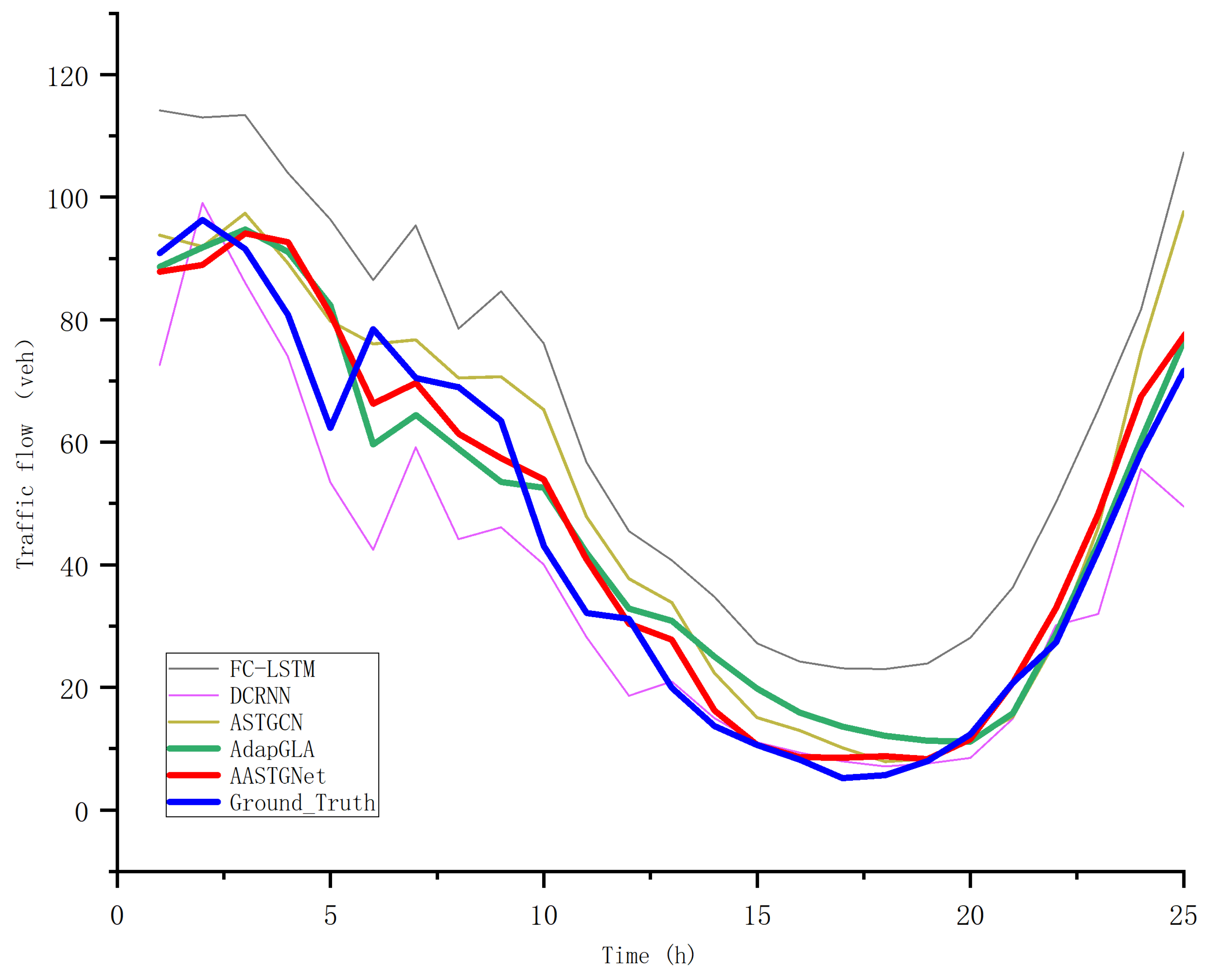
3.4. Experimental Results and Analysis

Table 3. Performance comparison of different methods for traffic flow prediction.

Model	MAE	RMSE	MAPE (%)
HA	73	167.19	44.74
VAR	24.17	61.03	15.40
FC-LSTM	12.73	25.45	0.36
DCRNN	10.54	17.62	0.26
ASTGCN	10.18	17.05	0.27
AdapGLA	8.9728	15.1618	0.2552
AASTGNet	8.6204	14.0779	0.2402

demonstrates the predictive performance of AASTGNet, as well as the remaining various baselines. The results indicated that based on evaluation metrics, such as the MAE, RMSE, and MAPE, AASTGNet exhibits higher accuracy compared to the other models. Time series methods, such as the HA and VAR, demonstrate the lowest overall performance, with the performance of the deep learning methods surpassing these approaches. Within the realm of deep learning methods, the FC-LSTM exhibits inferior performance compared to other models due to its failure to account for the spatial interactions among node sensors. In contrast to the DCRNN and ASTGCN, AdapGLA demonstrates a certain degree of improvement in predictive accuracy. This enhancement is attributed to the utilization of graph self-learning methods during the construction of the graph structure, allowing for the exploration of latent spatial relationships among nodes. AASTGNet has enhanced the existing graph self-learning methods by incorporating node information and generating the micro-level graph structure for the current moment. This improvement is particularly beneficial for addressing sudden fluctuations in road traffic flow, resulting in higher predictive performance.

Figure 7 illustrates the significant impact of a well-designed graph structure on the performance of the model across each prediction period. As the prediction interval increases, the ASTGCN and DCRNN are adversely affected by the inadequacy of the graph structure in fully capturing the inter-node relationships, leading to fluctuating prediction accuracy that even surpasses the FC-LSTM without spatial consideration. On the other hand, AdapGLA demonstrates that modeling an appropriate macro-graph structure can enhance the stability of the model in long-term prediction scenarios. Comparing the results of AdapGLA with AASTGNet, we observe that the micro-graph structure plays a crucial role in aiding the model to make more accurate predictions in each time interval. This aligns with our initial design concept of capturing the dynamic changes in the inter-node relationships through the micro-graph structure, thereby providing additional information to the model for improved prediction at every step. The specific statistical significance analysis can be found in Appendix A.

In Figure 8a, the model’s performance on toll nodes, which were nodes affected by price changes due to the presence of toll stations nearby, was analyzed. The findings revealed that AASTGNet outperformed other models in terms of accuracy on toll nodes, indicating that our proposed model effectively captures the relationship between price and traffic flow distribution on the road network. Moreover, in Figure 8b, the comparison between AASTGNet and AdapGLA is presented. It is observed that AASTGNet achieves higher accuracy than AdapGLA in each case. In particular, when the block size is set to 3, AASTGNet exhibits better performance with lower computation overhead. Notably, increasing the block size from 2 to 3 leads to a significant improvement in the model’s accuracy. On the other hand, AdapGLA’s performance remains relatively stable in normal cases, with only a small improvement in REMS observed when the block size is increased from 3 to 4. However, this comes at a considerable computational cost. To ensure a fair comparison between AdapGLA and AASTGNet, the block size was set to 3 for all experiments in this study.

To further illustrate the advantages of AASTGNet over other models for traffic flow prediction, we plot the prediction results of multiple models for the next hour at a node against the ground truth in Figure 9. As depicted in Figure 9, the optimal graph structure, benefitting from ample graph self-learning, demonstrates enhanced guidance for road traffic flow prediction. Notably, both the red curve representing AASTGNet and the green curve representing AdapGLA exhibit higher accuracy compared to other models. It is clearly illustrated that in the face of sudden fluctuations, the green curve representing AdapGLA fits the true curve relatively poorly, while the green curve representing AASTGNet has a better fit in the face of sudden arriving peaks.

4. Conclusions

In this research endeavor, we introduced and assessed AASTGNet, an advanced model tailored for predicting traffic flow by leveraging toll collection and road traffic data in Orange County, United States. The model’s architecture boasts a two-fold innovation: a graph self-learning module for optimal graph construction and a spatiotemporal graph convolutional neural network for precise traffic flow predictions. The following are three main contributions:

(1)

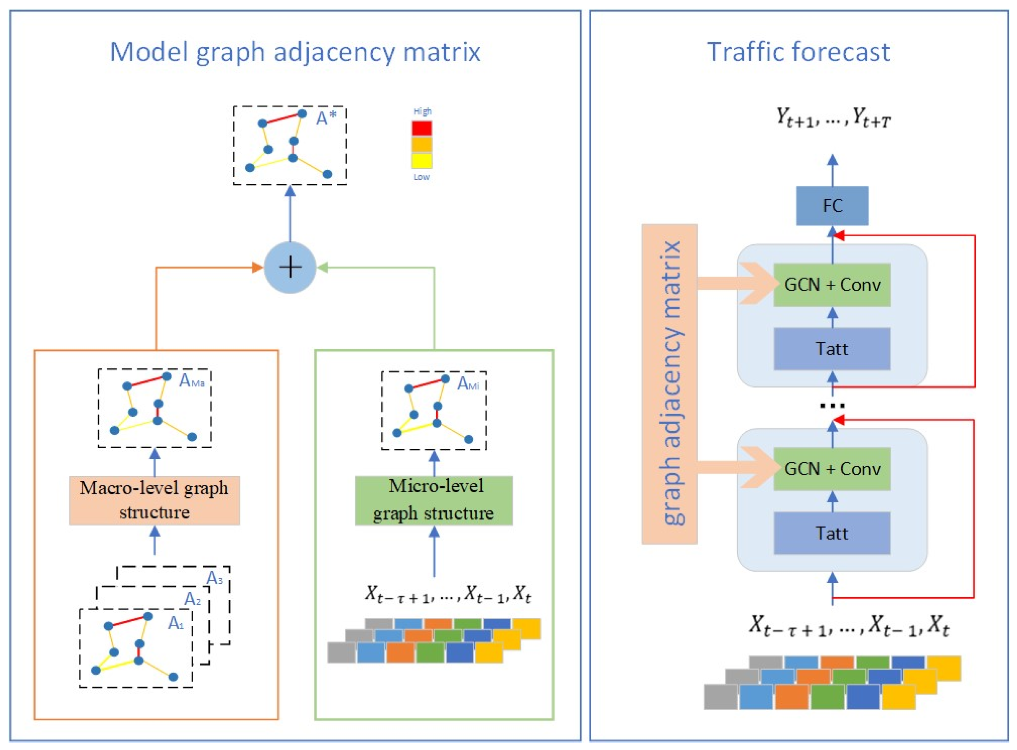
Optimal graph structure: AASTGNet pioneers a nuanced approach, amalgamating macroscopic and microscopic graph structures. The model dynamically refines the graph adjacency matrix, capturing intricate spatial relationships among traffic detectors;

(2)

Micro-level graph adjacency matrix: The introduction of a micro-level graph structure, utilizing node information for characterizing current traffic conditions, emerges as a pivotal enhancement. This addition significantly addresses sudden fluctuations in road traffic flow, enhancing predictive accuracy;

(3)

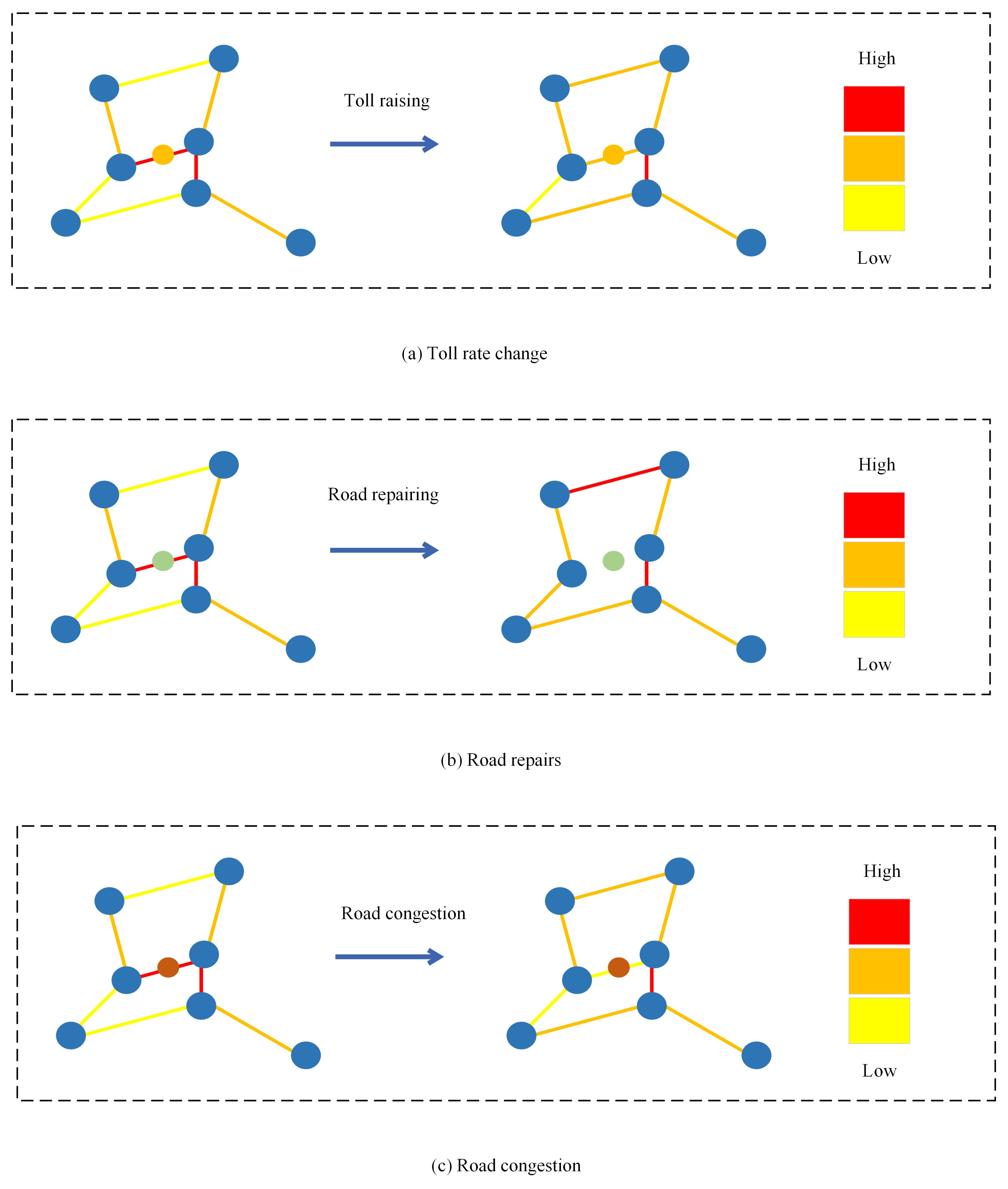
Integration of price information: AASTGNet seamlessly integrates toll data with traffic information, showcasing adaptability to scenarios influenced by toll stations. The model excels in capturing the dynamic relationship between price changes and traffic flow distribution, contributing to superior predictive accuracy.

While AASTGNet has improved in the area of traffic prediction, several avenues beckon further exploration and enhancement:

(1)

Investigating the integration of dynamic toll pricing models to enhance the adaptability of the model to evolving toll schemes, this study explores potential patterns of road toll status changes by extrapolating future adjustments in toll prices based on the current tolling situation;

(2)

Researching discerning indicators based on speed and traffic volume variations for sudden road traffic congestion, this study employs fundamental principles from traffic engineering to design control measures for managing sudden road traffic congestion. The effectiveness of the proposed measures is validated through simulation or on-site verification methods;

(3)

Investigating factors beyond changes in toll prices that influence sudden alterations in road traffic conditions, this study aims to enhance the model’s accuracy in predicting unforeseen situations;

(4)

The current model requires predicting future road traffic flow based on detection data from node sensors. Enhancements to the model can be made on the input side to accommodate a more diverse range of data.

In summary, AASTGNet emerges as a potent and versatile model for traffic flow prediction, particularly in environments influenced by toll stations. Its innovative approach to graph self-learning, coupled with the fusion of micro-level graph structures and price information, establishes AASTGNet as a frontrunner in predictive accuracy. The model holds promise for practical applications in traffic management and lays a solid foundation for further advancements in spatiotemporal traffic prediction.

References

1. Börjesson, M.; Kristoffersson, I. The Swedish congestion charges: Ten years on. Transp. Res. Part A Policy Pract. 2018, 107, 35–51. (In English) [Google Scholar] [CrossRef]
2. Li, Z.; Liang, C.; Hong, Y.; Zhang, Z. How Do On-demand Ridesharing Services Affect Traffic Congestion? The Moderating Role of Urban Compactness. Prod. Oper. Manag. 2022, 31, 239–258. (In English) [Google Scholar] [CrossRef]
3. Van Dender, K. Transport Taxes with Multiple Trip Purposes. Scand. J. Econ. 2003, 105, 295–310. (In English) [Google Scholar] [CrossRef]
4. Börjesson, M.; Eliasson, J.; Hugosson, M.B.; Brundell-Freij, K. The Stockholm congestion charges—5 years on. Effects, acceptability and lessons learnt. Transp. Policy 2012, 20, 1–12. (In English) [Google Scholar] [CrossRef]
5. Börjesson, M.; Kristoffersson, I. The Gothenburg congestion charge. Effects, design and politics. Transp. Res. Part A Policy Pract. 2015, 75, 134–146. (In English) [Google Scholar] [CrossRef]
6. Ghafelebashi, A.; Razaviyayn, M.; Dessouky, M. Congestion reduction via personalized incentives. Transp. Res. Part C Emerg. Technol. 2023, 152, 104153. (In English) [Google Scholar] [CrossRef]
7. Anas, A. The cost of congestion and the benefits of congestion pricing: A general equilibrium analysis. Transp. Res. Part B Methodol. 2020, 136, 110–137. (In English) [Google Scholar] [CrossRef]
8. Liang, Y.; Yu, B.; Zhang, X.; Lu, Y.; Yang, L. The short-term impact of congestion taxes on ridesourcing demand and traffic congestion: Evidence from Chicago. Transp. Res. Part A Policy Pract. 2023, 172, 103661. (In English) [Google Scholar] [CrossRef]
9. Arnott, R. A bathtub model of downtown traffic congestion. J. Urban Econ. 2013, 76, 110–121. (In English) [Google Scholar] [CrossRef]
10. Clements, L.M.; Kockelman, K.M.; Alexander, W. Technologies for congestion pricing. Res. Transp. Econ. 2021, 90, 100863. (In English) [Google Scholar] [CrossRef]
11. Daganzo, C.F.; Lehe, L.J. Distance-dependent congestion pricing for downtown zones. Transp. Res. Part B Methodol. 2015, 75, 89–99. (In English) [Google Scholar] [CrossRef]
12. Xiao, F.; Qian, Z.; Zhang, H.M. Managing bottleneck congestion with tradable credits. Transp. Res. Part B Methodol. 2013, 56, 1–14. (In English) [Google Scholar] [CrossRef]
13. Barrera, J.; Garcia, A. Dynamic Incentives for Congestion Control. IEEE Trans. Autom. Control 2015, 60, 299–310. (In English) [Google Scholar] [CrossRef]
14. Yu, H.; Krstic, M. Traffic congestion control for Aw–Rascle–Zhang model. Automatica 2019, 100, 38–51. (In English) [Google Scholar] [CrossRef]
15. Chiabaut, N.; Faitout, R. Traffic congestion and travel time prediction based on historical congestion maps and identification of consensual days. Transp. Res. Part C Emerg. Technol. 2021, 124, 102920. (In English) [Google Scholar] [CrossRef]
16. Pi, M.; Yeon, H.; Son, H.; Jang, Y. Visual Cause Analytics for Traffic Congestion. IEEE Trans. Vis. Comput. Graph. 2021, 27, 2186–2201. (In English) [Google Scholar] [CrossRef]
17. D’Andrea, E.; Marcelloni, F. Detection of traffic congestion and incidents from GPS trace analysis. Expert Syst. Appl. 2017, 73, 43–56. (In English) [Google Scholar] [CrossRef]
18. Ahmad, S.A.; Hajisami, A.; Krishnan, H.; Ahmed-Zaid, F.; Moradi-Pari, E. V2V System Congestion Control Validation and Performance. IEEE Trans. Veh. Technol. 2019, 68, 2102–2110. (In English) [Google Scholar] [CrossRef]
19. Li, T.; Ni, A.; Zhang, C.; Xiao, G.; Gao, L. Short-term traffic congestion prediction with Conv–BiLSTM considering spatio-temporal features. IET Intell. Transp. Syst. 2020, 14, 1978–1986. (In English) [Google Scholar] [CrossRef]
20. Qu, Z.; Liu, X.; Zheng, M. Temporal-Spatial Quantum Graph Convolutional Neural Network Based on Schrödinger Approach for Traffic Congestion Prediction. IEEE Trans. Intell. Transp. Syst. 2023, 24, 8677–8686. (In English) [Google Scholar] [CrossRef]
21. Chen, M.; Yu, X.; Liu, Y. PCNN: Deep Convolutional Networks for Short-Term Traffic Congestion Prediction. IEEE Trans. Intell. Transp. Syst. 2018, 19, 3550–3559. (In English) [Google Scholar] [CrossRef]
22. Yang, H.; Li, Z.; Qi, Y. Predicting traffic propagation flow in urban road network with multi-graph convolutional network. Complex Intell. Syst. 2023, 1–13. [Google Scholar] [CrossRef]
23. Smith, B.L.; Demetsky, M.J. Traffic flow forecasting: Comparison of modeling approaches. J. Transp. Eng. 1997, 123, 261–266. [Google Scholar] [CrossRef]
24. Williams, B.M.; Hoel, L.A. Modeling and forecasting vehicular traffic flow as a seasonal ARIMA process: Theoretical basis and empirical results. J. Transp. Eng. 2003, 129, 664–672. [Google Scholar] [CrossRef]
25. Zivot, E.; Wang, J. Vector autoregressive models for multivariate time series. Model. Financ. Time Ser. S-PLUS® 2006, 385–429. [Google Scholar] [CrossRef]
26. Zhang, S.; Li, X.; Zong, M.; Zhu, X.; Cheng, D. Learning k for kNN Classification. ACM Trans. Intell. Syst. Technol. 2017, 8, 1–19. (In English) [Google Scholar] [CrossRef]
27. Castro-Neto, M.; Jeong, Y.-S.; Jeong, M.-K.; Han, L.D. Online-SVR for short-term traffic flow prediction under typical and atypical traffic conditions. Expert Syst. Appl. 2009, 36, 6164–6173. (In English) [Google Scholar] [CrossRef]
28. Sherstinsky, A. Fundamentals of Recurrent Neural Network (RNN) and Long Short-Term Memory (LSTM) network. Phys. D Nonlinear Phenom. 2020, 404, 132306. (In English) [Google Scholar] [CrossRef]
29. Hershey, S.; Chaudhuri, S.; Ellis, D.P.; Gemmeke, J.F.; Jansen, A.; Moore, R.C.; Plakal, M.; Platt, D.; Saurous, R.A.; Seybold, B.; et al. CNN architectures for large-scale audio classification. In Proceedings of the 2017 IEEE International Conference on Acoustics, Speech and Signal Processing (ICASSP), New Orleans, LA, USA, 5–9 March 2017; pp. 131–135. [Google Scholar] [CrossRef]
30. Veyrin-Forrer, L.; Kamal, A.; Duffner, S.; Plantevit, M.; Robardet, C. On GNN explainability with activation rules. Data Min. Knowl. Discov. 2022. (In English) [Google Scholar] [CrossRef]
31. Davis, G.A.; Nihan, N.L. Nonparametric regression and short-term freeway traffic forecasting. J. Transp. Eng. 1991, 117, 178–188. [Google Scholar] [CrossRef]
32. Jeong, Y.-S.; Byon, Y.-J.; Castro-Neto, M.M.; Easa, S.M. Supervised weighting-online learning algorithm for short-term traffic flow prediction. IEEE Trans. Intell. Transp. Syst. 2013, 14, 1700–1707. [Google Scholar] [CrossRef]
33. Luo, X.; Li, D.; Yang, Y.; Zhang, S. Spatiotemporal traffic flow prediction with KNN and LSTM. J. Adv. Transp. 2019, 2019, 4145353. [Google Scholar] [CrossRef]
34. Yao, H.; Wu, F.; Ke, J.; Tang, X.; Jia, Y.; Lu, S.; Gong, P.; Ye, J.; Li, Z. Deep multi-view spatial-temporal network for taxi demand prediction. In Proceedings of the AAAI Conference on Artificial Intelligence, Orleans, LA, USA, 2–7 February 2018; Volume 32. [Google Scholar]
35. Li, Y.; Yu, R.; Shahabi, C.; Liu, Y. Diffusion convolutional recurrent neural network: Data-driven traffic forecasting. arXiv 2017, arXiv:1707.01926. [Google Scholar]
36. Guo, S.; Lin, Y.; Feng, N.; Song, C.; Wan, H. Attention based spatial-temporal graph convolutional networks for traffic flow forecasting. In Proceedings of the AAAI Conference on Artificial Intelligence, Honolulu, HI, USA, 27 January–1 February 2019; Volume 33, pp. 922–929. [Google Scholar]
37. Long, W.; Xiao, Z.; Wang, D.; Jiang, H.; Chen, J.; Li, Y.; Alazab, M. Unified spatial-temporal neighbor attention network for dynamic traffic prediction. IEEE Trans. Veh. Technol. 2022, 72, 1515–1529. [Google Scholar] [CrossRef]
38. Zhang, W.; Zhu, F.; Lv, Y.; Tan, C.; Liu, W.; Zhang, X.; Wang, F.Y. AdapGL: An adaptive graph learning algorithm for traffic prediction based on spatiotemporal neural networks. Transp. Res. Part C Emerg. Technol. 2022, 139, 103659. [Google Scholar] [CrossRef]
39. Ta, X.; Liu, Z.; Hu, X.; Yu, L.; Sun, L.; Du, B. Adaptive spatio-temporal graph neural network for traffic forecasting. Knowl.-Based Syst. 2022, 242, 108199. [Google Scholar] [CrossRef]
40. Shuman, D.I.; Narang, S.K.; Frossard; Ortega, A.; Vandergheynst, P. The emerging field of signal processing on graphs: Extending high-dimensional data analysis to networks and other irregular domains. IEEE Signal Process. Mag. 2013, 30, 83–98. [Google Scholar] [CrossRef]
41. Kipf, T.N.; Welling, M. Semi-supervised classification with graph convolutional networks. arXiv 2016, arXiv:1609.02907. [Google Scholar]
42. Bruna, J.; Zaremba, W.; Szlam, A.; LeCun, Y. Spectral networks and locally connected networks on graphs. arXiv 2013, arXiv:1312.6203. [Google Scholar]
43. Sutskever, I.; Vinyals, O.; Le, Q.V. Sequence to sequence learning with neural networks. Adv. Neural Inf. Process. Syst. 2014, 2, 3104–3112. [Google Scholar]
Figure 1. The distribution of the road sensor.
Electronics 13 00212 g001
Figure 2. Relationships between nodes changed with traffic conditions.
Electronics 13 00212 g002
Figure 3. Road geographical location and distribution of detectors in junctions. Key nodes in (a,b) are numbered, and the connection between these nodes is described in word order in the figure. (c) represents the geographical location of the road.
Electronics 13 00212 g003
Figure 4. Toll data in Orange County. The yellow nodes represent the locations of toll stations on the highway; the red route is the main toll route studied in this paper.
Electronics 13 00212 g004
Figure 5. Framework of the proposed AASTGNet. Tatt: time attention module GCN: graph convolution module; Conv: standard convolution module; FC: fully connected module.
Electronics 13 00212 g005
Figure 6. Integration of price information and traffic information at the node.
Electronics 13 00212 g006
Figure 7. The performance of different models varies with increasing prediction interval, (ac) represent the performance of each model in terms of MAE, MAPE, and RMSE at different time steps.
Electronics 13 00212 g007
Figure 8. Performance analysis of the models under different conditions: (a) a performance comparison of different deep learning models under the premise that only nodes that are greatly affected by price information are considered and (b) a performance comparison between AASTGNet and AdapGLA when different numbers of spatiotemporal convolution blocks are set.
Electronics 13 00212 g008
Figure 9. Prediction curves one hour ahead for different models at different time segments.
Electronics 13 00212 g009