Top-k Graph Similarity Search Algorithm Based on Chi-Square Statistics in Probabilistic Graphs

Abstract

Top-k graph similarity search on probabilistic graphs is widely used in various scenarios, such as symptom–disease diagnostics, community discovery, visual pattern recognition, and communication networks. The state-of-the-art method uses the chi-square statistics to speed up the process. The effectiveness of the chi-square statistics solution depends on the effectiveness of the sample observation and expectation. The existing method assumes that the labels in the data graphs are subject to uniform distribution and calculate the chi-square value based on this. In fact, however, the actual distribution of the labels does not meet the requirement of uniform distribution, resulting in a low quality of the returned results. To solve this problem, we propose a top-k similar subgraph search algorithm ChiSSA based on chi-square statistics. We propose two ways to calculate the expectation vector according to the actual distribution of labels in the graph, including the local expectation calculation method based on the vertex neighbors and the global expectation calculation method based on the label distribution of the whole graph. Furthermore, we propose two optimization strategies to improve the accuracy of query results and the efficiency of our algorithm. We conduct rich experiments on real datasets. The experimental results on real datasets show that our algorithm improves the quality and accuracy by an average of 1.66× and 1.68× in terms of time overhead, it improves by an average of 3.41×.

1. Introduction

The subgraph-matching problem [1,2] aims to find all subgraphs in a data graph that have the same structure as the query graph. The problem is widely used in compound discovery, visual pattern recognition, communication networks, community discovery, and other fields [3,4]. In practice, there is some uncertainty in the connections between objects. For example, in symptom–disease diagnosis knowledge graphs [5,6], the correlation between symptoms and diseases is uncertain and needs to be modeled using probabilistic graphs [7,8]. Specifically, vertices are used to represent symptoms (e.g., cough, fever, etc.) as well as diseases (e.g., colds, etc.), and the edges of the graph indicate the probable degree to which a given symptom is associated with a particular disease. For example, cough is a regular symptom of colds and is less likely to be associated with malaria, the probability on the edge connecting cough and cold is higher, while the probability on the edge consisting of cough and malaria is lower. In social networks, each vertex represents a person, while labels indicate a person’s field of specialization, years of experience, and other information, and the probability values on the edges indicate the strength of the connection between two people. By using subgraph-matching algorithms, we can find similar subgraphs, i.e., subgroups of people with similar labels and connectivity patterns, in these two networks. This can help us discover people with similar backgrounds and interests in different social networks, and may help recommend potential partners, friends, or career opportunities. On probabilistic graphs, since the presence or absence of an edge is correlated with its probability, the probability of its existence may be too low for many subgraphs that exactly match the structure of the query graph. Thus, when solving on probabilistic graphs using subgraph-matching algorithms on deterministic graphs, there is the problem of poor quality of matching results (too low probability) and inefficient matching.

The current method for similar subgraph search on probabilistic graphs is the ChiSeL method proposed by Shubhangi Agarwal et al. [9], which is based on the idea of the chi-square test in probabilistic statistics. By constructing observation vectors and expectation vectors for the vertices, it transforms the vertex pairs that are the most likely to be matched into the ones with the highest statistical significance. At the same time, the k most similar subgraphs to the query graph are solved efficiently by constructing an efficient index in order to quickly locate the vertex pairs with the highest similarity between the data graph and the query graph, while improving the quality of the results. The rationale of utilizing the chi-square test for subgraph matching lies in the fact that the number of labels in the actual graph is large, and the value of the component in the computed expectation vector that indicates a mismatch of vertex pairs is large, while the value of the component that indicates a match is small. When the data graph is similar to the query graph vertex pairs, the value of the component in the observation vector that indicates a match is larger and the value of the component that indicates a mismatch is smaller. Therefore, when the data graph is similar to the query graph vertex pair, the chi-square value obtained based on the expectation vector and observation vector is larger. However, at the same time, the ChiSeL algorithm still suffers from the problem of poor quality of matching results.

The main reasons for the poor quality of the results of the ChiSeL method are the following: (1) the ChiSeL algorithm calculates the expectation vector assuming that the labels in the data graph are uniformly distributed, which does not match with the distribution of the labels in the actual graph, resulting in its derived chi-square value not effectively reflecting the similarity between pairs of vertices; (2) the ChiSeL algorithm adopts the product of the probability on the edges and the chi-square value in the matching process to select extended vertices. Since the edge probabilities have already been used in the calculation of the chi-square value, multiplying them by the edge probabilities will lead to a decrease in the quality of the matching results.

To address the above problems, we propose ChiSSA (chi-square statistics-based top-k similar subgraph search algorithm), a new algorithm based on the chi-square test. Different from the ChiSeL method, which assumes that the labels are uniformly distributed in the graph, the ChiSSA method employs two new expectation vector computation strategies to enhance the effectiveness of the chi-square test based on the actual distribution of the labels in the data graph, including (1) a local computation strategy based on the distribution of labels of the vertices’ neighbors, and (2) a global computation strategy based on the distribution of labels in the whole graph. ChiSSA can find more effective chi-square values for vertex pairs based on the computed expectation and observation vectors. Further, in the query-matching phase, we first extend the results based on the size of the neighboring chi-square values. In contrast, the ChiSeL method uses the product of the edge probabilities and the chi-square values to select the extended vertices during the matching process, which can cause the problem of low quality of the matching result due to the repeated use of the edge probabilities. Secondly, in the query-matching phase, we propose a neighbor-label-based filtering method for filtering unqualified vertex pairs and reducing the number of vertex pairs that need to compute the chi-square value, thus improving the efficiency. The specific contributions of our paper are as follows:

• Propose ChiSSA, a top-k similar subgraph search algorithm based on the chi-square test on probabilistic graphs. The algorithm uses two new expectation vector computation methods based on the real distribution of labels in the data graph, including a local computation strategy based on the distribution of labels of the vertices’ neighbors, and a global computation strategy based on the distribution of labels of the whole graph, to enhance the validity of the results of the chi-square value computation.
• A new vertex expansion strategy and a neighbor-label-based filtering method are proposed for filtering ineligible vertex pairs in the query-matching phase, and reducing the number of vertex pairs that need to compute the chi-square value to improve the efficiency.
• Tests are conducted based on real datasets, and the experimental results show that the method we proposed can significantly improve the quality of the obtained results without losing the query efficiency.

The remainder of the paper is organized as follows. Section 2 discusses and analyzes related work. Section 3 describes the overall flow and specific implementation of the ChiSSA algorithm. Section 4 describes the optimization method based on neighbor label filtering. Section 5 discusses how the ChiSSA algorithm copes with multiple uncertainty situations. Finally, experimental results are shown in Section 6 and the full paper is summarized in Section 7.

2. Related Work

An undirected probabilistic graph of vertices with labels can be modeled as a quintuple $G=(V,E,\Sigma ,L,P)$, where V and E denote the set of vertices and the set of edges, respectively, $\Sigma$ is the set of labels, L is the mapping of vertices to labels, and P is the mapping of the probability of existence from edge to edge. An undirected deterministic graph of vertices with labels can be denoted as $q=(V_q,E_q,{\Sigma }_q,L_q)$, and differs from G by the absence of probabilities on edges. Explanatory notes on the notation are shown in

Table 1. Frequently used notation.

Symbol	Description
$G,q$	Data graph G, query graph q
$u,v$	Query graph vertex u, data graph vertex v
$N\left(u\right)$	Neighbor set of vertex u
$l_u$	Label of vertex u
$d_u$	Degree of vertex u
$(u,v)$	Edges formed by vertices u and v

.

Problem 1

(Top-k similar subgraph search problem on probabilistic graphs). Given a query graph $q=(V_q,E_q,{\Sigma }_q,L_q)$ and a probabilistic graph $G=(V,E,\Sigma ,L,P)$, the top-k similar subgraph search problem aims to find the top-k subgraphs in G with the highest statistical significance that are similar to q.

2.1. Subgraph-Matching Algorithms on Non-Probabilistic Graphs

Given a data graph $G=(V,E,\Sigma ,L)$ and a query graph $q=(V_q,E_q,{\Sigma }_q,L_q)$, the subgraph-matching problem aims to find all subgraphs in G that are isomorphic to q [10]. An isomorphic subgraph is a subgraph in the data graph that has exactly the same structure as the query graph. Existing algorithms for solving the subgraph-matching problem mainly include QuickSI [11], GraphQL [12], VF2 [13], and so on. The above algorithms are mainly based on the backtracking search method, which has a large time overhead to run on large-scale data graphs. There are also some algorithms for biological networks such as PathBlast [14], SAGA [15], NetAlign [16], and IsoRank [17], which mainly run on small data graphs, and also suffer from inefficiency on large-scale graphs. In order to improve the efficiency of the algorithms, the existing algorithms mainly use candidate point filtering and query vertex sorting strategies, which can effectively reduce the number of vertices that need to be traversed during the matching process, and are described below.

• Candidate point filtering. The most basic candidate point filtering method is label and degree filtering (LDF). Candidate points are generated using LDF $C\left(u\right)=$$v\in V|l_v=l_u\wedge d_v⩾d_u$. Based on this, GraphQL [12] uses local pruning and global improvement filtering methods. Among them, the local pruning method generates neighbor label strings for u according to the dictionary order and filters the candidate points by judging the containment relationship between the two strings, while the global improvement filters the candidate points by using the pseudo-subgraph isomorphism algorithm; CFL [18] proposes the following filtering rules:
  Given $X\subseteq N\left(u\right)$ and $v\in C\left(u\right)$, where $u\in V_q$, $C\left(u\right)$ is the set of candidate points, a vertex v can be removed from the candidate points of vertex u if there exists such a $u^{\prime }\in X$ that $C\left(u^{\prime }\right)\cap N\left(v\right)=\varnothing$.
  The CFL algorithm removes the candidate points that satisfy the filtering rules from the candidate point set, thus reducing the number of candidate points. Candidate point filtering can effectively reduce the number of vertices that need to be examined in the matching process, thus improving the efficiency of the algorithm.
• Query vertex sorting strategy. For the subgraph-matching problem, different matching orders greatly affect the query efficiency, so adopting a suitable sorting strategy can effectively improve the efficiency of the subgraph-matching algorithm. Even so, the time cost is still too high. Existing methods further adopt greedy strategies based on heuristic rules for speedup. For example, the RapidMatch algorithm [19] utilizes the method in [20] to find out the most tightly structured part of the query graph and prioritizes the matching from this part; the QuickSI [11] algorithm proposes a non-frequent edge prioritization method, which first constructs candidate edges for each edge in the query graph based on the labels, and then finds the edge with the smallest number of candidate edges, and selects the vertex with the smallest candidate vertices on that edge to start matching. Based on the above sorting strategy, a large number of vertices can be filtered out in the early stage of the matching algorithm, thus reducing the amount of computation.

Subgraph-matching algorithms on deterministic graphs return exact matches and cannot be used to solve similar subgraph search problems on probabilistic graphs.

2.2. Similar Subgraph Search Algorithms on Probabilistic Graphs

The extension of the underlying problems on deterministic graphs to probabilistic graphs requires the study of algorithms specialized for probabilistic graphs. Examples of such problems are frequent subgraph mining [21,22,23,24,25], clustering [26], shortest paths [27], and maximum flow [28]. The problem of subgraph search on probabilistic graphs has also been studied recently. For example, Refs. [29,30] provesthat an approximate subgraph-matching method using path decomposition is effective on fuzzy RDF graphs; meanwhile, Ref. [31] provides a detailed discussion of the state-of-the-art methods for subgraph mining on probabilistic graphs.

The latest algorithm for similar subgraph search on probabilistic graphs is the ChiSeL algorithm [9], proposed by Agarwal et al. in 2020. This algorithm is based on the chi-square test, which computes the chi-square values for the vertices with the same labels of the query graph q and the data graph G, and measures the degree of similarity between the vertices using the chi-square values, and then finds the top-k subgraphs that are similar in structure to the query graph. Specifically, the ChiSeL algorithm first forms vertex pairs with the same labels in the query graph q and the data graph G, then computes the chi-square values for all the vertex pairs, and finally prioritizes the vertex pair with the largest chi-square value as a seed to be added into the result set. At the same time, it explores its neighbors to find out the vertex pair that has the largest product of the chi-square value and edge probability as the next seed, and keeps on expanding the result set until all the query vertices are matched successfully or cannot be expanded due to a lack of matching vertex pairs. The step of calculating the chi-square value is divided into two steps, namely, calculating the expectation vector and observation vector.

• Compute the expectation vector $\mathit{E}$: The ChiSeL algorithm defaults to the idea that in the average case, the labels in the data graph are uniformly distributed, and the probability that for a vertex $\mathit{v}$, its neighbor’s label ${\mathit{l}}_{\mathit{x}}$ is $\mathbf{1}/\left|\mathit{L}\right|$, where $\left|\mathit{L}\right|$ is the total number of labels in the data graph. Based on this idea, the ChiSeL algorithm computes its expectation vector for all data graph vertices.
• Compute the observation vector $\mathit{O}$: For any vertex pair $<\mathit{u},\mathit{v}>$, the ChiSeL algorithm first generates a vertex triple (x,u,y) for vertex u, where x and y are the two neighbors of u. Correspondingly, a label triple $<{\mathit{l}}_{\mathit{x}},{\mathit{l}}_{\mathit{u}},{\mathit{l}}_{\mathit{y}}>$ can be obtained, where ${\mathit{l}}_{\mathit{x}},{\mathit{l}}_{\mathit{u}},{\mathit{l}}_{\mathit{y}}$ represent the two neighbors of u, respectively. Correspondingly, a label triad $<{\mathit{l}}_{\mathit{x}},{\mathit{l}}_{\mathit{u}},{\mathit{l}}_{\mathit{y}}>$ is obtained, where ${\mathit{l}}_{\mathit{x}},{\mathit{l}}_{\mathit{u}},{\mathit{l}}_{\mathit{y}}$ denote the labels of vertices $\mathit{x}$, $\mathit{u}$, and $\mathit{y}$, respectively. Then, the vertex pair $<\mathit{u},\mathit{v}>$ similarity is classified into three categories according to the existence of vertices with labels ${\mathit{l}}_{\mathit{x}}$ and ${\mathit{l}}_{\mathit{y}}$ in $\mathit{v}$’s neighbors, denoted as unlabeled match ${\mathit{s}}_{\mathbf{0}}$, single-labeled match ${\mathit{s}}_{\mathbf{1}}$, and double-labeled match ${\mathit{s}}_{\mathbf{2}}$, and finally, the probabilities of their occurrence in all possible worlds are enumerated for these three categories and summed up as the three components of the observation vector.

After calculating the expectation vector E and the observation vector O, the chi-square value of the vertex pair can be found according to Equation (1).

$${\chi }^2<u,v>=\sum _{i=0}^2\frac{{(O\left[s_i\right]-E\left[s_i\right])}^2}{E\left[s_i\right]}$$

(1)

Since the number of labels in the actual graph is higher, the component $s_0$ in the expectation vector that indicates a mismatch is larger. When the data graph is similar to the query graph vertex pairs, the component $s_2$ in the observation vector indicates a match is larger. Calculating the chi-square value according to Equation (1), it shows that when the data graph is more similar to the query graph vertex pair, the resulting chi-square value is larger. Conversely, when the data graph is not similar to the query graph vertex pairs, the component $s_0$ of the observation vector that indicates a mismatch is larger, while the component $s_2$ that indicates a match is smaller, and according to Equation (1), the corresponding chi-square value is smaller in this case. Based on this observation, the ChiSeL algorithm starts matching from vertex pairs with large chi-square values to obtain the top-k similar subgraph results. The ChiSeL algorithm can derive top-k similar subgraph result sets; however, as shown in example 1 below, the quality of the results it obtains is not high.

Example 1.

Given a query graph q and a data graph G in Figure 1, the purpose is to find the top-1 similar subgraph. The subgraph-matching algorithm on the graph is unable to distinguish the quality of the results sought and will return all results that match exactly. For this example, both results of Figure 1e,f would be returned, with the result shown in Figure 1f being of poorer quality. If the ChiSeL algorithm, which specializes in probabilistic graphs, is used, the algorithm first obtains the vertex pair chi-square values as shown in Figure 1c. Then, ChiSeL chooses the vertex pair $<u_1,v_1>$ with the largest chi-square value to start matching. When the matching process proceeds to the vertex pairs $<u_5,v_6>$, $<u_5,v_9>$, and $<u_5,v_{10}>$ generated by $u_5$, the edge probabilities are different from the chi-square values of $<u_5,v_{10}>$; because ChiSeL prioritizes the vertex pair with the largest product of the edge probability and chi-square value, the vertex pair $<u_5,v_9>$ is selected to be added to the result set. Since there is no vertex in the neighborhood of $v_9$ that can be matched with $u_6$, the matching process ends. The final top-1 result obtained by ChiSeL is shown in Figure 1d. Obviously, for this example, we prefer to obtain the result shown in Figure 1e.

3. ChiSSA Algorithm Based on Chi-Square Test

3.1. Basic Idea of ChiSSA Algorithm

The ChiSSA algorithm is based on the idea of the chi-square test in probabilistic statistics, which calculates chi-square values for all pairs of vertices to measure the similarity of the labeled same vertices in the data graph and the query graph, and then efficiently solves the results of the top-k similar subgraphs. Compared with the ChiSeL algorithm, our algorithm is able to find more effective chi-square values based on the actual distribution of labels in the data graph, and improve the method of selecting vertex pairs in the process of expanding the matching results, which in turn leads to higher-quality subgraph results.

Figure 2 shows the overall flow of the ChiSSA algorithm, which first generates vertex pairs based on the labels of the vertices in the query graph and the data graph (Figure 2b), followed by calculating the chi-square values based on the expectation vectors and the observation vectors of the vertex pairs (Figure 2c), and finally, searching for the top-k results based on the magnitude of the vertex pairs’ chi-square values (Figure 2d). These three steps are described separately below.

• Step 1: Generate same-label vertex pairs. Specifically, a vertex pair is composed of vertex sums with the same label. Given a query vertex u, such a vertex pair can be obtained from the label–vertex inverted table of the data graph G. For example, the complete set of vertex pairs corresponding to the query graph q of Figure 2a and the data graph G can be denoted as shown in Figure 2b.
• Step 2: Vertex pair chi-square computation. For any vertex pair $<u,v>$, first generate a vertex triad $<x,u,y>$ for vertex u, where x and y are the two neighbors of u. Correspondingly, a labeling triad $<l_x,l_u,l_y>$ is obtained, which represents the labels of vertices x, u, and y, respectively. For a vertex v in the data graph G, the vertex pair similarity is classified into the following three categories based on the presence of vertices labeled with $l_x$ and $l_y$ in its neighbors:

  -

  $s_0$: There are no vertices labeled $l_x$ and $l_y$ in the neighborhood of v;

  -

  $s_1$: Vertices labeled as $l_x$ and no vertices labeled as $l_y$ exist in the neighbors of v, or vertices labeled as $l_y$ and no vertices labeled as $l_x$ exist in the neighbors of v;

  -

  $s_2$: Both vertices labeled with $l_x$ and $l_y$ exist in the neighbors of v.

  The chi-square value is calculated as shown in Equation (1), where E is the expectation vector and O is the observation vector, which consists of the expected and observed values for the three cases $s_0$, $s_1$, and $s_2$, respectively. The expectation vector represents the distribution in the average case, while the observation vector represents the actual distribution of the two vertices of the vertex pair for the three cases $s_0$, $s_1$, and $s_2$. After calculating the expectation vector E and the observation vector O, the chi-square value of the vertex pair can be obtained by substituting into Equation (1). For example, for the same-labeled vertex pair of Figure 2b, the resulting chi-square of the vertex pair is shown in Figure 2c using the calculation in step 2.
• Step 3: Solve the top-k result set. After finding the chi-square values of all vertex pairs in step 2, the vertex pair with the largest chi-square value is first selected to be added to the result set, followed by preferentially matching the vertex pairs with the largest chi-square value among its neighbors; keep expanding until all query vertices are matched successfully or the expansion cannot continue due to a lack of vertex pairs that can be matched, and a result is obtained. The above process is repeated until k results are found. For example, for the query q of Figure 2a and the data graph G, based on the chi-square value of Figure 2c, the top-1 result obtained in step 3 is shown in Figure 2d.

The specific flow of the ChiSSA algorithm is shown in Algorithm 1. Step 1 calls the vpairGenerate function (line 3) to generate same-label vertex pairs, as shown in Figure 2b; step 2 (lines 4–7) calculates their expectation vectors and observation vectors for all the vertex pairs and computes the chi-square values according to Equation (1), and the results are shown in Figure 2c; step 3 (line 9) calls the getResult function to prioritize those vertex pairs with large chi-square values to be added to the result set, and gradually expands to obtain the top-k similar subgraph, as shown in Figure 2d. Lines 11–18 are the definition of the function vpairGenerate(q,G), which forms vertex pairs by picking vertices with the same vertex labels in V and $V_q$. The execution processes of step 2 and step 3 are described in detail below.

3.2. Vertex Pair Chi-Square Value Calculation

After generating all the vertex pairs in the first step, the chi-square value of each vertex pair needs to be computed. The chi-square value of vertex pairs is computed based on the labels present in the neighbors of the vertices to measure their similarity. Based on the neighbor labels in different cases, the vertex pairs are classified into three categories: $s_0$, $s_1$, and $s_2$. Considering Equation (1), the key to calculate the chi-square value is to find the expectation vector and observation vector of the vertex pairs, which denote the theoretical distribution and the actual observed distribution, respectively. The following describes how to solve for the expectation vector and observation vector, respectively.

In order to solve the problem that the ChiSeL algorithm does not consider the specific probability distribution of labels when calculating the expectation vector of vertex pairs, our algorithm adopts a new way of calculating the expectation vector. First, for each vertex in the data graph, according to the distribution of labels in its neighbors, we propose a local computation strategy based on the vertex degree and vertex probability degree; on this basis, considering the overall distribution of labels in the data graph, we further propose a global computation strategy based on the vertex degree and vertex probability degree, which are introduced separately below.   

Algorithm 1: ChiSSA

3.2.1. Strategies for Localized Computation of Expectation Vectors

The local computation strategy computes the expectation vector based on the distribution of labels in the neighbors of a vertex. Given any vertex pair $<u,v>$, assume that there are $N_v^{l_x}$ vertices with the label $l_x$ in the neighbor of vertex v. On average, the probability that the label $l_x$ is for any neighbor of v is $N_v^{l_x}/d_v$. Thus, the probability that there is no vertex with label of $l_x$ in the neighbors of v is $P_{LD}(\#l_x=0)={(1-N_v^{l_x}/d_v)}^{N_v^{l_x}}$. For any labeled triad $<l_x,l_u,l_y>$ generated by querying vertex u, the probability that there is no vertex with label $l_x$ or $l_y$ in the neighbors of vertex v is the degree of vertex pair $<u,v>$ matching $s_0$:

$$P\left(s_0\right)=P_{LD}(\#l_x=0)·P_{LD}(\#l_y=0)$$

(2)

The probability that vertex v has at least one neighbor with label $l_x$ is $P_{LD}(\#l_x⩾1)=1-{(1-N_v^{l_x}/d_v)}^{N_v^{l_x}}$. Thus, for the above labeled triad, the probability that the matching case of vertex pair $<u,v>$ is $s_2$ is

$$P\left(s_2\right)=P_{LD}(\#l_x⩾1)·P_{LD}(\#l_y⩾1)$$

(3)

Since the probability of occurrence of the three matching cases $s_0,s_1$, and $s_2$ sums to 1, the probability that the matching case of the vertex pair $<u,v>$ is $s_1$ is

$$P\left(s_1\right)=1-P\left(s_0\right)-P\left(s_2\right)$$

(4)

While this approach computes the expectation vector, it does not take into account the probabilistic information on the neighboring edges of the vertices. For this reason, we propose a probabilistic degree-based computation, which considers the number of occurrences of the neighbor labels of any vertex v to be related to its probabilistic degree.

Definition 1

(Label probability). Given a vertex v, if it has $n_v^{l_x}$ neighbors labeled $l_x$ that form edges with v with probabilities $p_1,p_2,p_3,\dots ,p_{n_v^{l_x}}$, the label probability degree of the vertex v is ${\delta }_v^{l_x}={\sum }_{i=1}^{n_v^{l_x}}{p}_i$ for label $l_x$.

For vertex pair $<u,v>$, if vertex v has $N_v^{l_x}$ neighbors labeled $l_x$, the probability that its label is $l_x$ for any of its neighbors is $N_v^{l_x}/d_v$, and thus the probability that there is no vertex labeled $l_x$ in the neighbors of vertex v, is $P_{LPD}(\#l_x=0)={(1-N_v^{l_x}/d_v)}^{{\delta }_v^{l_x}}$. For any label triad $<l_x,l_u,l_y>$ generated by vertex u in the query graph, the vertex pair $<u,v>$ appears to match with degree $s_0$, the label $l_x$ or $l_y$ will not appear in the neighbors of vertex v, so its probability is

$$P\left(s_0\right)=P_{LPD}(\#l_x=0)·P_{LPD}(\#l_y=0)$$

(5)

Similarly, the probability that vertex v has at least one neighbor with label $l_x$ is $P_{LPD}(\#l_x⩾1)={1-(1-N_v^{l_x}/d_v)}^{{\delta }_v^{l_x}}$. Therefore, the probability that the matching case of vertex pair $<u,v>$ is $s_2$ is

$$P\left(s_2\right)=P_{LPD}(\#l_x⩾1)·P_{LPD}(\#l_y⩾1)$$

(6)

Since the probability of occurrence of the three matching cases $s_0,s_1$, and $s_2$ sums to 1, $P\left(s_1\right)$ can be given by Equation (4).

3.2.2. Expectation Vector Global Computation Strategy

The ChiSeL algorithm solves the expectation vector with uniformly distributed labels by default, while the local computation strategy takes the individual actual data of each point as a reference, and different points with different reference data may produce inconsistent results. Unlike the above two approaches, the global computation strategy presented here considers the global actual distribution of the labels of the vertices in the data graph. Assuming that there are ${\theta }_{l_x}$ vertices labeled $l_x$ in the data graph G, on average, the probability that a label is $l_x$ is ${\theta }_{l_x}/\left|V\right|$ for any neighbor of vertex v. Considering any vertex pair $<u,v>$, if vertex v has $N_v^{l_x}$ neighbors with labels of $l_x$, then the probability that there is no vertex labeled $l_x$ among the neighbors of vertex v is $P_{GD}={(1-{\theta }_{l_x}/|V\left|\right)}^{N_v^{l_x}}$. For any label triad $<l_x,l_u,l_y>$ generated by vertex u, the vertex pair $<u,v>$ appears to match with degree $s_0$, and the labels $l_x$ or $l_y$ do not appear in the neighbors of vertex v, so its probability is

$$P\left(s_0\right)=P_{GD}(\#l_x=0)·P_{GD}(\#l_y=0)$$

(7)

The probability that vertex v has at least one neighbor with label $l_x$ is $P_{GD}(\#l_x=0)={(1-{\theta }_{l_x}/\left|V\right|)}^{{\delta }_v^{l_x}}$. Thus, for the above labeled triad, the probability that the matching case of vertex pair $<u,v>$ is $s_2$ is

$$P\left(s_2\right)=P_{GD}(\#l_x⩾1)·P_{GD}(\#l_y⩾1)$$

(8)

Similarly, $P\left(s_1\right)$ can be given by Equation (4).

For the global computation strategy, we also consider the probabilistic-degree-based case. Given a vertex pair $<u,v>$, the probability that a label is $l_x$ for any neighbor of vertex v is ${\theta }_{l_x}/\left|V\right|$. If it has $n_v^{l_x}$ neighbors labeled $l_x$, the probability that there is no vertex labeled $l_x$ in the neighbors of vertex v is $P_{GPD}={(1-{\theta }_{l_x}/|V\left|\right)}^{{\delta }_v^{l_x}}$. For any label triad $<l_x,l_u,l_y>$ generated by vertex u in the query graph, vertex pair $<u,v>$ appears to have matching degree $s_0$, the label $l_x$ or $l_y$ will not appear in the neighbors of vertex v, so its probability is

$$P\left(s_0\right)=P_{GPD}(\#l_x=0)·P_{GPD}(\#l_y=0)$$

(9)

Similarly, $P_{GPD}(\#l_x⩾1)=1-P_{GPD}(\#l_x=0)$, so the probability that the vertex pair $<u,v>$ has a matching case $s_2$ is

$$P\left(s_2\right)=P_{LPD}(\#l_x⩾1)·P_{LPD}(\#l_y⩾1)$$

(10)

$P\left(s_1\right)$ can likewise be given by Equation (4).

According to the above method, the probability values P($s_0$), P($s_1$), and $P\left(s_2\right)$ of the vertex pair $<u,v>$ about any labeled triad with matching degree of $s_0,s_1,s_2$ can be found. Assuming that vertex u involves $\eta$ labeled triples, ${\tau }_1,{\tau }_2,\cdots ,{\tau }_{\eta }$, all the expectation vectors obtained by using the above equation are $E_{{\tau }_1},E_{{\tau }_2},\cdots ,E_{{\tau }_{\eta }}$, where $E_{{\tau }_1}=[P\left(s_0\right),P\left(s_1\right),P\left(s_2\right)]$, the expectation vector of vertex pair $<u,v>$, the expectation vector of $<u,v>$ is

$$E=\sum _{i=1}^{\eta }{E}_{{\tau }_i}$$

(11)

3.2.3. Observation Vector Calculation

For any vertex pair, its observation vector can be found by enumerating all possible worlds and calculating the probability of two vertices in the vertex pair with different matching degrees. Consider any vertex pair $<u,v>$, for any labeled triple $<l_x,l_u,l_y>$ generated by querying vertex u, the matching degree of vertex pair $<u,v>$ is $s_0$ occurs if $l_x\ne l_y$, if and only if the probability of this event occurring when the number of occurrences of vertices labeled $l_x$ and $l_y$ in the neighbors of vertex v are both zero:

$$P\left(s_0\right)=P(\#l_x=0)·P(\#l_y=0)$$

(12)

where $\#l_x$ denotes the number of vertices labeled $l_x$ in the neighbors of vertex v of the data graph. Similarly, a vertex pair $<u,v>$ with a matching degree of $s_2$ occurs if and only if the vertices labeled $l_x$ and $l_y$ both occur at least once in the neighbors of the vertex v. Thus,

$$P\left(s_2\right)=P(\#l_x⩾1)·P(\#l_y⩾1)$$

(13)

Since the sum of the probabilities of occurrence of $s_0$, $s_1$, and $s_2$ is 1, the probability of occurrence of case $s_1$ can be obtained:

$$P\left(s_1\right)=1-P\left(s_0\right)-P\left(s_2\right)$$

(14)

Consider below the case $l_x=l_y$, where $s_0$ occurs as none of the vertices labeled $l_x$ appear in the neighborhood of vertex v. Thus,

$$P\left(s_0\right)=P(\#l_x=0)$$

(15)

Similarly, $s_1$ occurs as a vertex labeled $l_x$ in the neighborhood of vertex v occurs only once:

$$P\left(s_1\right)=P(\#l_x=1)$$

(16)

Similarly, since the probability of occurrence of the three cases sums to 1, the probability of occurrence of case $s_2$ is

$$P\left(s_2\right)=1-O\left(s_1\right)-O\left(s_0\right)$$

(17)

Considering Equations (12)–(17), the key to solving the observation vector is to find the probabilities that the number of occurrences of any of the labels in the neighbors of vertex v is 0, 1, and greater than or equal to 1, as detailed below.

Assuming that vertex v has $\psi$ neighbors labeled $l_x$, and the probabilities of the edges they form with v are $p_1^{l_x},p_2^{l_x},\cdots ,p_{\psi }^{l_x}$, then $P(\#l_x=0)$ is equal to the probability that none of the edges formed by v and the above vertices exists, which can be given by the following equation:

$$P(\#l_x=0)={\Pi }_{i=1}^{\psi }(1-p_i^{l_x})$$

(18)

The probability that the number of occurrences of a vertex labeled $l_x$ in the neighborhood of vertex v is greater than or equal to 1 can be quickly derived from Equation (17):

$$P(\#l_x⩾1)=1-P(\#l_x=0)$$

(19)

Similarly, the probability that the label $l_x$ occurs only once in the neighbors of vertex v is

$$P(\#l_x=1)=\sum _{i=1}^{\psi }[p_i^{l_x}·\sum _{j\ne i}(1-p_j^{l_x})]$$

(20)

According to the above formula, the probability that a vertex pair $<u,v>$ matches about any labeled triad with the degree of $s_0,s_1,s_2$ cases can be found. Assuming that vertex u involves a total of $\eta$ labeled triples as ${\tau }_1,{\tau }_2,\cdots ,{\tau }_{\eta }$, all the observation vectors obtained by using the above formula are $O_{(}{\tau }_1),O_{(}{\tau }_2),\cdots ,O_{(}{\tau }_{\eta })$, where $O_{(}{\tau }_1)=[P\left(s_0\right),P\left(s_1\right),P\left(s_2\right)]$, the observation vectors of the vertex pair $<u,v>$, the observation vector is

$$O=\sum _{i=1}^{\eta }{O}_{{\tau }_i}$$

(21)

3.2.4. Index Construction

Based on the above discussion, its chi-square value can be obtained for all vertex pairs. To speed up this computational process, we construct corresponding indexes based on the data graph for storing vertex and probability information. Specifically, the indexes are constructed as follows:

• Label–vertex inverted index: The label–vertex inverted index stores the mapping between labels and vertices in the data graph. The index constructed from the data graph G in Figure 1 is shown in

  Table 2. Label–vertex inverted table.

  Label	Vertex	Label	Vertex
  A	$v_1,v_4$	E	$v_6,v_9,v_{10}$
  B	$v_2$	F	$v_7,v_{11}$
  C	$v_3$	G	$v_8$
  D	$v_5$

  . The label–vertex inverted index is mainly used for the generation of vertex pairs. Based on the labels of the vertices in the query graph, accessing the label–vertex inverted index can quickly obtain the set of vertices in the data graph that have the same labels as them.
• Neighbor label index: For each vertex in G, the neighbor label index stores the number of times each label appears in its neighbors, while the sum of the probabilities of these neighbors forming an edge with that vertex is pre-computed.

  Table 3. Neighbor label index.

  Vertex	Neighborhood Label	Number of Occurrences	Label Probability
  $v_1$	A	1	0.8
  	B	1	0.9
  	C	1	0.9
  	D	1	0.9
  $v_2$	A	2	1.4
  	C	1	0.7
  $v_3$	A	2	1.2
  	B	1	0.7
  $v_4$	A	1	0.8
  	B	1	0.5
  	C	1	0.3
  	D	1	0.9
  $v_5$	A	2	1.8
  	E	3	1.3

  shows the structure of the neighbor label index constructed based on some of the vertices in the data graph G of Figure 1. During the computation of the expectation vector, based on a given vertex with a label, the neighbor label index can be used to quickly obtain the probability degree of a specific label in a vertex’s neighbors, as well as the number of times that label appears.
• Neighbor label probability index: In order to accelerate the solving of observation vectors, for each vertex in the data graph, we pre-calculated the probability of each kind of label appearing 0 times, 1 time, and greater than or equal to 1 time in their neighborhoods according to Equations (18)–(20).

Example 2.

In the data graph G of Figure 1, the probability that the E label appears 0 times in the neighbors of vertex $v_5$ can be derived from Equation (18): $p(\#E=0)=(1-0.1)\times (1-0.8)\times (1-0.4)=0.108$.

3.3. Top-k Result Matches

The process of solving the top-k result set is based on selecting and expanding the vertex pairs based on their chi-square values. The vertex pair with the largest chi-square value is first selected and preferentially matched with the vertex pair with the largest chi-square value among its neighbors. This process expands until all query vertices are matched successfully or no further expansion is possible to obtain a result. The process is then repeated until k results are found. The ChiSSA algorithm inserts all vertex pairs according to their chi-square values into a big-topped heap called the initial heap; subsequently, the vertex pairs at the top of the heap are sequentially selected as the initial vertex pairs of the expansion result.

For each vertex pair selected from the initial heap, its neighbor vertex pairs need to be searched until the end of the matching process. Assuming that the selected vertex pair is $<u,v>$, a vertex pair $<n_u,n_v>$ consisting of vertices with the same labels in the neighbors of vertices u and v will be selected and inserted into another big-topped heap, called the secondary heap, with the top of the vertex pair of the heap’s ${\chi }_{<n_u,n_v>}^2$ value being maximized. After selecting a heap’s top vertex pair, the vertex pair is used as a new seed vertex pair to continue searching its neighbor vertex pairs. The neighbor search is repeated until the query graph completes the matching or the subgraph in the target graph cannot continue to expand due to the lack of eligible vertex pairs. The above steps are repeated k times to find the top-k result set.

Algorithm 2 is the pseudocode of the getResult function, which first adds the vertex pair with the largest chi-square value to the result set and marks it as visited (lines 3–6); and then extends the similar subgraph results from that vertex pair using the breadth-first search method (lines 7–24), where $VP\left[w_2\right]$ in line 16 serves to gather all the same-labeled vertex pairs associated with query point $w_2$ according to the “query point–vertex pair” inverted table. Here, the “query point–vertex pair” inverted table is used to organize the set of vertex pairs according to the query points so as to quickly find all the vertex pairs associated with a particular query point. Based on the input query graph, the inverted table is generated by scanning the set of vertex pairs with the same label once. The judgment condition in line 17 requires two vertex pairs to be connected, i.e., $(v_1,v_2)$ is the edge in the data graph and $(w_1,w_2)$ is the edge in the query graph; finally, the above process is repeated k times to find the top-k similar subgraph result.

Algorithm 2: getResult

3.4. Algorithm Analysis

Given the data graph $G=(V,E,L,\Sigma ,P)$, query graph $q=(V_q,E_q,L_q,{\Sigma }_q)$, and the number of query results k, the time complexity and spatial complexity of the query phase of the ChiSSA algorithm with index construction are analyzed as follows.

3.4.1. Query Stage

The time overhead of the query phase has three steps.

• Generate same-label vertex pairs. This operation can be generated directly from the “label–vertex” inverted table. In this process, the “query point–vertex pair” inverted table is generated at the same time. Suppose the set of vertex pairs is $VP$. Since $\left|VP\right||V_q| \times |V|$ is small and can be regarded as constant, the time cost of this operation can be expressed as $O\left(\right|V\left|\right)$.
• Calculate the chi-square value. The observation vectors in this step are computed in the same way as ChiSeL, and its time cost is $O\left(\right|E\left|\right)$, similarly, the expectation vectors in ChiSSA are computed with the same time complexity as the observation vectors, and then its time cost is also $O\left(\right|E\left|\right)$, so this is the time cost of step (2).
• Solving the top-k result set. First, analyze the time complexity of solving each result in the top-k result set. The time complexity of inserting vertex pairs into the initial heap is $O\left(\right|V|\ast log|V\left|\right)$, and the time complexity of constructing the subheap by selecting the top vertex pair of the heap each time is $O(d_v\ast log{d}_v)$, where $d_v$ is the average degree of the graph G. Consider $\left|E\right|⩽{\left|V\right|}^2$, then $d_v=2\ast \left|E\right|/\left|V\right|\sim O\left(\right|V\left|\right)$. Therefore, the time complexity of constructing the subheap each time is $O\left(\right|V|\ast log|V\left|\right)$, and this step is executed at most $|V_q|$ times, then the time complexity of solving a single result is $O\left(\right|V_q|\ast |V|\ast log|V\left|\right)\sim O\left(\right|V|\ast log|V\left|\right)$. Therefore, the overall time complexity of the ChiSSA algorithm is $O\left(\right|E|+k\ast |V|\ast log|V\left|\right)$.

The space overhead is mainly used for the initial heap and subheap. The size of the initial heap is the number of vertex pairs $O\left(\right|V\left|\right)$ and the size of each subheap is $O\left(d_v\right)\sim O\left(\right|V\left|\right)$, so the overall space complexity of the algorithm is $O\left(\right|V\left|\right)$.

3.4.2. Index Construction

The time complexity of constructing the three indexes is analyzed as follows. (1) “Label–vertex” inverted index: constructing the label–vertex inverted index requires one traversal of the vertices in the data graph, and its time complexity is $O\left(\right|V\left|\right)$. (2) Neighbor label index: constructing a neighbor label index requires one traversal of the neighbors of all vertices, which is equivalent to one traversal of the edges of the whole graph, and its time complexity is $O\left(\right|E\left|\right)$. (3) Neighbor label probability index: the same as (2), it requires one traversal of the neighbors of all vertices, so its time complexity is. In summary, the overall time complexity of index construction is $O\left(\right|V|+|E\left|\right)$.

The label–vertex inverted index stores every vertex in the data graph, so its space complexity is $O\left(\right|V\left|\right)$; the neighbor label index stores the number of occurrences with probability for labels that have appeared in each vertex’s neighbors, so the worst-case space consumption is $\left|V\right|\ast |\Sigma |$. Even if the number of labels in the graph is high, the actual number of labels that have appeared in each vertex neighbor is at most the number of its neighbors, so the space complexity of the neighbor label index is $O\left(\right|V|\ast d_v)\sim O\left|E\right|$; the neighbor label probability index needs to record the probability of all labels appearing various times in each vertex neighbor. Therefore, the space complexity of the neighbor label probability index is $O\left(\right|V|\ast |\Sigma \left|\right)$.

4. Algorithm Optimization

Although the ChiSSA algorithm can find the top-k similar subgraph results with high accuracy, it needs to calculate the chi-square of all vertex pairs, which is a large amount of computation. To address this problem, we propose an optimization method based on neighbor label filtering to generate vertex pairs, which can reduce the size of the set of generated vertex pairs, and thus, improve the algorithm’s efficiency.

Definition 2

(Accuracy of results [9]). Given a query graph $q=(V_q,E_q,L_q,{\Sigma }_q)$ and a top-k result set $res=r_1,r_2,\cdots ,r_k$, where $r_i=(V_{r_i},E_{r_i})$. Result accuracy, $acc={\sum }_{i=1}^k|E_{r_i}|/(k\ast |E_q\left|\right)$.

Lemma 1

(Filter criteria). Given a vertex pair $<u,v>$, where $u\in V_q,v\in V,\forall p\in N\left(u\right)$, if there exists no satisfaction $q\in N\left(v\right)$, the addition of the result set does not improve the accuracy of the result.

Proof. 

Proof by contradiction. Assuming that the addition of vertex pairs $<u,v>$ to the result set improves the accuracy of the results, there must exist $p\in N\left(u\right),q\in N\left(v\right)$ such that $(p,u),(q,v)\in E$, and $l_u=l_v\wedge l_p=l_q$, which contradicts the conditions of Lemma 1. Proof completion.    □

According to the filtering criterion, for a vertex pair $<u,v>$, if the labels of all neighbors of u are not the same as the neighbor labels of v, it can be filtered out.

Algorithm 3 shows the pseudocode of the vertex pair generation method vpairGenerate+ based on the neighbor label filtering optimization. For all the vertex pairs generated by the vpairGenerate method, counting is used to determine whether they meet the filtering criteria. The following is an example of vertex pairs. First, the array A is initialized as well as the counter $count$ (lines 3–4), and for all neighbors of u, the corresponding label position in the array A is marked as 1 (lines 5–7). If any of v’s neighbors has the same label as u’s neighbor’s label, 1 counter is added to $count$ (lines 8–11). If the final counter $count$ value is 0, it means that all the labels in the neighbors of u and v are not the same, and according to the filtering criterion, the vertex pair is removed from the set of vertex pairs (lines 12–13). Finally, the filtered set of vertex pairs ${VP}^{\prime }$ is returned.

Algorithm 3: vpairGenerate+

5. Analysis of Other Situations

Previously, we discussed the case where the ChiSSA algorithm solves for similar subgraph outcomes on probabilistic graphs with labeled vertices, and the uncertainty in such probabilistic graphs exists only on the edges. In this section, we briefly describe how to deal with other types of uncertainty cases.

5.1. Edge Label

For the case that the edges in the data graph are also labeled, the labels of both vertices and edges in the query result need to be the same as those in the query graph. In order to meet the above requirements, when constructing the labeled triples, the vertex labels are combined with the labels of the corresponding edges, and when calculating the degree of matching of the triples, only when the vertex labels and the edge labels are the same is it recorded as a successful match.

5.2. Uncertain Vertex

Consider the case where the vertices in the data graph also have uncertainty, each vertex is associated with a probability value which indicates the probability of the existence of that vertex. For this case, multiply the edge probability with the vertex probability as the new edge probability, based on which the corresponding result can be obtained using our method. For example, assuming that the existence probabilities of vertices u, v, and w are $p_u$, $p_v$, and $p_w$, respectively, and the existence probabilities of edges $e_1=(u,v)$ and $e_2=(w,v)$ are $p_1$ and $p_2$, respectively, the probabilities of edges $e_1$ and $e_2$ are updated to $p_1^{\prime }=p_1{p}_u{p}_v$, $p_2^{\prime }=p_2{p}_w{p}_v$, respectively, based on our method, and then the results can be obtained.

6. Experimentation and Analysis

6.1. Experimental Setup

Experimental environment: The hardware configuration used for the experiments is with 1 TB of running memory; the operating system is Ubuntu 20.04.6 LTS, and all the algorithms are implemented in C++.

Comparison algorithms: The main comparison algorithms for the experiment are the ChiSeL [9], ChiSSA-LD, ChiSSA-LPD, ChiSSA-GD, and ChiSSA-GPD algorithms. Where ChiSSA-LD and ChiSSA-LPD denote local algorithms based on vertex degree and vertex probability degree, respectively, and ChiSSA-GD and ChiSSA-GPD denote global algorithms based on vertex degree and vertex probability degree, respectively. Our experiments do not include subgraph search algorithms on deterministic graphs because the experimental results in Ref. [9] have verified the inefficiency of these algorithms on deterministic graphs.

Datasets: We employ nine real datasets in our experiments, as shown in

Table 4. Datasets.

Dataset	$\left|\mathit{V}\right|$	$\left|\mathit{E}\right|$	Avg. Degree	Labels
soc-flickr	513,970	3,190,452	12.4	70
yeast	3112	12,519	8.0	3112
dblp	226,414	716,460	6.3	15
youtube	1,134,890	2,987,624	5.3	25
soc-FourSquare	639,015	3,214,986	10.1	27
soc-catster	149,701	5,449,275	72.8	30
PPI	140,098	23,084,050	329.5	80
IMDB	1,199,921	3,782,464	6.3	60
yago	876,252	13,668,320	31.2	70

. Among these datasets, soc-flickr, soc-FourSquare, soc-catster, yeast, dblp, and youtube can be downloaded on networkrepository (networkrepository.com, accessed on 5 September 2023). PPI is the COG mapping of proteins and their links, which can be retrieved from the STRING DB (string-db.org, accessed on 5 September 2023). Yago (yago-knowledge.org, accessed on 5 September 2023) is an open-source knowledge graph consisting of extracted entities and relations from Wikipedia, WordNet, and GeoNames. IMDB (konect.cc, accessed on 5 September 2023) is a dataset with information on movies, actors, directors, etc.

Evaluation metrics: The evaluation metrics used in the experiment are result quality and runtime, respectively, where result quality can be further categorized into result accuracy and result probability. The formal definition of result accuracy is shown in Definition 2, which reflects the degree of similarity between the obtained results and the structure of the query graph, independent of the size of the probabilities on the edges in the results. The result probability sum is defined as shown in Definition 3. This metric represents the sum of the probability values on the edges in the result subgraph, and the larger the result quality value, the higher the probability that the result obtained exists. The combination of the two can reflect the quality of the result from the perspective of structural similarity and the probability of existence.

Definition 3

(Sum of result probabilities). Given a top-k result set $res=\{r_1,r_2,\cdots ,r_k\}$ of a query graph q, where $r_i=(V_{r_i},E_{r_i})$, assuming that the set of edges $E_{r_i}$ consists of $e_{r_i}^1,e_{r_i}^2,e_{r_i}^3,\cdots ,e_{r_i}^{|E_{r_i}|}$, the result probability sum $quality={\sum }_{i=i}^k{\sum }_{j=1}^{|E_{r_i}|}p\left(e_{r_i}^j\right)$.

6.2. Experimental Results and Analysis

Setting parameter k = 5, 30 query graphs each with vertices 4, 6, 8, 10, 12, 14, and 16 are randomly generated from the data graphs for the query operation, and the accuracy, result probability sum, and running time of the ChiSeL, ChiSSA-LD, ChiSSA-LPD, ChiSSA-GD, and ChiSSA-GPD algorithms to find the top-k result set are recorded.

6.2.1. Comparison of Result Accuracy

Figure 3 shows a comparison of the accuracy of the results obtained by the three algorithms for different sizes of query graphs on nine datasets. The following observations are made based on Figure 3:

• The accuracy of the results obtained by the four ChiSSA algorithms is much higher than that of the ChiSeL algorithm on almost all the datasets, where the accuracy of the results obtained by the global computation strategy is higher than that of the local computation strategy.
• As the query graph size increases, the accuracy of the results obtained by the five algorithms decreases, but the accuracy of the results obtained by the four ChiSSA algorithms proposed is still much higher than that of the ChiSeL algorithm. On most of the datasets, the accuracy of the results obtained by the ChiSSA algorithms can be maintained at a high level. There are two main reasons for this: first, the ChiSeL algorithm assumes that all labels have exactly the same probability of occurrence when solving for the expected value, which is not realistic. In contrast, the ChiSSA algorithm considers the specific distribution of labels when calculating the expectation value, which makes the chi-square value obtained by the ChiSSA algorithm more reflective of the similarity of vertex pairs.
• The accuracy of the results obtained by the ChiSSA algorithm based on the global computation strategy is higher than that obtained by the local computation strategy because the local computation strategy only takes into account the distribution of labels in the neighbors of individual vertices, while the global computation strategy considers the overall probability distribution of labels in the data graph.

It should be noted that for the yeast, the accuracy of the results obtained by the five methods is the same, at 0.2, which is because the number of labels and the number of vertices in these datasets are closer to or the same as the number of vertices, so that there is only a unique subgraph in the data graph that has the exact same structure as the query graph, and therefore, the accuracy of the results obtained according to Definition 2 is 0.2.

6.2.2. Comparison of Sum of Result Probabilities

Figure 4 illustrates the comparison of the sum of the result probabilities found by the ChiSSA algorithm and the ChiSeL algorithm on the nine datasets. The following observations are made based on Figure 4: (1) The resultant probability sums obtained by the four ChiSSA algorithms are much better than the ChiSeL algorithm on almost all the datasets, which is because the chi-square values computed by the ChiSSA algorithms better reflect the similarity of the vertex pairs, and thus the resultant probability sums are better. (2) On the yeast datasets, the resultant probability sums are also identical because the number of labels is close to the number of vertices, which makes the five algorithms produce consistent results.

6.2.3. Comparison of Calculation Time of Chi-Square Values

Figure 5 shows the time consumption of the ChiSeL algorithm, ChiSSA algorithm, and ChiSSA+ algorithm to compute the chi-square value for different sizes of query graphs on nine datasets, where ChiSSA+ denotes the ChiSSA algorithm optimized with neighborhood vertex filtering. According to Figure 5, there are the following observations:

• The running time of the base ChiSSA algorithm is about 30% higher than that of the ChiSeL algorithm because the ChiSeL algorithm computes the expectation vectors with default labels that are uniformly distributed so that the expectation vectors can be obtained before the query arrives; comparatively, the ChiSSA algorithm needs to spend more time to compute the expectation vectors.
• The ChiSSA+ algorithm takes less time to run than the ChiSeL algorithm after optimization with neighbor label filtering, because the use of neighbor labels filters out more pairs of vertices, which effectively reduces the computations of the algorithm.
• As the size of the query graph increases, the overall computation time is increased. The reason is that the number of vertex pairs to be computed increases with the number of query graphs.

  Table 5. Comparisons of computing number of vertex pairs.

  Query Graph Size	Vertex Pair Number
  	ChiSSA	ChiSSA+
  4	56,292	17,761
  6	84,510	28,696
  8	113,319	41,275
  10	141,373	51,620
  12	169,272	56,456
  14	189,799	64,566

  counts the comparison of the number of vertex pairs that need to be computed before and after using the neighbor label filtering optimization on the dblp dataset, which is used to explain the effectiveness of the neighbor label filtering optimization.

Figure 6 shows the overall running time of the ChiSeL algorithm, ChiSSA algorithm, and ChiSSA+ algorithm on the nine datasets with the parameter k set to 5 and the number of vertices of the query graph set to eight. It shows that the ChiSSA+ algorithm with filtering optimization has the highest running efficiency.

6.2.4. Effect of Parameter k on Experimental Results

The parameter k is set to 5, 10, 15, 20, 25, and 30 for the nine datasets in Table 4, and the query operation is carried out using 30 query graphs, in which the number of vertices of all the query graphs is eight. The statistical results are shown in Figure 7, Figure 8 and Figure 9.

Figure 7 demonstrates the results’ accuracy. As can be seen from Figure 7, with the change in the k value, the overall accuracy of the results obtained by the ChiSSA algorithm is much higher than that of the ChiSeL algorithm on almost all the datasets; the accuracy of the results obtained by the ChiSeL algorithm decreases significantly as k increases, while the two ChiSSA algorithms are still able to maintain a higher accuracy of the results, which is because the expectation vectors calculated by the ChiSeL algorithm do not reflect the real situation well, which leads to the low accuracy of the obtained top-k results.

Figure 8 demonstrates the results’ probability sums. As can be seen from Figure 8, on almost all datasets, the probability sum of the results obtained by all ChiSSA algorithms is much higher than that of the ChiSeL algorithm as a whole, which is because the chi-square values obtained by ChiSSA algorithm are more effective, which in turn means they obtain results with a higher probability of existence; as the value of k increases, the probability sum of the results obtained by the ChiSSA algorithm is always higher than that of the ChiSeL algorithm.

Figure 9 shows the overall running time. From Figure 9, it can be seen that the overall running time grows linearly as the value of k increases, which is because the third step of the algorithm, solving for the top-k results, occupies the main running time, and the larger the value of k, the longer the time used.

In particular, on yeast, the ChiSSA and ChiSeL algorithms can only obtain one result for any query, since their label counts are close to the vertex counts, so their result accuracies $acc=1/k$. Similarly, the result probability sums remain constant as the k value increases.

Comprehensively comparing the above results, it can be concluded that when solving the top-k similar subgraphs on probabilistic graphs, the ChiSSA algorithm can be more efficient than the ChiSeL algorithm in providing top-k results with better quality.

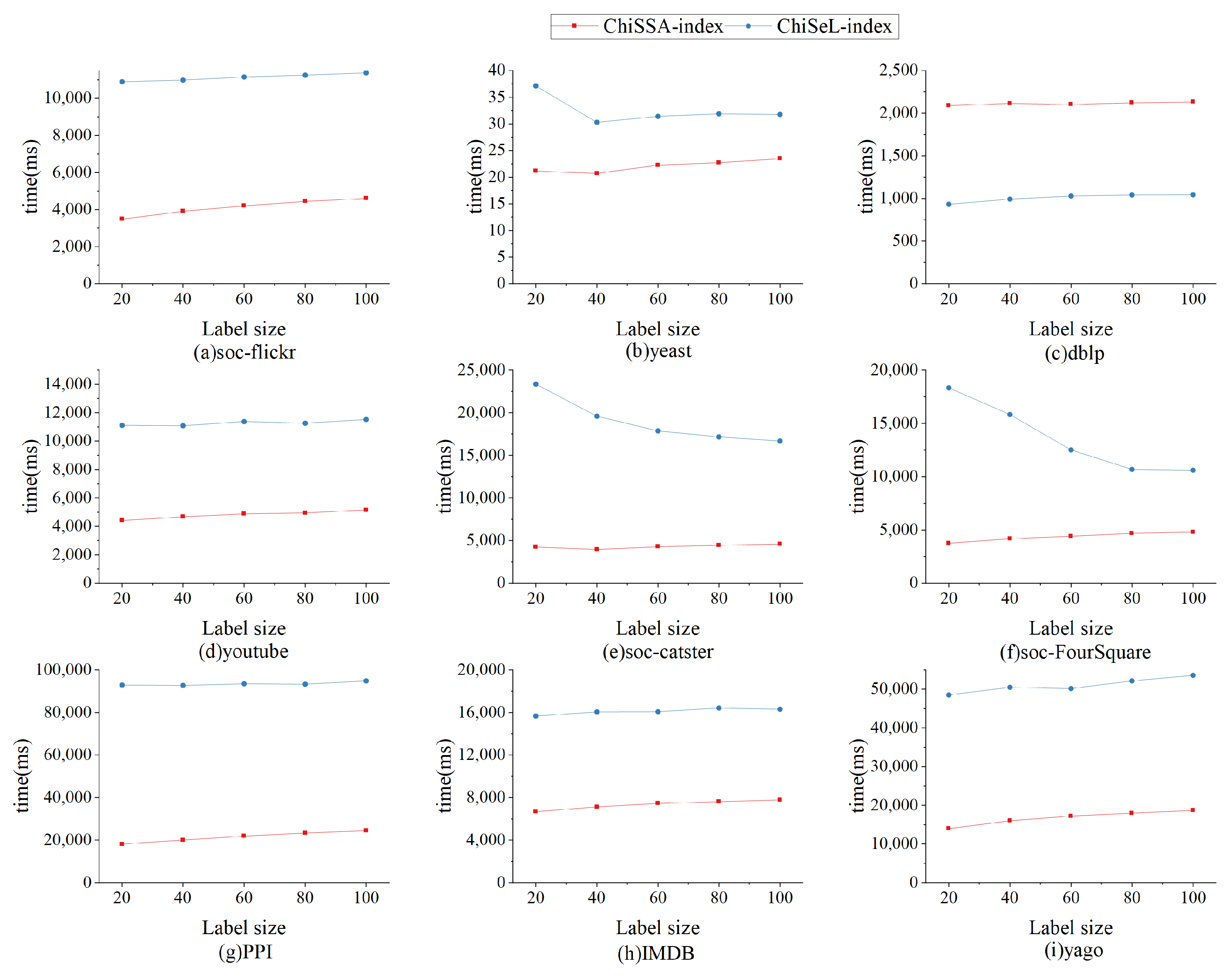
6.2.5. Index Experiment

The nine datasets in Table 4 are randomly assigned the number of labels 20, 40, 60, 80, and 100 to study the effect of the number of labels on the index size as well as the index running time, and the results are shown in Figure 10 and Figure 11.

Figure 10 shows the effect of the number of labels on the index size. From Figure 10, it can be seen that ChiSSA-index outperforms ChiSeL-index on all datasets; as the number of labels increases, the index size increases, the number of neighboring label types maintained by each vertex increases also increases, and the size of the neighboring label index and neighboring label probability index increases, with a limited effect on the “label–vertex” inverted index.

Figure 11 shows the effect of the number of labels on the index construction time. As shown from Figure 11, the ChiSSA-index exhibits higher efficiency relative to the ChiSeL-index. We observe that the ChiSSA-index is able to complete the index construction process faster under the same dataset and hardware environment.

7. Conclusions

Aiming at addressing the low quality of the results obtained by the existing algorithms for solving top-k similar subgraphs on probabilistic graphs, we propose an algorithm based on the chi-square test, ChiSSA. According to the actual distribution of labels in the data graph, the algorithm employs two new strategies for calculating the expectation vectors, namely, the local expectation vector computation based on the distribution of the vertices’ neighbors and the global expectation vector computation based on the distribution of labels of the whole graph. The local computation strategy computes the expectation vector based on the distribution of labels in the vertex neighbors, and the global computation strategy computes the expectation vector based on the distribution of labels in the data graph. Further, we propose an optimization strategy to simultaneously improve the results’ quality and reduce the number of vertex pairs to be computed. Finally, we conduct experiments on real datasets, and the experimental results show that (1) in terms of result quality, the ChiSSA algorithm is better than the ChiSeL algorithm regarding both result accuracy and result probability sum. In terms of result accuracy, the ChiSSA algorithm is about 20% higher than the ChiSeL algorithm overall, and in the best case the accuracy is nearly double; in terms of result probability sums, the results obtained by the ChiSSA algorithm are about double that of the ChiSeL algorithm. (2) In terms of runtime, the ChiSSA algorithm has a lower chi-square-value computing time than the ChiSeL algorithm, and in the best case is about an order of magnitude faster than existing methods.