

Using Medical Data and Clustering Techniques for a Smart Healthcare System

 , ,
, , 
Abstract
:1. Introduction
2. Clustering Techniques and Applications for Medical Data Analysis
- where
- is the updated prototype vector for unit i at time t + 1.
- is the current prototype vector for unit i at time t.
- is the adaptation coefficient at time t.
- is the neighborhood kernel centered on the winning unit at time t.
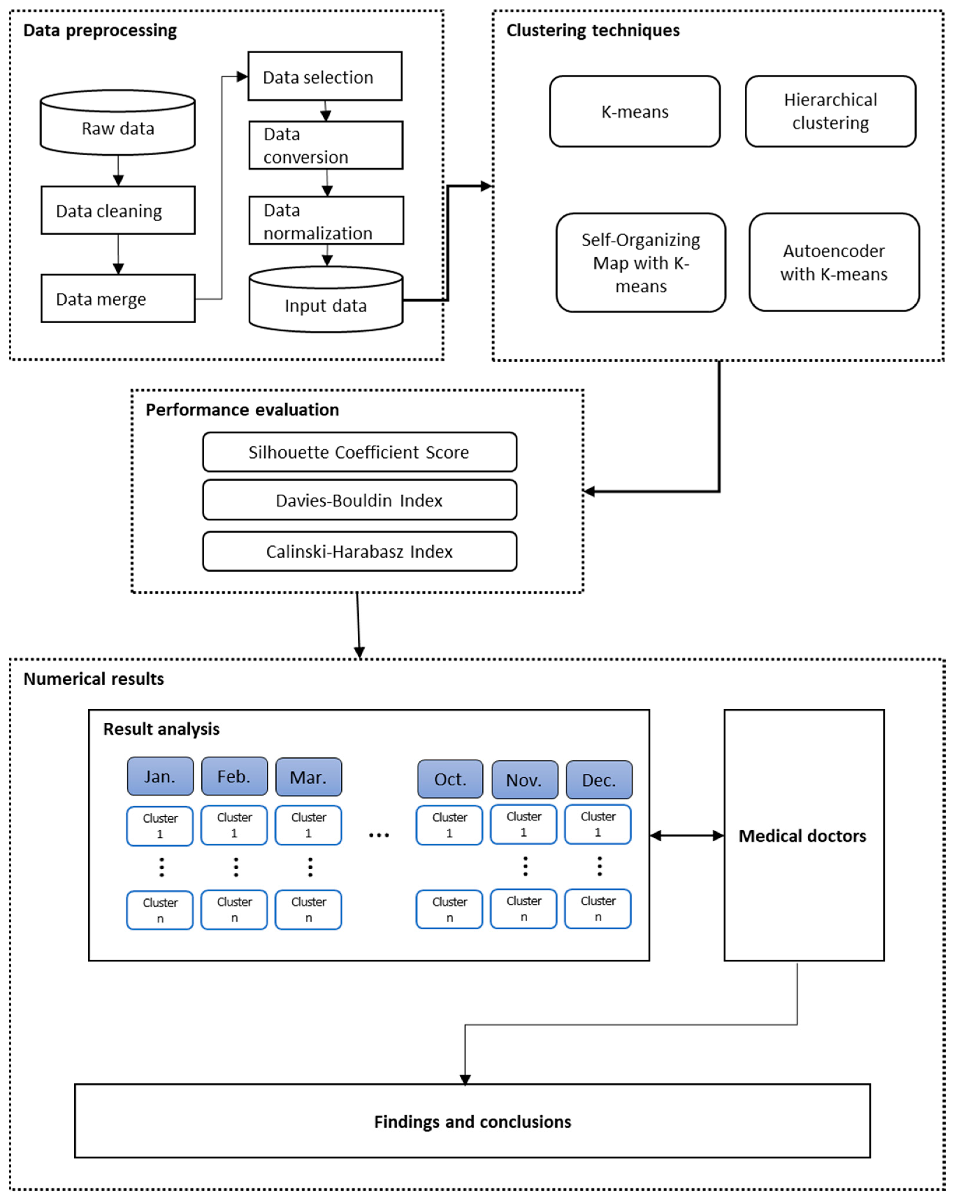
3. The Proposed SHCM System
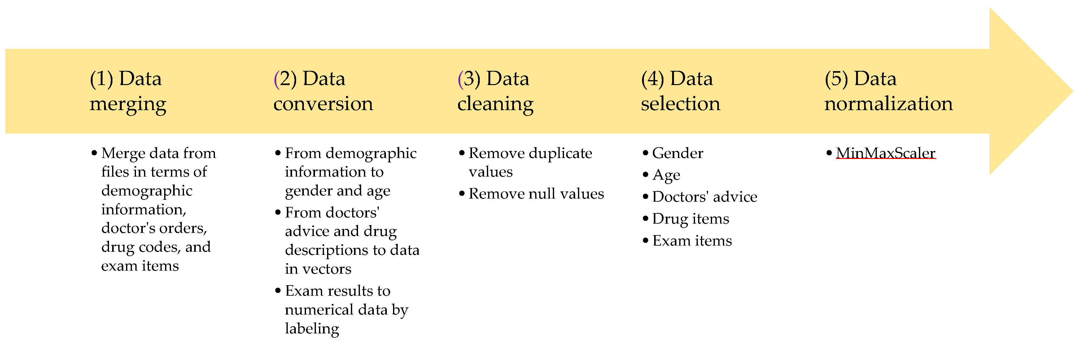
3.1. Data and Data Preprocessing
3.2. Performance Measurements
4. Numerical Results
4.1. Clustering Performance with Three Measurements
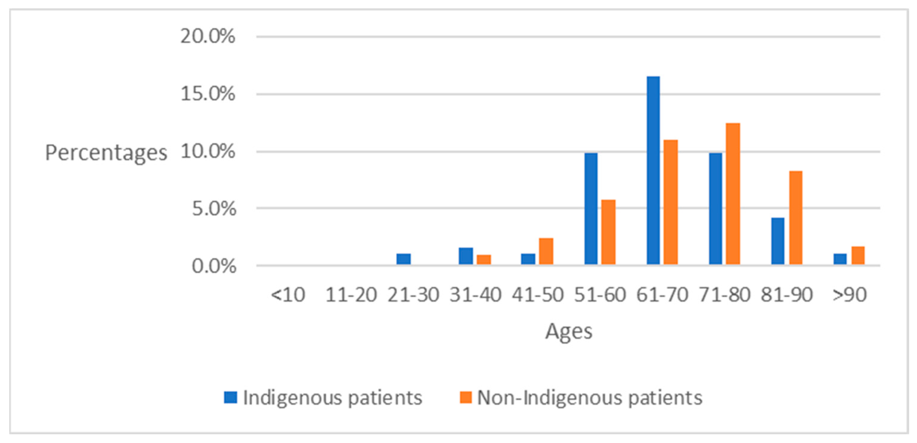
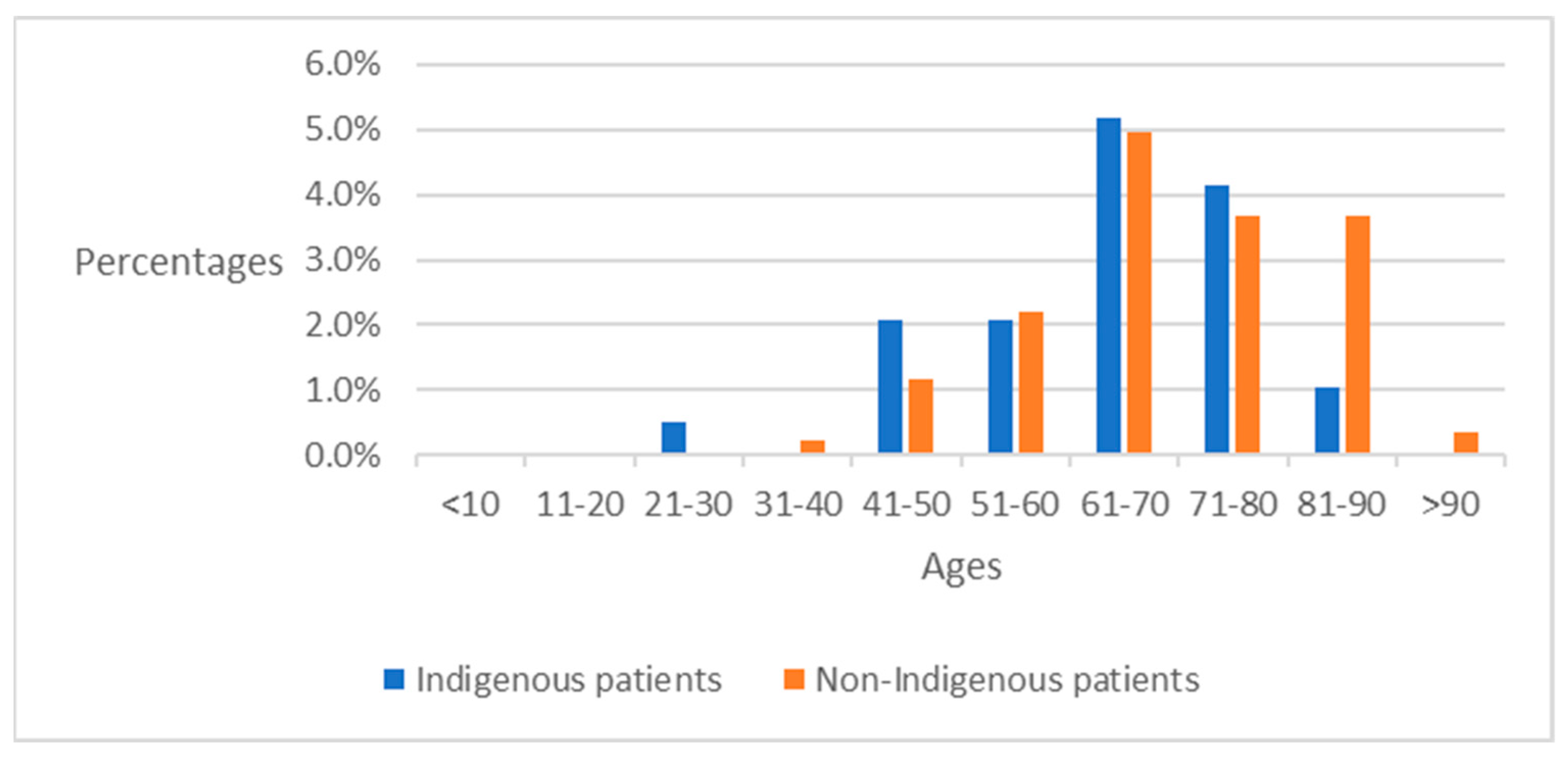
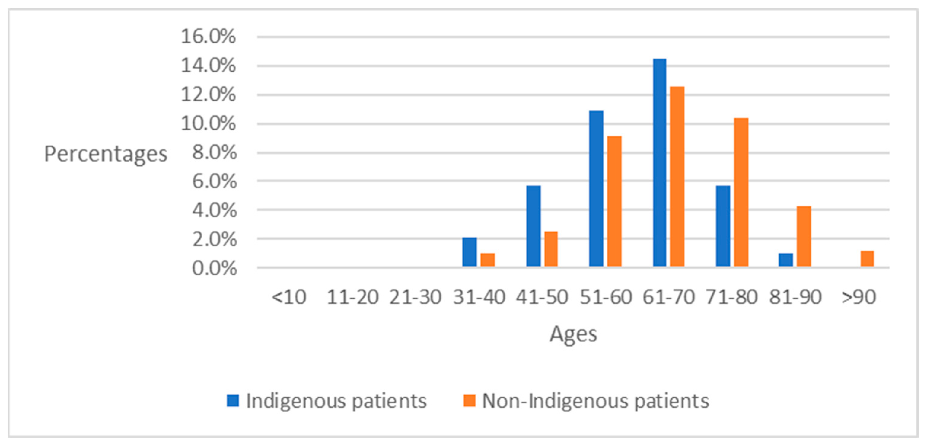
4.2. Preliminary Analysis of ICD-10-CM Codes between Indigenous Patients and Non-Indigenous Patients
4.3. Analysis of ICD-10-CM after Clustering
4.4. Analysis of Major Disease Codes over 12 Months in Indigenous Groups
4.5. Analysis of Major Disease Codes in Non-Indigenous Groups
4.6. Comparative Analysis of Major Disease Codes among Indigenous and Non-Indigenous Patients
4.6.1. Impacts of Infectious Diseases
4.6.2. Impacts of Type 2 Diabetes
4.6.3. Impacts of Essential Hypertension and Hypertensive Heart Diseases
5. Conclusions
Author Contributions
Funding
Institutional Review Board Statement
Informed Consent Statement
Data Availability Statement
Acknowledgments
Conflicts of Interest
Appendix A

| ICD-10 CM | Diseases |
|---|---|
| A09 | Infectious gastroenteritis and colitis, unspecified |
| B08 | Other viral infections characterized by skin and mucous membrane lesions, not elsewhere classified |
| B18 | Chronic viral hepatitis |
| C50 | Malignant neoplasm of breast |
| D64 | Other anemias |
| E11 | Type 2 diabetes mellitus |
| E78 | Disorders of lipoprotein metabolism and other lipidemias |
| E86 | Volume depletion |
| E87 | Other disorders of fluid, electrolyte and acid-base balance |
| G47 | Sleep disorders |
| I10 | Essential (primary) hypertension |
| I11 | Hypertensive heart disease |
| I20 | Angina pectoris |
| I25 | Chronic ischemic heart disease |
| I50 | Heart failure |
| J00 | Acute nasopharyngitis [common cold] |
| J01 | Acute sinusitis |
| J02 | Acute pharyngitis |
| J03 | Acute tonsillitis |
| J06 | Acute upper respiratory infections of multiple and unspecified sites |
| J12 | Viral pneumonia, not elsewhere classified |
| J18 | Pneumonia, unspecified organism |
| J20 | Acute bronchitis |
| J30 | Vasomotor and allergic rhinitis |
| J44 | Other chronic obstructive pulmonary disease |
| J45 | Asthma |
| K21 | Gastroesophageal reflux disease |
| K25 | Gastric ulcer |
| K29 | Gastritis and duodenitis |
| K59 | Other functional intestinal disorders |
| K92 | Other diseases of digestive system |
| L03 | Cellulitis and acute lymphangitis |
| L08 | Other local infections of skin and subcutaneous tissue |
| M10 | Gout |
| M19 | Other and unspecified osteoarthritis |
| M54 | Dorsalgia |
| N13 | Obstructive and reflux uropathy |
| N18 | Chronic kidney disease (CKD) |
| N20 | Calculus of kidney and ureter |
| N39 | Other disorders of urinary system |
| N40 | Benign prostatic hyperplasia |
| O47 | False labor |
| P59 | Neonatal jaundice from other and unspecified causes |
| R00 | Abnormalities of heart beat |
| R05 | Cough |
| R07 | Pain in throat and chest |
| R10 | Abdominal and pelvic pain |
| R11 | Nausea and vomiting |
| R31 | Hematuria |
| R35 | Polyuria |
| R42 | Dizziness and giddiness |
| R50 | Fever of other and unknown origin |
| R51 | Headache |
| R80 | Proteinuria |
| U07 | Emergency use of U07 |
| Z11 | Encounter for screening for infectious and parasitic diseases |
| Z20 | Contact with and (suspected) exposure to communicable diseases |
| Z34 | Encounter for supervision of normal pregnancy |
References
- Parimbelli, E.; Marini, S.; Sacchi, L.; Bellazzi, R. Patient similarity for precision medicine: A systematic review. J. Biomed. Inform. 2018, 83, 87–96. [Google Scholar] [CrossRef] [PubMed]
- Lambert, J.; Leutenegger, A.-L.; Jannot, A.-S.; Baudot, A. Tracking clusters of patients over time enables extracting information from medico-administrative databases. J. Biomed. Inform. 2023, 139, 104309. [Google Scholar] [CrossRef] [PubMed]
- Zelina, P.; Halámková, J.; Nováček, V. Unsupervised extraction, labelling and clustering of segments from clinical notes. In Proceedings of the 2022 IEEE International Conference on Bioinformatics and Biomedicine (BIBM), Las Vegas, NV, USA, 6–8 December 2022; pp. 1362–1368. [Google Scholar]
- Irving, J.; Patel, R.; Oliver, D.; Colling, C.; Pritchard, M.; Broadbent, M.; Baldwin, H.; Stahl, D.; Stewart, R.; Fusar-Poli, P. Using natural language processing on electronic health records to enhance detection and prediction of psychosis risk. Schizophr. Bull. 2021, 47, 405–414. [Google Scholar] [CrossRef] [PubMed]
- Ebad, S.A. Healthcare software design and implementation—A project failure case. Softw. Pract. Exp. 2020, 50, 1258–1276. [Google Scholar] [CrossRef]
- Mashoufi, M.; Ayatollahi, H.; Khorasani-Zavareh, D.; Talebi Azad Boni, T. Data quality in health care: Main concepts and assessment methodologies. Methods Inf. Med. 2023, 62, 005–018. [Google Scholar] [CrossRef] [PubMed]
- Ezugwu, A.E.; Ikotun, A.M.; Oyelade, O.O.; Abualigah, L.; Agushaka, J.O.; Eke, C.I.; Akinyelu, A.A. A comprehensive survey of clustering algorithms: State-of-the-art machine learning applications, taxonomy, challenges, and future research prospects. Eng. Appl. Artif. Intell. 2022, 110, 104743. [Google Scholar] [CrossRef]
- Saxena, A.; Prasad, M.; Gupta, A.; Bharill, N.; Patel, O.P.; Tiwari, A.; Er, M.J.; Ding, W.; Lin, C.-T. A review of clustering techniques and developments. Neurocomputing 2017, 267, 664–681. [Google Scholar] [CrossRef]
- Chaudhry, M.; Shafi, I.; Mahnoor, M.; Vargas, D.L.R.; Thompson, E.B.; Ashraf, I. A systematic literature review on identifying patterns using unsupervised clustering algorithms: A data mining perspective. Symmetry 2023, 15, 1679. [Google Scholar] [CrossRef]
- Oyewole, G.J.; Thopil, G.A. Data clustering: Application and trends. Artif. Intell. Rev. 2023, 56, 6439–6475. [Google Scholar] [CrossRef]
- Santamaría, L.P.; del Valle, E.P.G.; García, G.L.; Zanin, M.; González, A.R.; Ruiz, E.M.; Gallardo, Y.P.; Chan, G.S.H. Analysis of new nosological models from disease similarities using clustering. In Proceedings of the 2020 IEEE 33rd International Symposium on Computer-Based Medical Systems (CBMS), Rochester, MN, USA, 28–30 July 2020; pp. 183–188. [Google Scholar]
- Farouk, Y.; Rady, S. Early diagnosis of alzheimer’s disease using unsupervised clustering. Int. J. Intell. Comput. Inf. Sci. 2020, 20, 112–124. [Google Scholar] [CrossRef]
- Hassan, M.M.; Mollick, S.; Yasmin, F. An unsupervised cluster-based feature grouping model for early diabetes detection. Healthc. Anal. 2022, 2, 100112. [Google Scholar] [CrossRef]
- Antony, L.; Azam, S.; Ignatious, E.; Quadir, R.; Beeravolu, A.R.; Jonkman, M.; De Boer, F. A comprehensive unsupervised framework for chronic kidney disease prediction. IEEE Access 2021, 9, 126481–126501. [Google Scholar] [CrossRef]
- Enireddy, V.; Anitha, R.; Vallinayagam, S.; Maridurai, T.; Sathish, T.; Balakrishnan, E. Prediction of human diseases using optimized clustering techniques. Mater. Today Proc. 2021, 46, 4258–4264. [Google Scholar] [CrossRef]
- Arora, N.; Singh, A.; Al-Dabagh, M.Z.N.; Maitra, S.K. A novel architecture for diabetes patients’ prediction using k-means clustering and svm. Math. Probl. Eng. 2022, 2022, 4815521. [Google Scholar] [CrossRef]
- Parikh, H.M.; Remedios, C.L.; Hampe, C.S.; Balasubramanyam, A.; Fisher-Hoch, S.P.; Choi, Y.J.; Patel, S.; McCormick, J.B.; Redondo, M.J.; Krischer, J.P. Data mining framework for discovering and clustering phenotypes of atypical diabetes. J. Clin. Endocrinol. Metab. 2023, 108, 834–846. [Google Scholar] [CrossRef] [PubMed]
- Jasinska-Piadlo, A.; Bond, R.; Biglarbeigi, P.; Brisk, R.; Campbell, P.; Browne, F.; McEneaneny, D. Data-driven versus a domain-led approach to k-means clustering on an open heart failure dataset. Int. J. Data Sci. Anal. 2023, 15, 49–66. [Google Scholar] [CrossRef]
- Mpanya, D.; Celik, T.; Klug, E.; Ntsinjana, H. Clustering of heart failure phenotypes in johannesburg using unsupervised machine learning. Appl. Sci. 2023, 13, 1509. [Google Scholar] [CrossRef]
- Florensa, D.; Mateo-Fornés, J.; Solsona, F.; Pedrol Aige, T.; Mesas Julió, M.; Piñol, R.; Godoy, P. Use of multiple correspondence analysis and k-means to explore associations between risk factors and likelihood of colorectal cancer: Cross-sectional study. J. Med. Internet Res. 2022, 24, e29056. [Google Scholar] [CrossRef]
- Koné, A.P.; Scharf, D.; Tan, A. Multimorbidity and complexity among patients with cancer in ontario: A retrospective cohort study exploring the clustering of 17 chronic conditions with cancer. Cancer Control 2023, 30, 10732748221150393. [Google Scholar] [CrossRef]
- Chantraine, F.; Schreiber, C.; Pereira, J.A.C.; Kaps, J.; Dierick, F. Classification of stiff-knee gait kinematic severity after stroke using retrospective k-means clustering algorithm. J. Clin. Med. 2022, 11, 6270. [Google Scholar] [CrossRef]
- Yasa, I.; Rusjayanthi, N.; Luthfi, W.B.M. Classification of stroke using k-means and deep learning methods. Lontar Komput. J. Ilm. Teknol. Inf. 2022, 13, 23. [Google Scholar] [CrossRef]
- Al-Khafaji, H.M.R.; Jaleel, R.A. Adopting effective hierarchal iomts computing with k-efficient clustering to control and forecast covid-19 cases. Comput. Electr. Eng. 2022, 104, 108472. [Google Scholar] [CrossRef] [PubMed]
- Ilbeigipour, S.; Albadvi, A.; Noughabi, E.A. Cluster-based analysis of covid-19 cases using self-organizing map neural network and k-means methods to improve medical decision-making. Inform. Med. Unlocked 2022, 32, 101005. [Google Scholar] [CrossRef] [PubMed]
- MacQueen, J. Some methods for classification and analysis of multivariate observations. In Proceedings of the Fifth Berkeley Symposium on Mathematical Statistics and Probability, Berkeley, CA, USA, 18–21 June 1965 and 27 December 1965–7 January 1966; University of California Press: Oakland, CA, USA, 1967; pp. 281–297. [Google Scholar]
- Na, S.; Xumin, L.; Yong, G. Research on k-means clustering algorithm: An improved k-means clustering algorithm. In Proceedings of the 2010 Third International Symposium on Intelligent Information Technology and Security Informatics, Jian, China, 2–4 April 2010; pp. 63–67. [Google Scholar]
- Alam, M.S.; Rahman, M.M.; Hossain, M.A.; Islam, M.K.; Ahmed, K.M.; Ahmed, K.T.; Singh, B.C.; Miah, M.S. Automatic human brain tumor detection in mri image using template-based k means and improved fuzzy c means clustering algorithm. Big Data Cogn. Comput. 2019, 3, 27. [Google Scholar] [CrossRef]
- Lee, H.; Choi, Y.; Son, B.; Lim, J.; Lee, S.; Kang, J.W.; Kim, K.H.; Kim, E.J.; Yang, C.; Lee, J.-D. Deep autoencoder-powered pattern identification of sleep disturbance using multi-site cross-sectional survey data. Front. Med. 2022, 9, 950327. [Google Scholar] [CrossRef] [PubMed]
- Setiawan, K.E.; Kurniawan, A.; Chowanda, A.; Suhartono, D. Clustering models for hospitals in jakarta using fuzzy c-means and k-means. Procedia Comput. Sci. 2023, 216, 356–363. [Google Scholar] [CrossRef] [PubMed]
- Yuan, C.; Yang, H. Research on k-value selection method of k-means clustering algorithm. J 2019, 2, 226–235. [Google Scholar] [CrossRef]
- Murtagh, F.; Contreras, P. Algorithms for hierarchical clustering: An overview. Wiley Interdiscip. Rev. Data Min. Knowl. Discov. 2012, 2, 86–97. [Google Scholar] [CrossRef]
- Rumelhart, D.; Hinton, G.; Williams, R. Learning internal representations by error propagation. In Parallel Distributed Processing: Explorations in the Microstructure of Cognition; MIT Press: Cambridge, MA, USA, 1986; Chapter 8; Volume 1, pp. 318–362. [Google Scholar]
- Baldi, P. Autoencoders, unsupervised learning, and deep architectures. In Proceedings of the ICML Workshop on Unsupervised and Transfer Learning, Bellevue, WA, USA, 2 July 2011; JMLR Workshop and Conference Proceedings. ML Research Press: London, UK, 2012; pp. 37–49. [Google Scholar]
- Zhang, L.; Lv, C.; Jin, Y.; Cheng, G.; Fu, Y.; Yuan, D.; Tao, Y.; Guo, Y.; Ni, X.; Shi, T. Deep learning-based multi-omics data integration reveals two prognostic subtypes in high-risk neuroblastoma. Front. Genet. 2018, 9, 477. [Google Scholar] [CrossRef]
- Bank, D.; Koenigstein, N.; Giryes, R. Autoencoders. Machine Learning for Data Science Handbook: Data Mining and Knowledge Discovery Handbook; Springer: New York, NY, USA, 2023; pp. 353–374. [Google Scholar]
- Kohonen, T. The self-organizing map. Proc. IEEE 1990, 78, 1464–1480. [Google Scholar] [CrossRef]
- Vesanto, J.; Alhoniemi, E. Clustering of the self-organizing map. IEEE Trans. Neural Netw. 2000, 11, 586–600. [Google Scholar] [CrossRef] [PubMed]
- Caliński, T.; Harabasz, J. A dendrite method for cluster analysis. Commun. Stat.-Theory Methods 1974, 3, 1–27. [Google Scholar] [CrossRef]
- Desgraupes, B. Clustering indices. Univ. Paris Ouest-Lab Modal’X 2013, 1, 34. [Google Scholar]
- Davies, D.L.; Bouldin, D.W. A cluster separation measure. IEEE Trans. Pattern Anal. Mach. Intell. 1979, PAMI-1, 224–227. [Google Scholar] [CrossRef]
- Xiao, J.; Lu, J.; Li, X. Davies bouldin index based hierarchical initialization k-means. Intell. Data Anal. 2017, 21, 1327–1338. [Google Scholar] [CrossRef]
- Rousseeuw, P.J. Silhouettes: A graphical aid to the interpretation and validation of cluster analysis. J. Comput. Appl. Math. 1987, 20, 53–65. [Google Scholar] [CrossRef]
- Shahapure, K.R.; Nicholas, C. Cluster quality analysis using silhouette score. In Proceedings of the 2020 IEEE 7th International Conference on Data Science and Advanced Analytics (DSAA), Sydney, Australia, 6–9 October 2020; pp. 747–748. [Google Scholar]
- Harada, D.; Asanoi, H.; Noto, T.; Takagawa, J. Different pathophysiology and outcomes of heart failure with preserved ejection fraction stratified by k-means clustering. Front. Cardiovasc. Med. 2020, 7, 607760. [Google Scholar] [CrossRef]
| References | Years | Applications | Methods of Clustering |
|---|---|---|---|
| Santamaría et al. [11] | 2020 | Analysis of new nosological models | DBSCAN * |
| Farouk and Rady [12] | 2020 | Early diagnosis of Alzheimer’s disease | K-means, K-medoids |
| Hassan et al. [13] | 2022 | As a feature-grouping model for early diabetes detection | K-means |
| Antony et al. [14] | 2021 | Chronic kidney disease prediction | K-means, DBSCAN *, I-Forest *, Autoencoder |
| Enireddy et al. [15] | 2021 | Prediction of diseases | K-means, Agglomerative, Fuzzy C-means |
| Arora et al. [16] | 2022 | As a feature-extracted tool for diabetes patient prediction | K-means |
| Parikh et al. [17] | 2023 | Discovering and clustering phenotypes of atypical diabetes | K-means |
| Jasinska-Piadlo et al. [18] | 2023 | Clustering heart failures | K-means |
| Mpanya et al. [19] | 2023 | Clustering heart failure phenotypes | K-prototype, K-means, Agglomerative, BIRCH *, OPTICS *, DBSCAN *, GMM * |
| Florensa et al. [20] | 2022 | Exploring associations between risk factors and likelihood of colorectal cancer | K-means |
| Koné et al. [21] | 2023 | Exploring the clustering of 17 chronic conditions with cancer | K-means |
| Chantraine et al. [22] | 2022 | Classification of stiff-knee gait kinematic severity after stroke | K-means |
| Yasa et al. [23] | 2022 | Classification of stroke | K-means |
| Al-Khafaji and Jaleel [24] | 2022 | Controlling and forecasting COVID-19 cases | K-Efficient (a hybrid of K-medoids and K-means) |
| Ilbeigipour et al. [25] | 2022 | The analysis of COVID-19 cases | SOM, K-means |
| Variables | Attributes | Conversion Methods |
|---|---|---|
| X1 | Gender | Labeling |
| X2 | Age | From birthdays to ages |
| X3~X12 | Drug items | BERT and PCA |
| X13~X22 | Doctors’ advice | BERT and PCA |
| X23~Xn | Exam items | Labeling |
| Datasets | Jan. | Feb. | Mar. | Apr. | May | Jun. |
|---|---|---|---|---|---|---|
| Number of attributes | 456 | 394 | 418 | 447 | 417 | 416 |
| Visits of patients | 4765 | 4405 | 5667 | 5410 | 7593 | 5397 |
| Datasets | Jul. | Aug. | Sep. | Oct. | Nov. | Dec. |
| Number of attributes | 455 | 447 | 445 | 404 | 444 | 470 |
| Visits of patients | 5136 | 5341 | 5023 | 5233 | 4675 | 4506 |
| Methods | Jan. | Feb. | Mar. | Apr. | May | Jun. | Jul. | Aug. | Sep. | Oct. | Nov. | Dec. |
|---|---|---|---|---|---|---|---|---|---|---|---|---|
| KM | 4 | 4 | 3 | 3 | 5 | 3 | 3 | 3 | 3 | 3 | 3 | 3 |
| AEKM | 4 | 4 | 3 | 3 | 5 | 3 | 3 | 3 | 3 | 3 | 3 | 3 |
| SOMKM | 4 | 4 | 3 | 3 | 4 | 3 | 4 | 3 | 4 | 4 | 3 | 3 |
| HC | 4 | 4 | 3 | 3 | 3 | 3 | 3 | 3 | 3 | 3 | 3 | 4 |
| Methods | Jan. | Feb. | Mar. | Apr. | May | Jun. | Jul. | Aug. | Sep. | Oct. | Nov. | Dec. |
|---|---|---|---|---|---|---|---|---|---|---|---|---|
| KM | 1310.21 | 1431.42 | 1988.48 | 2107.83 | 1810.97 | 1892.51 | 1914.83 | 2082.41 | 1682.57 | 1731.59 | 1590.45 | 1323.84 |
| AEKM | 257.73 | 268.64 | 217.65 | 399.86 | 319.53 | 653.52 | 709.87 | 900.43 | 347.86 | 336.36 | 384.98 | 163.36 |
| SOMKM | 1281.33 | 1423.37 | 1988.48 | 1012.57 | 1377.30 | 1888.91 | 1432.10 | 1841.56 | 1391.69 | 1416.60 | 1590.45 | 1233.08 |
| HC | 1264.75 | 1368.76 | 1883.29 | 2008.26 | 2060.34 | 1847.02 | 1805.66 | 2035.00 | 1632.01 | 1690.22 | 1512.80 | 1112.01 |
| Methods | Jan. | Feb. | Mar. | Apr. | May | Jun. | Jul. | Aug. | Sep. | Oct. | Nov. | Dec. |
|---|---|---|---|---|---|---|---|---|---|---|---|---|
| KM | 1.43 | 1.28 | 1.43 | 1.25 | 1.6 | 1.31 | 1.27 | 1.28 | 1.44 | 1.5 | 1.35 | 1.58 |
| AEKM | 4.59 | 3.68 | 5.55 | 6 | 5.33 | 4.02 | 3.12 | 3.74 | 3.58 | 4.34 | 3.11 | 6.18 |
| SOMKM | 1.42 | 1.29 | 1.43 | 2.19 | 1.96 | 1.31 | 1.91 | 1.5 | 1.57 | 1.67 | 1.35 | 1.7 |
| HC | 1.45 | 1.31 | 1.43 | 1.27 | 1.49 | 1.32 | 1.34 | 1.28 | 1.43 | 1.52 | 1.38 | 1.53 |
| Methods | Jan. | Feb. | Mar. | Apr. | May | Jun. | Jul. | Aug. | Sep. | Oct. | Nov. | Dec. |
|---|---|---|---|---|---|---|---|---|---|---|---|---|
| KM | 0.27 | 0.29 | 0.27 | 0.32 | 0.24 | 0.31 | 0.31 | 0.32 | 0.27 | 0.25 | 0.29 | 0.23 |
| AEKM | 0.01 | 0.03 | 0.02 | 0.07 | 0.01 | 0.13 | 0.16 | 0.13 | 0.04 | 0.03 | 0.04 | 0.01 |
| SOMKM | 0.26 | 0.29 | 0.27 | 0.16 | 0.2 | 0.31 | 0.24 | 0.31 | 0.28 | 0.25 | 0.29 | 0.21 |
| HC | 0.27 | 0.29 | 0.25 | 0.31 | 0.26 | 0.3 | 0.3 | 0.32 | 0.26 | 0.25 | 0.29 | 0.25 |
| Ranks | Total | Cluster 1 | Cluster 2 | Cluster 3 | Cluster 4 | ||||||||||
|---|---|---|---|---|---|---|---|---|---|---|---|---|---|---|---|
| Codes | Disease % | Visits | Codes | Visits | Group % | Codes | Visits | Group % | Codes | Visits | Group % | Codes | Visits | Group % | |
| 1 | E11 | 9% | 178 | E11 | 87 | 49% | E11 | 24 | 13% | E11 | 62 | 35% | Z20 | 65 | 94% |
| 2 | E78 | 5% | 112 | I10 | 45 | 50% | E78 | 17 | 15% | E78 | 51 | 46% | J18 | 38 | 46% |
| 3 | I10 | 4% | 90 | E78 | 44 | 39% | N39 | 17 | 50% | I11 | 28 | 35% | J01 | 16 | 36% |
| 4 | J18 | 4% | 82 | I11 | 43 | 53% | I10 | 16 | 18% | I10 | 27 | 30% | R50 | 14 | 45% |
| 5 | I11 | 4% | 81 | J18 | 22 | 27% | N18 | 12 | 32% | I25 | 21 | 45% | E11 | 5 | 3% |
| 6 | Z20 | 3% | 69 | B18 | 22 | 55% | R50 | 10 | 32% | M10 | 20 | 65% | J20 | 5 | 18% |
| 7 | I25 | 2% | 47 | K21 | 21 | 54% | I11 | 9 | 11% | B18 | 17 | 43% | J45 | 5 | 17% |
| 8 | J01 | 2% | 44 | Z34 | 18 | 60% | Z34 | 8 | 27% | J18 | 16 | 20% | R10 | 5 | 19% |
| 9 | B18 | 2% | 40 | I25 | 15 | 32% | I25 | 7 | 15% | J01 | 15 | 34% | I25 | 4 | 9% |
| 10 | K21 | 2% | 39 | J45 | 14 | 48% | R10 | 7 | 26% | K21 | 14 | 36% | N18 | 4 | 11% |
| 11 | N18 | 2% | 37 | N20 | 7 | 47% | J30 | 4 | 17% | ||||||
| 12 | N39 | 2% | 34 | M10 | 6 | 19% | A09 | 4 | 21% | ||||||
| 13 | R50 | 2% | 31 | J18 | 6 | 7% | R11 | 4 | 31% | ||||||
| 14 | M10 | 2% | 31 | E86 | 4 | 50% | |||||||||
| 15 | Z34 | 1% | 30 | Z34 | 4 | 13% | |||||||||
| Ranks | Total | Cluster 1 | Cluster 2 | Cluster 3 | ||||||||
|---|---|---|---|---|---|---|---|---|---|---|---|---|
| Codes | Disease % | Visits | Codes | Visits | Group % | Codes | Visits | Group % | Codes | Visits | Group % | |
| 1 | E11 | 8% | 206 | E11 | 30 | 15% | E11 | 93 | 45% | E11 | 83 | 40% |
| 2 | E78 | 6% | 154 | R50 | 25 | 45% | Z20 | 79 | 74% | E78 | 63 | 41% |
| 3 | I10 | 4% | 108 | N39 | 23 | 56% | E78 | 69 | 45% | I10 | 36 | 33% |
| 4 | Z20 | 4% | 107 | E78 | 22 | 14% | I10 | 55 | 51% | I11 | 34 | 34% |
| 5 | I11 | 4% | 99 | I10 | 17 | 16% | I11 | 53 | 54% | Z11 | 33 | 60% |
| 6 | J18 | 3% | 80 | N18 | 14 | 25% | J18 | 41 | 51% | J01 | 31 | 41% |
| 7 | J01 | 3% | 76 | I11 | 12 | 12% | J01 | 39 | 51% | M10 | 30 | 60% |
| 8 | B18 | 2% | 56 | J18 | 12 | 15% | K21 | 29 | 63% | Z20 | 28 | 26% |
| 9 | R50 | 2% | 56 | R10 | 11 | 35% | Z34 | 28 | 82% | J18 | 27 | 34% |
| 10 | N18 | 2% | 56 | I25 | 9 | 20% | B18 | 26 | 46% | B18 | 26 | 46% |
| 11 | Z11 | 2% | 55 | N18 | 26 | 46% | ||||||
| 12 | M10 | 2% | 50 | |||||||||
| 13 | K21 | 2% | 46 | |||||||||
| 14 | I25 | 2% | 46 | |||||||||
| 15 | N39 | 2% | 41 | |||||||||
| Ranks | Total | Cluster 1 | Cluster 2 | Cluster 3 | Cluster 4 | Cluster 5 | ||||||||||||
|---|---|---|---|---|---|---|---|---|---|---|---|---|---|---|---|---|---|---|
| Codes | Disease % | Visits | Codes | Visits | Group % | Codes | Visits | Group % | Codes | Visits | Group % | Codes | Visits | Group % | Codes | Visits | Group % | |
| 1 | Z20 | 22% | 660 | E11 | 58 | 35% | E11 | 83 | 50% | Z20 | 240 | 36% | N39 | 23 | 62% | Z20 | 346 | 52% |
| 2 | E11 | 6% | 167 | E78 | 46 | 43% | Z20 | 56 | 8% | R05 | 56 | 45% | R50 | 21 | 22% | R05 | 66 | 53% |
| 3 | R05 | 4% | 125 | I11 | 27 | 34% | E78 | 49 | 45% | J06 | 30 | 37% | E11 | 21 | 13% | U07 | 40 | 48% |
| 4 | E78 | 4% | 108 | B18 | 20 | 47% | I10 | 40 | 61% | R50 | 29 | 31% | I11 | 12 | 15% | J06 | 39 | 48% |
| 5 | R50 | 3% | 94 | I10 | 19 | 29% | I11 | 38 | 48% | U07 | 25 | 30% | E78 | 11 | 10% | R50 | 29 | 31% |
| 6 | U07 | 3% | 83 | K21 | 14 | 42% | Z34 | 30 | 65% | J18 | 10 | 19% | N18 | 10 | 20% | J18 | 9 | 17% |
| 7 | J06 | 3% | 81 | J44 | 14 | 61% | I25 | 23 | 50% | J20 | 10 | 33% | Z34 | 9 | 20% | J00 | 8 | 50% |
| 8 | I11 | 3% | 79 | Z20 | 13 | 2% | B18 | 20 | 47% | J00 | 8 | 50% | N40 | 9 | 64% | Z34 | 7 | 15% |
| 9 | I10 | 2% | 66 | J18 | 13 | 24% | N18 | 20 | 41% | J01 | 7 | 39% | I25 | 7 | 15% | J20 | 7 | 23% |
| 10 | J18 | 2% | 54 | N18 | 12 | 24% | K21 | 18 | 55% | N18 | 6 | 12% | M10 | 7 | 24% | R10 | 5 | 23% |
| 11 | N18 | 2% | 49 | I25 | 12 | 26% | J18 | 16 | 30% | J30 | 5 | 26% | I10 | 7 | 11% | J02 | 5 | 63% |
| 12 | Z34 | 2% | 46 | M10 | 12 | 41% | E11 | 4 | 2% | J18 | 6 | 11% | ||||||
| 13 | I25 | 2% | 46 | I25 | 4 | 9% | N20 | 6 | 55% | |||||||||
| 14 | B18 | 1% | 43 | R51 | 4 | 20% | R10 | 6 | 27% | |||||||||
| 15 | N39 | 1% | 37 | R11 | 4 | 27% | M54 | 6 | 30% | |||||||||
| Ranks | Total | Cluster 1 | Cluster 2 | Cluster 3 | ||||||||
|---|---|---|---|---|---|---|---|---|---|---|---|---|
| Codes | Disease % | Visits | Codes | Visits | Group % | Codes | Visits | Group % | Codes | Visits | Group % | |
| 1 | Z20 | 15% | 309 | E11 | 58 | 40% | E11 | 83 | 57% | Z20 | 240 | 78% |
| 2 | E11 | 7% | 145 | E78 | 46 | 47% | Z20 | 56 | 18% | R05 | 56 | 95% |
| 3 | E78 | 5% | 97 | I11 | 27 | 40% | E78 | 49 | 51% | J06 | 30 | 75% |
| 4 | I11 | 3% | 67 | B18 | 20 | 50% | I10 | 40 | 68% | R50 | 29 | 66% |
| 5 | I10 | 3% | 59 | I10 | 19 | 32% | I11 | 38 | 57% | U07 | 25 | 64% |
| 6 | R05 | 3% | 59 | K21 | 14 | 44% | Z34 | 30 | 100% | J18 | 10 | 26% |
| 7 | R50 | 2% | 44 | J44 | 14 | 78% | I25 | 23 | 59% | J20 | 10 | 56% |
| 8 | B18 | 2% | 40 | Z20 | 13 | 4% | B18 | 20 | 50% | J00 | 8 | 100% |
| 9 | J06 | 2% | 40 | J18 | 13 | 33% | N18 | 20 | 53% | J01 | 7 | 44% |
| 10 | J18 | 2% | 39 | I25 | 12 | 31% | K21 | 18 | 56% | N18 | 6 | 16% |
| 11 | I25 | 2% | 39 | N18 | 12 | 32% | J18 | 16 | 41% | J30 | 5 | 33% |
| 12 | U07 | 2% | 39 | M10 | 12 | 55% | E11 | 4 | 3% | |||
| 13 | N18 | 2% | 38 | Z11 | 11 | 48% | I25 | 4 | 10% | |||
| 14 | K21 | 2% | 32 | K25 | 11 | 50% | R51 | 4 | 24% | |||
| 15 | Z34 | 1% | 30 | R50 | 9 | 20% | R11 | 4 | 40% | |||
| Ranks | Total | Cluster 1 | Cluster 2 | Cluster 3 | Cluster 4 | ||||||||||
|---|---|---|---|---|---|---|---|---|---|---|---|---|---|---|---|
| Codes | Disease % | Visits | Codes | Visits | Group % | Codes | Visits | Group % | Codes | Visits | Group % | Codes | Visits | Group % | |
| 1 | E11 | 8% | 985 | E11 | 364 | 37% | E11 | 176 | 18% | E11 | 414 | 42% | Z20 | 412 | 96% |
| 2 | E78 | 6% | 790 | E78 | 316 | 40% | N39 | 135 | 73% | E78 | 349 | 44% | J18 | 50 | 32% |
| 3 | I11 | 5% | 680 | I11 | 303 | 45% | E78 | 121 | 15% | I11 | 286 | 42% | E11 | 31 | 3% |
| 4 | Z20 | 3% | 429 | I10 | 149 | 38% | N18 | 81 | 20% | I10 | 169 | 43% | N18 | 30 | 7% |
| 5 | N18 | 3% | 407 | N18 | 142 | 35% | I11 | 80 | 12% | N18 | 154 | 38% | R50 | 21 | 24% |
| 6 | I10 | 3% | 391 | K21 | 109 | 51% | N20 | 72 | 51% | I25 | 114 | 48% | J01 | 18 | 21% |
| 7 | I25 | 2% | 237 | B18 | 88 | 43% | I10 | 59 | 15% | B18 | 104 | 51% | I10 | 14 | 4% |
| 8 | K21 | 2% | 212 | G47 | 88 | 55% | N40 | 54 | 42% | K21 | 89 | 42% | R10 | 14 | 11% |
| 9 | B18 | 2% | 204 | I25 | 82 | 35% | R10 | 44 | 34% | M10 | 77 | 66% | K92 | 13 | 21% |
| 10 | N39 | 1% | 184 | K59 | 68 | 46% | R50 | 35 | 41% | N40 | 72 | 55% | A09 | 13 | 19% |
| 11 | G47 | 1% | 161 | I25 | 30 | 13% | E86 | 13 | 24% | ||||||
| 12 | J18 | 1% | 158 | Z34 | 26 | 28% | |||||||||
| 13 | K59 | 1% | 147 | R31 | 25 | 78% | |||||||||
| 14 | N20 | 1% | 140 | ||||||||||||
| 15 | N40 | 1% | 130 | ||||||||||||
| Ranks | Total | Cluster 1 | Cluster 2 | Cluster 3 | ||||||||
|---|---|---|---|---|---|---|---|---|---|---|---|---|
| Codes | Disease % | Visits | Codes | Visits | Group % | Codes | Visits | Group % | Codes | Visits | Group % | |
| 1 | E11 | 7% | 953 | N39 | 177 | 71% | E11 | 406 | 43% | E11 | 393 | 41% |
| 2 | E78 | 6% | 827 | E11 | 154 | 16% | Z20 | 394 | 58% | E78 | 351 | 42% |
| 3 | I11 | 5% | 676 | E78 | 109 | 13% | E78 | 367 | 44% | I11 | 284 | 42% |
| 4 | Z20 | 5% | 674 | N18 | 103 | 23% | I11 | 313 | 46% | Z20 | 280 | 42% |
| 5 | I10 | 3% | 464 | I11 | 79 | 12% | I10 | 184 | 40% | I10 | 210 | 45% |
| 6 | N18 | 3% | 450 | R50 | 75 | 50% | N18 | 154 | 34% | N18 | 193 | 43% |
| 7 | I25 | 2% | 283 | I10 | 70 | 15% | G47 | 111 | 60% | I25 | 156 | 55% |
| 8 | N39 | 2% | 251 | R10 | 58 | 43% | K21 | 104 | 49% | J44 | 106 | 70% |
| 9 | K21 | 1% | 213 | N20 | 47 | 38% | I25 | 98 | 35% | J18 | 105 | 53% |
| 10 | J18 | 1% | 199 | N40 | 36 | 27% | K59 | 80 | 53% | B18 | 100 | 54% |
| 11 | B18 | 1% | 186 | M10 | 32 | 26% | Z34 | 78 | 71% | N40 | 97 | 73% |
| 12 | G47 | 1% | 186 | Z34 | 32 | 29% | J18 | 78 | 39% | K21 | 95 | 45% |
| 13 | J44 | 1% | 152 | R31 | 30 | 70% | J30 | 76 | 51% | M10 | 72 | 58% |
| 14 | K59 | 1% | 151 | I25 | 29 | 10% | N20 | 66 | 53% | |||
| 15 | R50 | 1% | 151 | |||||||||
| Ranks | Total | Cluster 1 | Cluster 2 | Cluster 3 | Cluster 4 | Cluster 5 | ||||||||||||
|---|---|---|---|---|---|---|---|---|---|---|---|---|---|---|---|---|---|---|
| Codes | Disease % | Visits | Codes | Visits | Group % | Codes | Visits | Group % | Codes | Visits | Group % | Codes | Visits | Group % | Codes | Visits | Group % | |
| 1 | Z20 | 19% | 2922 | E11 | 367 | 41% | E11 | 354 | 40% | Z20 | 1029 | 35% | E11 | 151 | 17% | Z20 | 1343 | 46% |
| 2 | E11 | 6% | 888 | E78 | 311 | 42% | Z20 | 325 | 11% | R05 | 242 | 44% | N39 | 131 | 72% | R05 | 301 | 54% |
| 3 | E78 | 5% | 740 | I11 | 285 | 44% | E78 | 308 | 42% | U07 | 129 | 37% | E78 | 111 | 15% | U07 | 153 | 43% |
| 4 | I11 | 4% | 648 | Z20 | 212 | 7% | I11 | 279 | 43% | J06 | 120 | 45% | N18 | 92 | 22% | J06 | 111 | 42% |
| 5 | R05 | 4% | 553 | N18 | 171 | 41% | I10 | 149 | 39% | R50 | 88 | 31% | I11 | 78 | 12% | R50 | 75 | 27% |
| 6 | N18 | 3% | 420 | I10 | 156 | 41% | N18 | 138 | 33% | J00 | 38 | 54% | R50 | 73 | 26% | J00 | 31 | 44% |
| 7 | I10 | 2% | 382 | I25 | 109 | 44% | K21 | 102 | 55% | R11 | 16 | 29% | I10 | 62 | 16% | Z34 | 20 | 16% |
| 8 | U07 | 2% | 352 | N40 | 84 | 64% | I25 | 101 | 41% | J20 | 16 | 29% | N20 | 48 | 44% | J20 | 16 | 29% |
| 9 | R50 | 2% | 281 | B18 | 78 | 49% | G47 | 87 | 54% | E11 | 14 | 2% | N40 | 43 | 33% | R11 | 13 | 24% |
| 10 | J06 | 2% | 265 | K21 | 72 | 39% | Z34 | 79 | 64% | N18 | 14 | 3% | R10 | 32 | 31% | R07 | 11 | 16% |
| 11 | I25 | 2% | 248 | B18 | 74 | 46% | R35 | 30 | 67% | J03 | 10 | 34% | ||||||
| 12 | K21 | 1% | 186 | C50 | 58 | 91% | R51 | 10 | 25% | |||||||||
| 13 | N39 | 1% | 181 | K25 | 55 | 54% | O47 | 10 | 77% | |||||||||
| 14 | G47 | 1% | 162 | R00 | 54 | 62% | ||||||||||||
| 15 | B18 | 1% | 160 | |||||||||||||||
| Ranks | Total | Cluster 1 | Cluster 2 | Cluster 3 | ||||||||
|---|---|---|---|---|---|---|---|---|---|---|---|---|
| Codes | Disease % | Visits | Codes | Visits | Group % | Codes | Visits | Group % | Codes | Visits | Group % | |
| 1 | Z20 | 11% | 1440 | Z20 | 867 | 60% | Z20 | 558 | 39% | E11 | 140 | 17% |
| 2 | E11 | 6% | 822 | E11 | 342 | 42% | E11 | 340 | 41% | N39 | 111 | 66% |
| 3 | E78 | 5% | 681 | E78 | 294 | 43% | E78 | 285 | 42% | E78 | 102 | 15% |
| 4 | I11 | 5% | 588 | I11 | 259 | 44% | I11 | 250 | 43% | N18 | 89 | 22% |
| 5 | N18 | 3% | 399 | N18 | 147 | 37% | I10 | 165 | 45% | I11 | 79 | 13% |
| 6 | I10 | 3% | 365 | I10 | 145 | 40% | N18 | 163 | 41% | R50 | 69 | 29% |
| 7 | U07 | 2% | 267 | U07 | 124 | 46% | I25 | 115 | 54% | I10 | 55 | 15% |
| 8 | R50 | 2% | 238 | Z34 | 102 | 83% | U07 | 106 | 40% | U07 | 37 | 14% |
| 9 | I25 | 2% | 214 | I25 | 80 | 37% | J44 | 96 | 69% | N20 | 37 | 44% |
| 10 | N39 | 1% | 168 | G47 | 77 | 53% | R50 | 93 | 39% | R10 | 31 | 34% |
| 11 | B18 | 1% | 148 | J18 | 74 | 54% | N40 | 26 | 27% | |||
| 12 | K21 | 1% | 147 | M10 | 71 | 63% | R31 | 25 | 86% | |||
| 13 | G47 | 1% | 145 | N40 | 70 | 73% | ||||||
| 14 | J06 | 1% | 143 | B18 | 67 | 45% | ||||||
| 15 | J44 | 1% | 140 | K21 | 65 | 44% | ||||||
| Months | Clusters of Indigenous Patients | Clusters of Non-Indigenous Patients | ||||||||
|---|---|---|---|---|---|---|---|---|---|---|
| Class A | Class B | Class C | Class D | Class E | Class A | Class B | Class C | Class D | Class E | |
| Jan. | I10, I11, B18, K21, Z34 | N39 | M10 | Z20, E86 | K21, G47 | N39, N20, R31 | B18, M10, N40 | Z20 | ||
| Feb. | E78, Z34, I25, K21, J45, G47, M19 | N39, N20 | M10, B18, Z11 | Z20, R07, L08, B08 | G47, Z34 | N39 | B18, N40, M10 | Z20 | ||
| Mar. | E11, I10, I11, J18, J01, K21, Z34 | N39 | Z11, M10 | Z20, G47, K59, Z34, J30 | N39, R50, R31 | I25, J44, J18, B18, N40, M10, N20 | ||||
| Apr. | Z20, I11, K21, Z34, B18 | N39, N20 | J01, N18, Z11 | Z20, K21, G47, Z34, C50 | N39, R35 | I25, B18, J44, J18, M10, N40, K25, I20 | ||||
| May | E11, E78, I10, I11, Z34, I25, B18, N18, K21 | N39, Z34, N20 | E78, B18, K21, J44, M10 | Z20, R05, U07, J06, J00, J02 | J00, R05 | E78, I11, K21, I25, G47, Z34, B18, C50, K25, R00 | N39, N20, R35 | E11, E78, I11, N18, I10, I25, N40, B18 | Z20, R05, U07, J06, J00, O47 | J00, R05, J06 |
| Jun. | E11, E78, I10, I11, Z34, I25, B18, N18, K21 | B18, J44, M10, K25 | Z20, R05, J06, R50, U07, J20, J00 | Z20, Z34, G47 | N39, R31 | I25, J44, J18, M10, N40 | ||||
| Jul. | Z20, E11, E78, I11, I10, Z34, K21, B18 | N20 | M10 | Z20, Z34, K21, G47, K59, R42, R00 | N39 | I25, B18, J44, N40, J18, M10 | ||||
| Aug. | Z20, E11, E78, I10, I11, Z34, K21, J01, B18, J20, K59 | N39 | J18, I25, M10, J44 | Z20, K21, Z34 | N39, R31 | I25, B18, J44, N40, M10, J18 | ||||
| Sep. | Z20, E78, I11, B18, K21, Z34 | N39 | J18, M10 | Z20, Z34, K21, K59, G47, R42 | N39, R31 | I25, B18, J19, N40, J44, M10 | ||||
| Oct. | E11, Z20, I11, K21, Z34, J45 | N39, R10, N13 | R50, J18, M10, N18, J20, J01, J06 | Z20, Z34, G47 | N39, N20, R31 | R50, N18, J18, Z20, I25, B18, U07, J20, M10, N40 | ||||
| Nov. | I10, Z34, J12, Z20, P59 | N39 | J18, M10, J45, J20 | Z34, K21, R42, Z20, G47 | N39, R31, R80 | J18, I25, J44, B18, N40 | ||||
| Dec. | E11, I10, I11, K21, P59, J45, Z34, J20, J30 | N39, R10, N20, J03 | J18, M10 | Z34, G47, K59, C50, R42 | N39, R31, R35 | I25, J18, J44, M10, N40, I20 | ||||
| SAME CODE | I10, I11, K21, Z34 | N39 | M10 | Z20 | J00 | K21, G47 | N39 | M10, N40 | Z20 | J00 |
Disclaimer/Publisher’s Note: The statements, opinions and data contained in all publications are solely those of the individual author(s) and contributor(s) and not of MDPI and/or the editor(s). MDPI and/or the editor(s) disclaim responsibility for any injury to people or property resulting from any ideas, methods, instructions or products referred to in the content. |
© 2023 by the authors. Licensee MDPI, Basel, Switzerland. This article is an open access article distributed under the terms and conditions of the Creative Commons Attribution (CC BY) license (https://creativecommons.org/licenses/by/4.0/).
Share and Cite
Yang, W.-C.; Lai, J.-P.; Liu, Y.-H.; Lin, Y.-L.; Hou, H.-P.; Pai, P.-F. Using Medical Data and Clustering Techniques for a Smart Healthcare System. Electronics 2024, 13, 140. https://doi.org/10.3390/electronics13010140
Yang W-C, Lai J-P, Liu Y-H, Lin Y-L, Hou H-P, Pai P-F. Using Medical Data and Clustering Techniques for a Smart Healthcare System. Electronics. 2024; 13(1):140. https://doi.org/10.3390/electronics13010140
Chicago/Turabian StyleYang, Wen-Chieh, Jung-Pin Lai, Yu-Hui Liu, Ying-Lei Lin, Hung-Pin Hou, and Ping-Feng Pai. 2024. "Using Medical Data and Clustering Techniques for a Smart Healthcare System" Electronics 13, no. 1: 140. https://doi.org/10.3390/electronics13010140
APA StyleYang, W.-C., Lai, J.-P., Liu, Y.-H., Lin, Y.-L., Hou, H.-P., & Pai, P.-F. (2024). Using Medical Data and Clustering Techniques for a Smart Healthcare System. Electronics, 13(1), 140. https://doi.org/10.3390/electronics13010140