Abstract
Automatic modulation classification (AMC) using convolutional neural networks (CNNs) is an active area of research that has the potential to improve the efficiency and reliability of wireless communication systems significantly. AMC is the approach used in a communication system to detect the type of modulation format at the receiver end. This paper proposes a voting-based deep convolutional neural network (VB-DCNN) for classifying M-QAM and M-PSK signals. M-QAM and M-PSK signal waveforms are generated and passed through the fading channel in the presence of additive white Gaussian noise (AWGN). The VB-DCNN extracts features from the input signal through convolutional layers, and classification is performed on these features. Multiple network instances are trained on different subsets of training data in the VB-DCNN. A network instance predicts the input signal during testing. Based on the votes, the final prediction is made. Different simulation experiments are carried out to analyze the performance of the trained network, and the DCNN is designed with the Deep Neural Network Toolbox in MATLAB. The generated frames are divided into training, validation, and test datasets. Lastly, the classification accuracy of the trained network is determined using test frames. The proposed model’s accuracy is near to 100% at lower SNRs. The simulation results show the superiority of the proposed VB-DCNN compared to existing state-of-the-art techniques.
1. Introduction
AMC has many applications in military, civilian, software-defined radio, cognitive radio network, and smart grid communication [1]. Recent advances in wireless communication, such as wireless power mobile edge cloud computing, have created new study gaps, allowing academics to explore the issue of AMC [2]. AMC has been employed in multiple-input multiple-output (MIMO) systems and deep learning methods [3,4,5]. AMC may be explored further for the application era of nonorthogonal multiple access (NOMA) and in 6G communication [6,7].
Signal processing and analysis can only be conducted when the received signal’s modulation format is recognized. For example, by recognizing the modulation type of the received signal in a software-defined radio (SDR)-based communication system, the receiver can demodulate the received signal through a demodulation algorithm [8]. So, the transmitted signal does not need to contain additional control information for informing the receiver, which is helpful to lessen the procedure overhead. AMC is broadly divided into two approaches:
- The likelihood function-based decision-theoretic (DT) approach;
- The features-based pattern recognition (PR) approach.
In the DT approach, the received signal likelihood function is evaluated. Various likelihood ratio tests (LRTs) have been employed, such as average, generalized, hybrid, and many more. In the PR approach, there are two phases: in the first phase, various parameters have been extracted from the received signal, and distinct features have been selected. In the second phase, the features are fed into the classifier structure for classifying modulation formats [9].
Due to the superior performance of the CNN in feature extraction, it is used for modulation classification. Another advantage of the CNN model is that it requires minimal pre-processing. CNNs can achieve higher accuracy than traditional expert feature engineering. In many traditional pattern recognition methods, it is necessary to manually extract signal features, such as instantaneous statistics, high-order statistics, time-frequency characteristics, asynchronous delay sampling characteristics, etc. These features are inputs to the classifier, such as decision trees. The support vector classifier uses these features as inputs, such as decision trees and support vector machines. Though simple with less computation, it shows poor performance for nonlinear problems. The CNN has a multi-layer structure, which can better extract features of the signal, avoiding the tedious manual selection of data features [10].
This research aims to automatically classify the received modulated signals using a convolution neural network. In the first step, signals of several modulations are generated by simulation and transmitted through an AWGN channel. The problem is classifying the modulated signals at the receiver end using the CNN. In the second step, the CNN is trained using the generated waveforms as training data. Then, the trained network is assessed by obtaining the classification accuracy of the test frames.
1.1. Contribution of This Paper
The contributions of the proposed modulation classification scheme are as follows:
- The major goal is to automatically classify modulated signals using a voting-based deep convolutional neural network (VB-DCNN).
- The VB-DCNN does not require prior knowledge of the symbol rate or baud rate. Therefore, it reduces the testing framework’s execution requirements, improving classification and processing efficiency.
- In the VB-DCNN, the size of the input signal is fixed for classification, but the length of the actual signal is flexible. It is intended to use the complete input signal burst to increase classification accuracy further.
1.2. Organization of This Paper
This paper is organized as follows: Section 2 demonstrates the proposed system model of the received signal. Section 3 describes the VB-DCNN for the classification of modulation formats. The deep network design, CNN layers, and basic principles of the proposed voting-based fusion are comprehensively explained in this section. The performance of the VB-DCNN is evaluated in Section 4 on various fading channels and for different numbers of DCNN layers. Three different cases are considered to evaluate the classifier’s performance. The paper is concluded in Section 5.
2. Related Work
Recently, deep-learning-based approaches have been proposed for modulation classification in [11,12]. The deep residual network and long short-term memory (LSTM) are employed for modulation classification in [13]. The authors used two CNN models for modulation classification, i.e., AlexNet and GoogleNet [14]. In [15], the authors present an adaptive visibility graph (AVG) algorithm that can adaptively map time series into graphs, establishing an end-to-end modulation classification framework.
For the application of radar signals, especially in electronic reconnaissance, the authors in [16] presented the detecting radiation signals under an intense noise background using an X-shaped structure, i.e., X-net. For the classification of the training dataset, which is distributed over a network without gathering the data at a centralized location, the authors in [17] presented the decentralized-learning-based AMC (DecentAMC) along with the regularized-modulation classification network (R-MCNet) and an innovative learning framework (DeEnAMC).
In [18], cumulants and a blind channel estimation multi-classification algorithm based on maximum likelihood is used to classify modulated signals. In [19], the K-nearest neighbor algorithm and genetic programming are chosen for classifying certain modulated signals. In [20], the authors compared the performance of different neural network models and lowered the training complexity by lowering the input signal dimension. To improve the efficiency of training CNNs, the authors in [21] proposed a two-step training method.
The authors proposed a denoising autoencoder classifier based on LSTM in [22] that achieved higher accuracy at higher SNRs. The work of a CLDNN with CNN and LSTM cascaded together [23] presents a CNN architecture for modulation classification. The results are further improved by integrating residual and densely connected networks into the system. To further improve accuracy, the authors presented a convolutional LSTM-based DNN. The authors of [24,25] used the residual module and the inception structure to extract features.
In [26], the authors employed a CNN for feature extraction and multiple kernel maximum mean discrepancy (MK-MMD) layers to bridge the labeled source domain and unlabeled target domain. The MK-MMD considers a four-layer CNN to bridge knowledge from different domains to reduce the dataset bias and the labeling cost. In [27], the classifier integrates the long short-term memory network (LSTM) with the residual neural network (ResNet). ResNet increases deep neural network accuracy, and LSTM enhances classifier performance by passing time series prior state information to the current state. LSTM achieves 92% peak recognition accuracy at a very high SNR of 18 dB.
Deep learning CNN-based AMCs with new loss-function-based classification layers have been adopted in [28]. The developed classifiers’ performance has been studied using Adam optimizers. Eleven different modulation types have been used to train and test the proposed classifiers for SNRs of 0 to 20 dB. The effect of the optimizer (ADAM) and loss functions (crossentropyex-SSE) has an impact on the performance. Several deep learning models are used in the experiment, including the CNN, the ResNet, LSTM, and the CLDNN. As recommended in [29], the deep learning model with the highest recognition rate should be chosen.
DLCNN feature extraction and a hybrid extreme learning machine (HELM-B) for classification have been implemented in [30]. The authors utilized the HisarMod2019.1 dataset, and the hybrid version of ELM and bagging classifiers are presented to optimize the weights. A lightweight one-dimensional convolutional neural network module (OnedimCNN) is proposed to recognize IQ features and AP features [31]. Two features are complementary under high and low SNRs. Probabilistic principal component analysis (PPCA) fuses the two features and proposes a one-dimensional convolution feature fusion network (FF-Onedimcnn).
3. System Model
Figure 1 shows the proposed system model. The input signal x(n) is modulated (M-PSK, M-FSK, and M-QAM) and transmitted over the fading channel inclusive of additive white Gaussian noise (AWGN). The received signal can be expressed as follows:
where is the fading coefficients, is the complex base-band envelope of the signal, f and are the carrier frequency and phase offsets due to different local oscillators, and is the AWGN. The length of the received signal, i.e., , is .
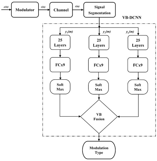
Figure 1.
Proposed System Model for Voting-Based DCNN.
The input span of the DCNN is normally fixed, and the length of the signal to be classified may be much larger than this length. Aiming to use signal complete information for better accuracy, the input signal is divided into many segments of length L. Every segment is fed to the DCNN, and the voting-based fusion method gains the result. The received signal of length N is segmented by sliding at the P interval and then choosing every signal segment of span L. The segmentation of the signal is described in Equation (2) as follows:
where m = 0, 1, 2, …, (L − 1) and i = 1, 2, …, . The signal is segmented with a length of .
4. Voting-Based DCNN
4.1. Deep Convolutional Neural Network
The deep convolutional neural network is designed for the classification of modulation formats as shown in Figure 2. The DCNN architecture comprises 28 layers, including an input layer, convolutional layer, ReLU layer, Max pool layer, fully connected layer (FCL), softmax layer, and classification layer. The served as input to the DCNN layers, the CNN represents the convolution kernel, and the following number indicates the number of convolution kernels. The abbreviation “ReLU” stands for rectification linear activation. The softmax denotes the maximum number of neurons; the category is the final output, and the one-hot encoding is used for the category label. There is also a batch normalization layer between the convolutional layer and the nonlinear activation layer; for clarity, the layer is not depicted in Figure 2.
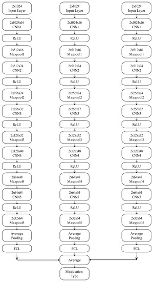
Figure 2.
Proposed Deep Convolutional Neural Network Layers [25].
4.2. Voting-Based Fusion
In this paper, voting-based fusion has been utilized to improve the classification accuracy of the VB-DCNN. Segmented signals are fed to the deep convolution neural network; the outputs are obtained at the classification layer. The modulation type of signal is obtained by fusing the classification results, i.e., voting-based fusion. VB fusion is the general fusion method employing the majority wins rule. The class with the most votes is considered the classification output [32]. The classification results are denoted [1, 2, 3, …, M]. From the , the
The number of times the classification is k-th modulation is presented as follows:
The final decision on voting-based fusion is the maximum argument of the , i.e.,
The proposed algorithm for the VB-DCNN classifier is given in Algorithm 1.
| Algorithm 1: VB-DCNN classifier. |
 |
4.3. Computational Complexity of VB-DCNN
The computational complexity of the proposed algorithm is demonstrated in Table 1. The size of the input signal is , it is passed through the CNN1 of size as shown in Figure 2, and the number of parameters is . Accordingly, the output will be and the total number of parameters calculated are , i.e., 32. The number of parameters in the Max pool layer is 32 as well. Similarly, the number of parameters at each layer is calculated using the same procedure.

Table 1.
Computational Complexity of Proposed Algorithm.
5. Simulation Results
The M-PSK, M-FSK, and M-QAM signals have been considered for classification throughout the simulations. The dataset is generated for different modulations and consists of 10,000 samples per frame. A trained model is based on 80% of the dataset, and a test and a validated model is based on 10% of the dataset. The performance of the proposed VB-DCNN is also evaluated on a fading channel in the presence of AWGN. The figure of merit (FoM) is the percentage classification accuracy (PCA). All the simulations are on the Matlab software 2020(a) version. The specification of the PC is 16 GB of RAM with core i-7, 2.60 GHz, a 10th-generation processor, and built-in GPU hardware. The simulation parameters are shown in Table 2.
Table 2.
Simulation Parameters.
The following are the three cases used to evaluate the performance of the proposed classifier:
- Case-I: M-PSK and MFSK signals;
- Case-II: M-QAM signals;
- Case-III: nine modulated signals.
The received signal may be a PSK or FSK signal, a QAM signal, or PSK and QAM signals. A separate model is trained for each case to validate the efficiency of the proposed algorithm.
5.1. Case-I: BPSK, QPSK, 8 PSK, 256 PSK, GFSK, CPFSK
The training of the VB-DCNN classifier for case-I is shown in Figure 3. The M-PSK and M-FSK signals are trained with 3750 and 750 iterations per epoch. The training accuracy is 100% with less than 100 iterations. From Figure 3, it is evident that the classifier is trained efficiently at 5 dB of SNR with a simulation time of 1 min and 49 s.
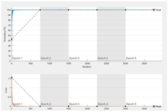
Figure 3.
VB-DCNN Training for Case-I.
The testing accuracy for case-I is 100% at 5 dB of SNR, which is taken for a single simulation. All the selected modulations are 100% classified, and the quantitative analysis in the form of a confusion matrix is shown in Figure 4.
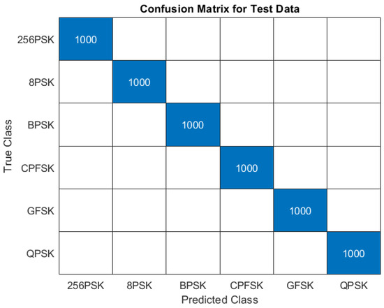
Figure 4.
Confusion Matrix for Case-I at SNR = 5 dB.
5.2. Case-II: 4 QAM, 8 QAM, 16 QAM, 256 QAM
The training and testing of the proposed VB-DCNN are evaluated for the QAM modulated signals, i.e., 4 QAM, 8 QAM, 16 QAM, and 256 QAM. The validation accuracy for case-II is 99.58% at 10 dB of SNR. The training and loss curves are shown in Figure 5, which shows the VB-DCNN is trained perfectly for the M-QAM signals. The training time is 1 min and 13 s, with 2500 and 500 iterations per epoch. In Figure 5, the black dashed line shows the validation curve, the blue dotted line shows the training curve, and the blue line shows the smoothed training curve.
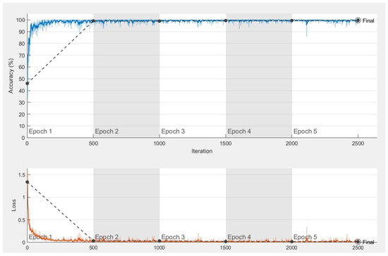
Figure 5.
VB-DCNN Training for Case-II.
The testing accuracy for case-II on an AWGN channel with an SNR of 10 dB is 99.47%. The classification accuracy for 16 QAM and 256 QAM is 99.7% and 98.2%, respectively. The classification accuracy for 4 QAM and 8 QAM is 100%. The quantitative analysis of the proposed VB-DCNN is shown in Figure 6. Since QAM modulates amplitude and phase, it is spectrally efficient, which is why QAM signals are hard to classify compared to PSK signals.
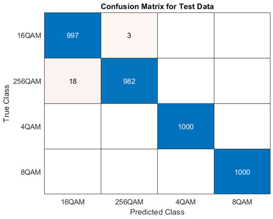
Figure 6.
Confusion Matrix for Case-II at SNR = 10 dB.
5.3. Case-III: Nine Modulated Signals
The joint classification of nine modulated signals, i.e., GFSK, CPFSK, BPSK, 8 PSK, 256 PSK, 4 QAM, 8 QAM, 16 QAM, and 256 QAM, is demonstrated in case-III. The validation accuracy is approximately 99.80% at an SNR of 10 dB, as shown in Figure 7. Figure 7 shows the training accuracy and loss curves. The maximum number of iterations to train the VB-DCNN for classifying 9 modulations is 5625, with 1125 iterations per epoch. The simulation time is 2 min and 45 s.
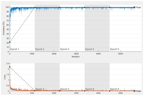
Figure 7.
VB-DCNN Training for Case-III.
The test accuracy of the proposed VB-DCNN classifier is exactly 99.68% at 10 dB of SNR. The VB-DCNN classifier accurately classifies the GFSK, CPFSK, 8 QAM, BPSK, 8 PSK, 4 QAM, and 256 PSK. For the 16 QAM, the classifier correctly classified 976 times and it misclassified 24 times. For the 256 QAM classification, the accuracy is 99.6% and 97.6% for the 16 QAM signal. The confusion matrix of the VB-DCNN is shown in Figure 8.
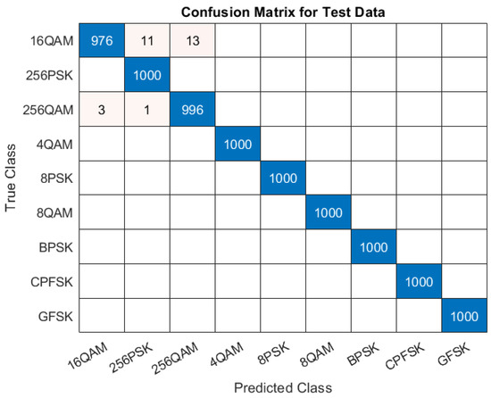
Figure 8.
Confusion Matrix for Case-III at SNR = 10 dB.
5.4. Performance Evaluation with Different Layers
The performance of the VB-DCNN for different numbers of layers is shown in Figure 9 at an SNR of 10 dB. As evident from Figure 9, the classification accuracy increases as the number of layers increases in the architecture. The classification accuracy for 28, 20, and 12 layers is 99.6%, 97.3%, and 90.2%, respectively.
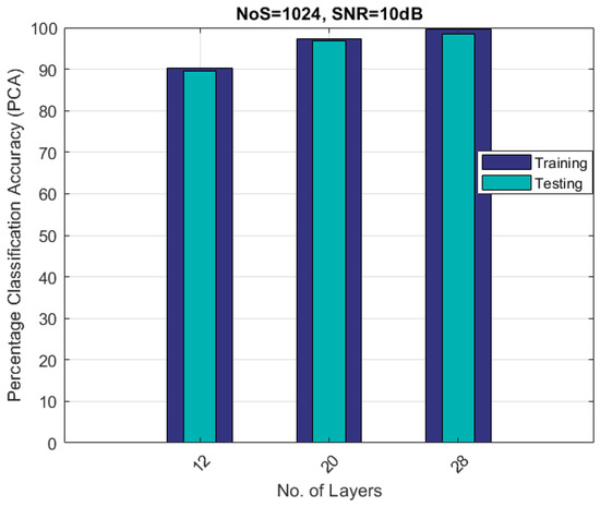
Figure 9.
PCA vs. No. of Layers.
5.5. VB-DCNN Performance Evaluation on Fading Channels
The performance of the VB-DCNN for nine different modulated signals is evaluated on AWGN, Rician, and Rayleigh fading channels. The training of the VB-DCNN on the AWGN, Rayleigh, and Rician channel models is shown in Figure 10 at SNRs of 5 and 10 dB. The training accuracy at 10 dB of SNR of the AWGN, Rayleigh, and Rician channels is 99%, 76%, and 80%, respectively. Figure 11 shows that the training accuracy on higher SNRs is much better than the lower SNRs. The testing accuracy of the proposed VB-DCNN on the fading channels is also shown in Figure 10 with quantitative analysis.
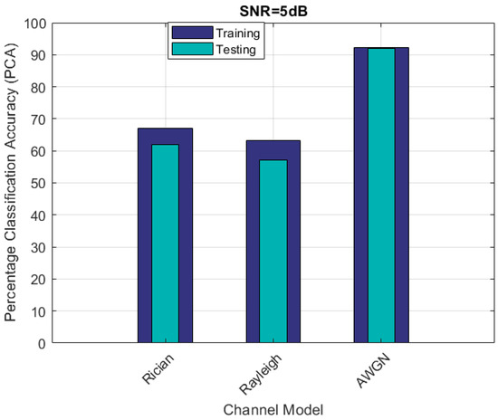
Figure 10.
VB-DCNN Performance Analysis on Fading Channels (SNR = 5 dB).
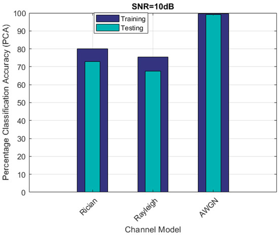
Figure 11.
VB-DCNN Performance Analysis on Fading Channels (SNR = 10 dB).
The classification accuracy for case-I is exactly 100%. This is primarily because there are six modulation classes, and the SNR considered is 5 dB. For case-II, however, the number of modulations considered is four, while the SNR is 10 dB. As a result, we are obtaining good classification accuracy for specific scenarios. Figure 12 illustrates that classification accuracy is low, and almost all modulations are unclassified; this is due to the dominance of noise over the entire signal, which contributes to poor classification accuracy. Due to the deep neural network design and, in particular, the fusion of the features, classification accuracy is also very high.
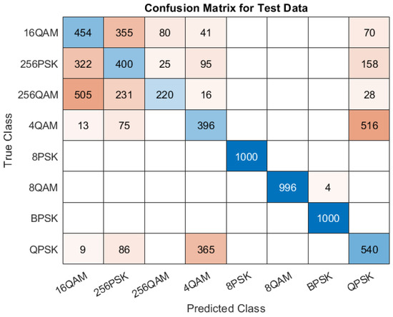
Figure 12.
Classification Accuracy at 0 dB.
5.6. Relationship Training and Testing Accuracy
The training accuracy of case-I, i.e., BPSK, QPSK, 8 PSK, 256 PSK, GFSK, and CPFSK, is shown in Figure 3, and the testing accuracy for case-I is shown in the form of a confusion matrix in Figure 4.
The training accuracy of case-II, i.e., 4 QAM, 8 QAM, 16 QAM, 256 QAM, is shown in Figure 5, and the testing accuracy for case-II is shown in the form of a confusion matrix in Figure 6.
The training accuracy of case-III is shown in Figure 7, and the testing accuracy for case-III is shown as a confusion matrix in Figure 8.
The relationship between testing and training accuracy for all the proposed cases is shown in Table 3. As clear from Table 3, there is a close relationship between the training and testing accuracy, suggesting that the proposed model is not over-fitted or under-fitted.
Table 3.
Training and Testing Accuracy.
5.7. Comparative Analysis of VB-DCNN
The classification accuracy of the proposed VB-DCNN with the state-of-the-art techniques is shown in Table 4. The number of samples is 1024, with an SNR of 0 dB and all the results in % classification accuracy. From Table 4, it is clear that the proposed classifier performs much better with the existing techniques, and in many cases, the classification accuracy approaches 100%.
Table 4.
Comparison of Proposed VB-DCNN Classifier with State-of-the-Art Existing Techniques.
As shown in Table 4, in [33], the authors present modulation classification based on CNN in the presence of interfering signals. The authors used ten different modulations for classification from the dataset of RadioML2016. The classification accuracy is presented in two scenarios: 5-class and 10-class problems. The model in [33] gives 70.9% accuracy while our proposed classifier gives a better accuracy of 100% at the same SNR, i.e., 0 dB.
In [34], the authors used the deep convolutional neural network to classify M-PSk and M-QAM modulation forms. The authors used a multi-stream comprehensive network structure to extract richer features. The authors classified the modulation formats at 8 dB of SNR and did not consider the higher, higher-order QAMs and PSKs. Convolution neural networks (CNNs) and gate rate units (GRUs) are used in a hybrid parallel structure to extract, respectively, spatial and temporal data [35]. The accuracy of [35] for the GFSK is not good at 0 dB of SNR, while for BPSK and CPFSK, the classifier accuracy is 100%. In [36], the authors use the cuckoo search algorithm to optimize the classification accuracy of the GFN-based modulation classifier. The authors employed various modulation techniques, but the classification accuracy is around 96% at 0 dB of SNR.
While comparing with other references, the classification accuracy of [34,35,36] is 98%, 100%, and 96.52%, respectively, for the BPSK modulation case scenario. The classification accuracy for the higher-order modulations, i.e., 256 PSK and 256 QAM, is above 80%, which is quite good at lower SNRs, i.e., 0 dB. To the best of our knowledge, there is no such scheme that classifies the higher-order PSK and QAM signals. The study [36] only considers the BPSK, 8 PSK, QAM, and 8 QAM signals for the classification. From Table 4, it is found that the proposed classifier for the single run gives 100% classification accuracy.
Simulations indicate that the proposed VB-DCNN performs better, but some limitations exist. The VB-DCNN requires large amounts of high-quality training data to achieve higher accuracy. Initially, training requires a careful selection of the parameters and a significant amount of complexity compared to the single-CNN architecture. However, the model is trained once, so the complexity can be a trade-off with the performance. Implementing the training with fewer resources may negatively affect performance.
6. Conclusions
This research work investigates the problem of higher-order modulation classification using a voting-based deep convolutional neural network. Raw signals are fed into the VB-DCNN classifier, passing the signal through different independent CNN architectures. The inputs from various layers are finally computed based on the majority of the votes. This results in better classification and efficient utilization of the entire signal spectrum. For the evaluation of the suggested classifier, different layers have been suggested, and it is found that increasing layers will give higher classification accuracy and vice versa. In addition, the proposed classification algorithm is tested on various fading channels with different SNRs. A performance comparison is conducted between the VB-DCNN classifier and current state-of-the-art techniques, and in a specific scenario, the accuracy of the classifier is close to 100%. The classification accuracy may be further improved by employing different window functions in the DCNN and developing CNNs that are robust to noise and interference in the future. The feature focus might be developing CNN-based classifiers that can operate effectively in resource-constrained environments, potentially using pruning or quantization compression techniques.
Author Contributions
Conceptualization, M.T., S.A.G., M.S. and R.M.M.; methodology, M.T., S.A.G., M.S. and A.R.; software, M.T., S.A.G., M.S. and A.R.; validation, S.A.G., M.S., A.R., M.A. and G.K.; formal analysis, M.T., S.A.G., M.S., A.R., R.M.M. and G.K.; investigation, M.T., S.A.G., A.R., M.A. and G.K.; resources, S.A.G., M.S., A.R., M.A. and G.K.; data curation, M.T., S.A.G., M.S. and A.R.; writing—original draft preparation, M.T., S.A.G., M.S., A.R., M.A., R.M.M. and G.K.; writing—review and editing, S.A.G., M.S., A.R., M.A. and G.K.; visualization, S.A.G., M.S., M.A., R.M.M. and G.K.; supervision, S.A.G. All authors have read and agreed to the published version of the manuscript.
Funding
This research received no external funding.
Institutional Review Board Statement
Not applicable.
Informed Consent Statement
Not applicable.
Data Availability Statement
Not applicable.
Conflicts of Interest
The authors declare no conflict of interest.
Notation
| (n) | Fading Coefficients |
| Length of Segmented Signal | |
| i-th Classification Class | |
| Voting-based Fusion | |
| L | length of the signal |
References
- Zhu, Z.; Nandi, A.K. Automatic Modulation Classification: Principles, Algorithms and Applications; John Wiley & Sons: Hoboken, NJ, USA, 2015. [Google Scholar]
- Mahmood, A.; Ahmed, A.; Naeem, M.; Amirzada, M.R.; Al-Dweik, A. Weighted utility aware computational overhead minimization of wireless power mobile edge cloud. Comput. Commun. 2022, 190, 178–189. [Google Scholar] [CrossRef]
- Sarfraz, M.; Alam, S.; Ghauri, S.A.; Mahmood, A.; Akram, M.N.; Rehman, M.; Sohail, M.F.; Kebedew, T.M. Random Graph-Based M-QAM Classification for MIMO Systems. Wirel. Commun. Mob. Comput. 2022, 2022, 9419764. [Google Scholar] [CrossRef]
- Wang, T.; Wen, C.K.; Jin, S.; Li, G.Y. Deep learning-based CSI feedback approach for time-varying massive MIMO channels. IEEE Wirel. Commun. Lett. 2018, 8, 416–419. [Google Scholar] [CrossRef]
- Wang, F.; Huang, S.; Wang, H.; Yang, C. Automatic modulation classification exploiting hybrid machine learning network. Math. Probl. Eng. 2018, 2018, 6152010. [Google Scholar] [CrossRef]
- Khan, W.U.; Lagunas, E.; Mahmood, A.; Chatzinotas, S.; Ottersten, B. When RIS meets geo satellite communications: A new optimization framework in 6G. arXiv 2022, arXiv:2202.00497. [Google Scholar]
- Ullah Khan, W.; Lagunas, E.; Mahmood, A.; Chatzinotas, S.; Ottersten, B. Integration of Backscatter Communication with Multi-cell NOMA: A Spectral Efficiency Optimization under Imperfect SIC. arXiv 2021, arXiv:2109.11509. [Google Scholar]
- Akeela, R.; Dezfouli, B. Software-defined Radios: Architecture, state-of-the-art, and challenges. Comput. Commun. 2018, 128, 106–125. [Google Scholar] [CrossRef]
- Bany Muhammad, N.; Ghauri, S.; Sarfraz, M.; Munir, S. Genetic algorithm assisted support vector machine for M-QAM classification. Math. Model. Eng. Probl. 2020, 7, 441–449. [Google Scholar]
- Wu, P.; Sun, B.; Su, S.; Wei, J.; Zhao, J.; Wen, X. Automatic modulation classification based on deep learning for software-defined radio. Math. Probl. Eng. 2020, 2020, 2678310. [Google Scholar] [CrossRef]
- Abu-Romoh, M.; Aboutaleb, A.; Rezki, Z. Automatic modulation classification using moments and likelihood maximization. IEEE Commun. Lett. 2018, 22, 938–941. [Google Scholar] [CrossRef]
- Aksoy, G.; Karabatak, M. Performance Comparison of New Fast Weighted Naïve Bayes Classifier with Other Bayes Classifiers. In Proceedings of the 2019 7th International Symposium on Digital Forensics and Security (ISDFS), Barcelos, Portugal, 10–12 June 2019; IEEE: Piscataway, NJ, USA, 2019; pp. 1–5. [Google Scholar]
- O’Shea, T.J.; Roy, T.; Clancy, T.C. Over-the-air deep learning based radio signal classification. IEEE J. Sel. Top. Signal Process. 2018, 12, 168–179. [Google Scholar] [CrossRef]
- Rajendran, S.; Meert, W.; Giustiniano, D.; Lenders, V.; Pollin, S. Deep learning models for wireless signal classification with distributed low-cost spectrum sensors. IEEE Trans. Cogn. Commun. Netw. 2018, 4, 433–445. [Google Scholar] [CrossRef]
- Ren, Y.; Jiang, W.; Liu, Y. Complex-valued Parallel Convolutional Recurrent Neural Networks for Automatic Modulation Classification. In Proceedings of the 2022 IEEE 25th International Conference on Computer Supported Cooperative Work in Design (CSCWD), Hangzhou, China, 4–6 May 2022; IEEE: Piscataway, NJ, USA, 2022; pp. 804–809. [Google Scholar]
- Chen, K.; Zhang, J.; Chen, S.; Zhang, S.; Zhao, H. Automatic modulation classification of radar signals utilizing X-net. Digit. Signal Process. 2022, 123, 103396. [Google Scholar] [CrossRef]
- Fu, X.; Gui, G.; Wang, Y.; Gacanin, H.; Adachi, F. Automatic Modulation Classification Based on Decentralized Learning and Ensemble Learning. IEEE Trans. Veh. Technol. 2022, 71, 7942–7946. [Google Scholar] [CrossRef]
- Huang, S.; Yao, Y.; Wei, Z.; Feng, Z.; Zhang, P. Automatic modulation classification of overlapped sources using multiple cumulants. IEEE Trans. Veh. Technol. 2016, 66, 6089–6101. [Google Scholar] [CrossRef]
- Aslam, M.W.; Zhu, Z.; Nandi, A.K. Automatic modulation classification using combination of genetic programming and KNN. IEEE Trans. Wirel. Commun. 2012, 11, 2742–2750. [Google Scholar]
- Ramjee, S.; Ju, S.; Yang, D.; Liu, X.; Gamal, A.E.; Eldar, Y.C. Fast deep learning for automatic modulation classification. arXiv 2019, arXiv:1901.05850. [Google Scholar]
- Meng, F.; Chen, P.; Wu, L.; Wang, X. Automatic modulation classification: A deep learning enabled approach. IEEE Trans. Veh. Technol. 2018, 67, 10760–10772. [Google Scholar] [CrossRef]
- Ke, Z.; Vikalo, H. Real-time radio technology and modulation classification via an LSTM auto-encoder. IEEE Trans. Wirel. Commun. 2021, 21, 370–382. [Google Scholar] [CrossRef]
- Liu, X.; Yang, D.; El Gamal, A. Deep neural network architectures for modulation classification. In Proceedings of the 2017 51st Asilomar Conference on Signals, Systems, and Computers, Pacific Grove, CA, USA, 29 October–1 November 2017; IEEE: Piscataway, NJ, USA, 2017; pp. 915–919. [Google Scholar]
- West, N.E.; O’Shea, T. Deep architectures for modulation recognition. In Proceedings of the 2017 IEEE International Symposium on Dynamic Spectrum Access Networks (DySPAN), Baltimore, MD, USA, 6–9 March 2017; IEEE: Piscataway, NJ, USA, 2017; pp. 1–6. [Google Scholar]
- Szegedy, C.; Liu, W.; Jia, Y.; Sermanet, P.; Reed, S.; Anguelov, D.; Erhan, D.; Vanhoucke, V.; Rabinovich, A. Going deeper with convolutions. In Proceedings of the IEEE Conference on Computer Vision and Pattern Recognition, Boston, MA, USA, 7–12 June 2015; pp. 1–9. [Google Scholar]
- Wang, N.; Liu, Y.; Ma, L.; Yang, Y.; Wang, H. Automatic Modulation Classification Based on CNN and Multiple Kernel Maximum Mean Discrepancy. Electronics 2022, 12, 66. [Google Scholar] [CrossRef]
- Elsagheer, M.M.; Ramzy, S.M. A hybrid model for automatic modulation classification based on residual neural networks and long short term memory. Alex. Eng. J. 2023, 67, 117–128. [Google Scholar] [CrossRef]
- Essai, M.H.; Atallah, H.A. Automatic Modulation Classification: Convolutional Deep Learning Neural Networks Approaches. SVU-Int. J. Eng. Sci. Appl. 2023, 4, 48–54. [Google Scholar]
- Xu, J.; Lin, Z. Modulation and Classification of Mixed Signals Based on Deep Learning. arXiv 2022, arXiv:2205.09916. [Google Scholar]
- Indira, N.D.; Rao, M.V.G. Deep Learning CNN-Based Hybrid Extreme Learning Machine with Bagging Classifier for Automatic Modulation Classification. Int. J. Intell. Syst. Appl. Eng. 2022, 10, 134–141. [Google Scholar]
- Ma, R.; Wu, D.; Hu, T.; Yi, D.; Zhang, Y.; Chen, J. Automatic Modulation Classification Based on One-Dimensional Convolution Feature Fusion Network. In Proceedings of the 2021 International Conference on Wireless Communications, Networking and Applications, Hangzhou, China, 13–15 August 2021; Springer: Berlin/Heidelberg, Germany, 2022; pp. 888–899. [Google Scholar]
- Zheng, S.; Qi, P.; Chen, S.; Yang, X. Fusion methods for CNN-based automatic modulation classification. IEEE Access 2019, 7, 66496–66504. [Google Scholar] [CrossRef]
- Triantaris, P.; Tsimbalo, E.; Chin, W.H.; Gündüz, D. Automatic modulation classification in the presence of interference. In Proceedings of the 2019 European Conference on Networks and Communications (EuCNC), Valencia, Spain, 18–21 June 2019; IEEE: Piscataway, NJ, USA, 2019; pp. 549–553. [Google Scholar]
- Zhang, H.; Wang, Y.; Xu, L.; Gulliver, T.A.; Cao, C. Automatic modulation classification using a deep multi-stream neural network. IEEE Access 2020, 8, 43888–43897. [Google Scholar] [CrossRef]
- Zhang, R.; Yin, Z.; Wu, Z.; Zhou, S. A novel automatic modulation classification method using attention mechanism and hybrid parallel neural network. Appl. Sci. 2021, 11, 1327. [Google Scholar] [CrossRef]
- Shah, S.I.H.; Coronato, A.; Ghauri, S.A.; Alam, S.; Sarfraz, M. CSA-Assisted Gabor Features for Automatic Modulation Classification. Circuits Syst. Signal Process. 2022, 41, 1660–1682. [Google Scholar] [CrossRef]
Disclaimer/Publisher’s Note: The statements, opinions and data contained in all publications are solely those of the individual author(s) and contributor(s) and not of MDPI and/or the editor(s). MDPI and/or the editor(s) disclaim responsibility for any injury to people or property resulting from any ideas, methods, instructions or products referred to in the content. |
© 2023 by the authors. Licensee MDPI, Basel, Switzerland. This article is an open access article distributed under the terms and conditions of the Creative Commons Attribution (CC BY) license (https://creativecommons.org/licenses/by/4.0/).