Study of Parameter Configuration on an Embedded System Used for Acoustic Leak Localization in Metallic Pipelines

Abstract

The subject of pipeline monitoring for a timely response in the case of leakage has raised intense interest and numerous leak localization methods have been presented in the literature. However, most approaches focus more on the performance of the methods themselves and not on their implementation on a typical embedded system and the way that the main system parameters affect its operation. The present paper aims to contribute to this field. Specifically, an acoustic leak localization method, developed in our previous research, is implemented in C++ on the Raspberry Pi 4B platform. The main system parameters are defined and certain trade-offs between them are examined. These trade-offs concern three basic metrics: the leak localization accuracy, the execution time of the algorithm, and the memory consumption, which rely on the values of the system parameters. Based on the targeted application, the importance of each of the aforementioned metrics can vary. For this reason, an evaluation function, equipped with user-defined weighting coefficients corresponding to the three metrics, is constructed in this paper. With the help of this function, a given parameter combination can be evaluated and the decision about its utilization in a certain application can be made.

1. Introduction

Pipeline networks are widely used in several different fields. They provide a safe and practical way to transport fluid products of any kind and they are encountered in many applications. However, a number of factors can affect the state of the pipelines and cause damage, which leads to the occurrence of leaks. Some typical examples of problems associated with leakages are the existence of defective valves or other faulty equipment, badly attached measuring instruments, corrosion of the pipe material, excavation accidents, or even intentional puncturing of the pipelines by third parties in an attempt to steal the carried product.

Pipeline leaks have serious consequences since they result in product loss (with an obvious financial impact), environmental pollution, disturbance of the surrounding fauna and even hazardous accidents. For this reason, extensive research has been conducted over the years, concerning the development of effective leak detection and localization methods [1,2,3,4]. These methods can rely on several physical phenomena from different areas, like optics [5,6,7,8,9], thermodynamics [10,11,12,13,14], acoustics [15,16,17,18,19,20,21,22,23,24,25,26], etc.

In the field of acoustics, that our research focuses on, numerous techniques have been reported in the literature. Na et al. [17] presented an adaptive leak localization method based on the Generalized Cross-Correlation (GCC) algorithm, which is needed for the estimation of the Time-Difference-Of-Arrival (TDOA) between the acoustic leak signals acquired by the installed sensors. However, as the authors stated, leak signals are usually corrupted by external noise, which results in a less accurate calculation of the leak position. In order to improve the localization accuracy, the authors combine the GCC algorithm with a Back-Propagation Neural Network (BPNN).

Li et al. [19] proposed an acoustic leak localization method, which relies on the utilization of the Cross-Time-Frequency Spectrum (CTFS) of the leak signals for the estimation of the leak position. Specifically, the coordinates of the peak of the CTFS are a time value and a frequency value. The time value is considered as the TDOA between the leak signals and the frequency corresponds to a certain value for the acoustic velocity, through the dispersion curve of the dominant wave mode. Then, the TDOA and velocity values are used for the calculation of the leak position. As the authors explained, this approach provides better localization accuracy than the traditional cross-correlation technique.

On the other hand, Ting et al. [23] proposed an acoustic method that presents improved localization results in comparison to other conventional methods. They used the Dual-Tree Complex Wavelet Transform (DTCWT) in order to suppress the ambient noise from the leak signals before applying the cross-correlation algorithm to them, thus enhancing the accuracy of the TDOA estimation. Furthermore, Quy et al. [24] presented a leak localization method that detects Acoustic Emission (AE) bursts in the leak signals via adaptive thresholds and uses them to identify the position of the leak point by combining a wave propagation model with signal processing. This way they achieved lower localization error than other reported methods.

As can be observed from the discussion above, in the procedure of designing a leak localization method, researchers mainly focus on certain factors impacting the effectiveness of the method in the estimation of the leak position and try to provide solutions that increase the localization accuracy. However, another important aspect that needs to be considered is the implementation of the developed method on the available hardware. When a real-time leak monitoring system is placed permanently on a pipeline, a very common approach is to build it by installing several autonomous nodes, which are able to communicate with each other, conduct measurements and process the acquired leak data. These nodes are typical examples of embedded systems. Hence, apart from the accuracy in the calculation of the leak position, a study about the performance of the designed method on the employed embedded system should also be conducted.

Despite its importance, this kind of study is usually not included in the relevant literature. So, the goal of the present article is to contribute to this area. For this reason, an acoustic leak localization method is implemented on a typical embedded system. This method, which was designed and presented in our previous work [27], relies on the installation of two accelerometer sensors at both ends of the pipeline under protection and on the utilization of a certain localization algorithm that combines the cross-correlation technique with temporal and spectral segmentation of the leak signals. In the present paper, this method is implemented in C++ on the Raspberry Pi 4B [28] hardware platform. Then, the main parameters of this embedded system are taken into consideration and certain trade-offs are examined. Specifically, a study is conducted about the impact that the values of the system parameters have on three different metrics: (a) the localization error, (b) the execution time of the method on the employed hardware platform, and (c) the memory consumption. Another important metric could be the energy consumed by the embedded system. However, the energy is directly associated with the execution time (i.e., larger execution time leads to higher energy consumption) and, therefore, it is not considered an independent metric. An evaluation function is constructed, based on which a success rate is attributed to a given parameter combination, thus providing an idea about its effectiveness in a certain application. Moreover, experimental results about the aforementioned trade-offs are presented, with the help of real leak measurements conducted on a laboratory pipeline setup, and certain conclusions are drawn.

2. Materials and Methods

As mentioned earlier, for the study conducted in this paper, an acoustic leak localization method was implemented on the employed embedded system. Since this method was described thoroughly in [27], here we will just review its main steps, because we are going to need some of its basic concepts when we define the system parameters. This method uses the recorded acoustic leak signals from two accelerometer sensors mounted externally on the pipe surface at a distance L between them, as shown in Figure 1. The basic steps of the method are the following:

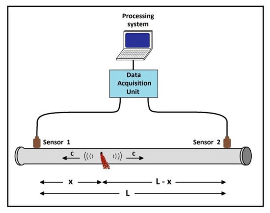
Figure 1. Sensor placement for acoustic leak localization.

• Step 1: The acoustic signals acquired by the two sensors are segmented into a number of N_F equally sized spectral bands, via FIR filters.
• Step 2: The signal in each spectral band is fragmented into N_T temporal portions.
• Step 3: Each portion of each spectral band from Sensor 1 is cross-correlated with its corresponding portion from Sensor 2. At the end of this step, N_T values for the time lag Δn (expressed in samples) between the signals from the two sensors are produced in each spectral band. The time lag Δn (Δn = F_S∙Δt), along with the value of the propagation velocity of the vibroacoustic waves, are crucial for the successful estimation of the leak position.
• Step 4: The Δn values considered as outliers are rejected and then from the ones that remain, the dominant Δn value (i.e., the most frequently appeared) in each spectral band is selected. This can be expressed mathematically as follows:

  $$\Delta n_i=\underset{j=1}{\overset{N_T}{MF}}\left[\arg \max \left(R_{ij}\right)\right]$$

  (1)

  where R_ij is the cross-correlation function between the corresponding portions (mentioned in Step 3) of the signals, Δn_i is the dominant Δn value of the ith band and MF is defined as an operator that extracts the dominant Δn value of each spectral band, after rejecting the outliers. Then, an estimation (x_i) of the leak position is derived for each band, based on the following relationship:

  $$x_i=\frac{1}{2}\left(L+c_i\frac{\Delta n_i}{F_S}\right)=\frac{1}{2F_S}\left\{F_{S}L+c_i\cdot \underset{j=1}{\overset{N_T}{MF}}\left[\arg \max \left(R_{ij}\right)\right]\right\}$$

  (2)

  where F_S is the sampling frequency and c_i is the propagation velocity of the acoustic waves for the ith band.
• Step 5: The final value of the leak position (x) is calculated as a weighted mean of the position estimates (i.e., the x_i’s) from all the spectral bands, by using the following equation:

  $$x=\frac{{\displaystyle \sum _{i=1}^{N_F}{x}_i{w}_i}}{{\displaystyle \sum _{i=1}^{N_F}{w}_i}}\Rightarrow x=\frac{{\displaystyle \sum _{i=1}^{N_F}\left\{F_{S}L+c_i\cdot \underset{j=1}{\overset{N_T}{MF}}\left[\arg \max \left(R_{ij}\right)\right]\right\}{w}_i}}{2F_S\cdot {\displaystyle \sum _{i=1}^{N_F}{w}_i}}$$

  (3)

  where w_i is the weighting coefficient of the ith spectral band. The weighting coefficients are derived in the preliminary stage of the localization method, as described in [27].

This method presents efficient leak localization results, compared to other relevant methods in the literature, with an average localization error of 4.3%.

The embedded system on which the leak localization method described above was implemented is the Raspberry Pi 4 (Model B) hardware platform shown in Figure 2. This platform contains a 64-bit quad-core ARM Cortex-A72 processor at 1.5 GHz, 4 GB RAM, a micro-SD card used both for data storing and for the operating system (i.e., Raspbian OS), as well as a number of different interfaces, like HDMI, Ethernet, USB connectors, a 40-pin GPIO (General Purpose Input/Output) header, etc. The localization method was implemented on this particular platform by using the C++ programming language.

Figure 2. Raspberry Pi 4 (Model B) hardware platform.

The main parameters of the employed embedded system that were taken into consideration in this study are the following:

• W_F: the width of the spectral bands (in Hz).
• W_T: the width of the temporal portions (in samples).
• Dur: the duration of the leak measurements (in samples).
• F_S: the sampling frequency (in Hz).
• Bits: the number of bits in the representation of the sample values.
• Taps: the number of taps of the designed FIR filters.

The values of the aforementioned parameters have an impact on the functionality of the system, since they affect the quality of the results (i.e., localization accuracy), as well as the system performance, which includes the execution time, the energy consumption, and the memory consumption. Due to the direct connection between the execution time and the energy consumption, as explained in the introduction, the following three independent metrics are selected for the present study: (a) the localization error, (b) the execution time, and (c) the memory consumption. Then, different combinations for the values of the system parameters are employed and certain trade-offs between them are examined.

In order to obtain some quantitative results about the studied trade-offs, an evaluation function is constructed. This function uses the three metrics as its independent variables and the value of the function serves as the success rate for the employed combination of the three metrics. However, since the values of the metrics are directly related to the selected configuration of the system parameters, the evaluation function can provide a rating for a given parameter configuration.

In the present study, we define the evaluation function (F_ev) as follows:

$$F_{ev}\left(E,T,M\right)=A_1\cdot e^{-\frac{E}{E_0}}+A_2\cdot e^{-\frac{T}{T_0}}+A_3\cdot e^{-\frac{M}{M_0}}$$

(4)

where E is the localization error; T is the execution time; M is the memory consumption; and E₀, T₀, and M₀ are constants. Moreover, the quantities A₁, A₂, and A₃ are constant coefficients, whose values are defined based on the targeted application. For example, if the leak localization accuracy is of major importance, the coefficient A₁ (for the localization error) will be greater than the other two. On the other hand, if we have an application where the quick response of the leak localization system is of the essence, then the coefficient A₂ (for the execution time) will have the largest value, and so on. The three coefficients A₁, A₂ and A₃ satisfy the following normalization gauge:

$${\displaystyle \sum _{i=1}^3{A}_i}=1$$

(5)

So that the evaluation function is bounded between the values 0 and 1. The value “F_ev = 1” corresponds to a perfect score (ideal case) and the value “F_ev = 0” to the exact opposite (worst case). When a certain parameter combination is selected, the values of the localization error, the execution time, and the memory consumption are carried out and then they are inserted into the evaluation function in order to calculate the score that will be assigned to this combination, based on Equation (4).

The evaluation function in the present study was designed to have an exponential form. The reason for this is that we want the evaluation to be somewhat stricter at the region of interest, which is the area where the score achieved for a given parameter combination is above a certain level defined by the user. Additionally, the values of the constants E₀, T₀, and M₀ can be configured properly in order to regulate the steepness of the evaluation function curve and, consequently, define the region of interest. In this study, these values are the following: E₀ = 50%, T₀ = 240 s, and M₀ = 8192 KB. When the localization error, the execution time, and the memory consumption reach the values of E₀, T₀, and M₀, respectively, the score achieved by the evaluation function drops to 1/e ≈ 0.37.

3. Results

The study of the system parameters in this article was conducted based on real leak measurements from a laboratory pipeline setup. This setup includes a 3 ½ inch steel pipeline containing water, with a total length of 90 m, which forms a closed circuit. An expansion tank is used for the regulation of the pressure inside the pipe. A circulator is employed in order to adjust the flow rate of the water at the desired value. Moreover, three valves with configurable orifice diameters are utilized for the emulation of leaks. The two accelerometer sensors were mounted on the pipe at a distance L = 66.83 m between them, as shown in Figure 3. In the same figure the positions of the leak points, with respect to the location of the first sensor, are presented as well. Additionally, it should be noted that recorded noise from the Hellenic Petroleum [29] refinery in Thessaloniki was added to the leak measurements in order to emulate the actual conditions in the field.

Figure 3. A section of the laboratory pipeline (on the left) and a schematic of its full topology along with the locations of the leak points (on the right).

In this paper, three different leak diameters were employed: 3 mm, 5 mm, and 7 mm. Initially, a 3 mm leak measurement is used in order to conduct a first examination of the system parameters. Specifically, the following values were assigned to the system parameters during this procedure:

• For W_T: 32,768 samples, 65,536 samples, 131,072 samples, and 262,144 samples.
• For W_F: 800 Hz and 1600 Hz.
• For Dur: 131,072 samples, 262,144 samples, and 524,288 samples.
• For F_S: 12.8 kHz and 25.6 kHz.
• For Bits: 10, 16, and 24.
• For Taps: 47 and 63.

By using the values mentioned above, a number of 144 parameter combinations were formed (this number is less than the total number of the possible combinations that would be obtained if we used all the different values for all parameters because some values cannot be combined with some others). From the derived combinations, the ones that provided the most efficient performance were selected for further examination, with the help of the evaluation function. The selected parameter combinations were applied on all three leak diameters and the obtained results are presented in Table 1, Table 2, Table 3, Table 4, Table 5, Table 6, Table 7, Table 8, Table 9 and Table 10. In these tables, the values of the system parameters are presented on the left side. In the middle, the location and diameter of each leak along with the execution time, the estimated leak position, and the localization error for each leak case can be observed and, on the right side, the average error, the average execution time, and the memory consumption for the given parameter combination are included.

Table 1. Parameter combination 1.

Parameter Values	Leak	Execution Time	Estimated Leak Position	Localization Error
WT = 65,536 Samp. WF = 800 Hz Bits = 24 FS = 25.6 kHz Dur = 262,144 Samp. Taps = 47	3 mm-B	16 s	19.29 m	1.6%	Average error: 3.1% Average execution time: 16 s Memory: 1.5 MB
	3 mm-C	16 s	21.56 m	0.5%
	5 mm-A	16 s	19.27 m	6.1%
	5 mm-B	16 s	18.30 m	0.1%
	5 mm-C	16 s	20.44 m	1.2%
	7 mm-A	16 s	16.26 m	1.6%
	7 mm-B	16 s	25.00 m	10.2%
	7 mm-C	16 s	23.54 m	3.5%

Table 2. Parameter combination 2.

Parameter Values	Leak	Execution Time	Estimated Leak Position	Localization Error
WT = 32,768 Samp. WF = 800 Hz Bits = 24 FS = 12.8 kHz Dur = 262,144 Samp. Taps = 63	3 mm-B	6 s	21.24 m	4.6%	Average error: 6.4% Execution time: 6 s Memory: 1.5 MB
	3 mm-C	6 s	17.21 m	6.0%
	5 mm-A	6 s	15.20 m	0.0%
	5 mm-B	6 s	23.17 m	7.4%
	5 mm-C	6 s	22.18 m	1.5%
	7 mm-A	6 s	19.63 m	6.6%
	7 mm-B	6 s	27.12 m	13.3%
	7 mm-C	6 s	29.05 m	11.7%

Table 3. Parameter combination 3.

Parameter Values	Leak	Execution Time	Estimated Leak Position	Localization Error
WT = 65,536 Samp. WF = 800 Hz Bits = 16 FS = 25.6 kHz Dur = 262,144 Samp. Taps = 47	3 mm-B	16 s	19.50 m	1.9%	Average error: 3.6% Execution time: 16 s Memory: 1 MB
	3 mm-C	16 s	20.56 m	1.0%
	5 mm-A	16 s	19.27 m	6.1%
	5 mm-B	16 s	18.30 m	0.1%
	5 mm-C	16 s	19.65 m	2.3%
	7 mm-A	16 s	16.26 m	1.6%
	7 mm-B	16 s	26.36 m	12.2%
	7 mm-C	16 s	23.54 m	3.5%

Table 4. Parameter combination 4.

Parameter Values	Leak	Execution Time	Estimated Leak Position	Localization Error
WT = 65,536 Samp. WF = 1600 Hz Bits = 10 FS = 25.6 kHz Dur = 524,288 Samp. Taps = 47	3 mm-B	16 s	17.09 m	1.7%	Average error: 5.8% Execution time: 16 s Memory: 1.25 MB
	3 mm-C	16 s	20.46 m	1.1%
	5 mm-A	16 s	22.06 m	10.3%
	5 mm-B	16 s	15.89 m	3.5%
	5 mm-C	16 s	21.09 m	0.2%
	7 mm-A	16 s	15.89 m	1.0%
	7 mm-B	16 s	28.24 m	15.0%
	7 mm-C	16 s	30.50 m	13.9%

Table 5. Parameter combination 5.

Parameter Values	Leak	Execution Time	Estimated Leak Position	Localization Error
WT = 131,072 Samp. WF = 800 Hz Bits = 24 FS = 25.6 kHz Dur = 524,288 Samp. Taps = 47	3 mm-B	57 s	16.39 m	2.7%	Average error: 2.5% Execution time: 57 s Memory: 3 MB
	3 mm-C	57 s	21.23 m	0.0%
	5 mm-A	57 s	16.41 m	1.8%
	5 mm-B	57 s	19.11 m	1.4%
	5 mm-C	57 s	22.88 m	2.5%
	7 mm-A	57 s	13.45 m	2.6%
	7 mm-B	57 s	22.88 m	7.0%
	7 mm-C	57 s	22.61 m	2.1%

Table 6. Parameter combination 6.

Parameter Values	Leak	Execution Time	Estimated Leak Position	Localization Error
WT = 131,072 Samp. WF = 800 Hz Bits = 24 FS = 25.6 kHz Dur = 262,144 Samp. Taps = 63	3 mm-B	29 s	15.49 m	4.1%	Average error: 4.6% Execution time: 29 s Memory: 1.5 MB
	3 mm-C	29 s	20.40 m	1.2%
	5 mm-A	29 s	21.37 m	9.2%
	5 mm-B	29 s	19.72 m	2.3%
	5 mm-C	29 s	22.34 m	1.7%
	7 mm-A	29 s	17.65 m	3.7%
	7 mm-B	29 s	24.98 m	10.1%
	7 mm-C	29 s	24.11 m	4.3%

Table 7. Parameter combination 7.

Parameter Values	Leak	Execution Time	Estimated Leak Position	Localization Error
WT = 65,536 Samp. WF = 800 Hz Bits = 16 FS = 12.8 kHz Dur = 262,144 Samp. Taps = 63	3 mm-B	8 s	18.83 m	0.9%	Average error: 1.9% Execution time: 8 s Memory: 1 MB
	3 mm-C	8 s	21.44 m	0.4%
	5 mm-A	8 s	17.00 m	2.7%
	5 mm-B	8 s	19.43 m	1.8%
	5 mm-C	8 s	20.99 m	0.3%
	7 mm-A	8 s	18.83 m	5.4%
	7 mm-B	8 s	17.33 m	1.3%
	7 mm-C	8 s	19.44 m	2.6%

Table 8. Parameter combination 8.

Parameter Values	Leak	Execution Time	Estimated Leak Position	Localization Error
WT = 131,072 Samp. WF = 800 Hz Bits = 10 FS = 25.6 kHz Dur = 262,144 Samp. Taps = 47	3 mm-B	28 s	21.62 m	5.1%	Average error: 4.0% Execution time: 28 s Memory: 640 KB
	3 mm-C	28 s	18.02 m	4.8%
	5 mm-A	28 s	15.49 m	0.4%
	5 mm-B	28 s	21.61 m	5.1%
	5 mm-C	28 s	20.97 m	0.4%
	7 mm-A	28 s	20.97 m	8.6%
	7 mm-B	28 s	22.19 m	6.0%
	7 mm-C	28 s	20.07 m	1.7%

Table 9. Parameter combination 9.

Parameter Values	Leak	Execution Time	Estimated Leak Position	Localization Error
WT = 65,536 Samp. WF = 800 Hz Bits = 10 FS = 12.8 kHz Dur = 262,144 Samp. Taps = 63	3 mm-B	8 s	19.46 m	1.9%	Average error: 2.9% Execution time: 8 s Memory: 640 KB
	3 mm-C	8 s	22.07 m	1.3%
	5 mm-A	8 s	19.46 m	6.4%
	5 mm-B	8 s	20.06 m	2.8%
	5 mm-C	8 s	20.53 m	1.0%
	7 mm-A	8 s	19.46 m	6.4%
	7 mm-B	8 s	17.00 m	1.8%
	7 mm-C	8 s	20.08 m	1.7%

Table 10. Parameter combination 10.

Parameter Values	Leak	Execution Time	Estimated Leak Position	Localization Error
WT = 262,144 Samp. WF = 800 Hz Bits = 24 FS = 25.6 kHz Dur = 262,144 Samp. Taps = 63	3 mm-B	31 s	12.37 m	8.7%	Average error: 4.7% Execution time: 31 s Memory: 1.5 MB
	3 mm-C	31 s	20.19 m	1.5%
	5 mm-A	31 s	20.74 m	8.3%
	5 mm-B	31 s	20.55 m	3.5%
	5 mm-C	31 s	20.67 m	0.8%
	7 mm-A	31 s	14.48 m	1.5%
	7 mm-B	31 s	25.01 m	10.2%
	7 mm-C	31 s	23.09 m	2.8%

In the column named “Leak”, the following nomenclature was adopted: each leak is named Xmm-Y, where X represents the diameter of the leak orifice (in mm) and Y corresponds to the employed leak point, according to Figure 3. So, for example, 5 mm-A is a 5 mm leak located at the point “Leak A” from Figure 3, 7 mm-B means a 7 mm leak at the point “Leak B”, etc. Additionally, it should be mentioned that the 3 mm-A leak was used in the leak localization method for the derivation of the weight coefficients and the velocity values of the different spectral bands of the acoustic signals. Due to this, the aforementioned leak always achieves perfect localization results (i.e., 0% error). So, in order for the evaluation of the parameter combinations to be fair, the 3 mm-A leak was omitted from Table 1, Table 2, Table 3, Table 4, Table 5, Table 6, Table 7, Table 8, Table 9 and Table 10.

At this point, the values of the average localization error, the execution time, and the memory consumption of each parameter combination in Table 1, Table 2, Table 3, Table 4, Table 5, Table 6, Table 7, Table 8, Table 9 and Table 10 can be inserted into the evaluation function in order to calculate the score for each combination. As explained in the previous section of the article, the values of the quantities A₁, A₂, and A₃ can be configured properly, according to the requirements of the targeted application. So, in the following tables, three different sets of values for the aforementioned quantities were formed and then the evaluation function was applied to each parameter combination. Specifically, in the first set (Table 11), we have A₁ = 0.6 and A₂ = A₃ = 0.2, thus giving more emphasis on localization accuracy. This could be the case when the monitored pipeline is located underground or in a remote place and, therefore, the accurate estimation of the leak position is very important. In the second set (Table 12), the quantity A₂ has a value of 0.6, while A₁ = A₃ = 0.2, so we focus on the execution time (and equivalently on the energy) of the localization algorithm. A parameter combination that provides low execution time would be very useful in certain applications such as in a pipeline system in a refinery, where a timely response to a leak event that can prove hazardous is of the essence. Finally, in the third set (Table 13), priority is given to memory consumption since the value of A₃ is equal to 0.6 and A₁ = A₂ = 0.2. Such a set could be required when the embedded system hosting the leak localization algorithm has limited memory capabilities.

Table 11. Evaluating the parameter combinations presented in Table 1, Table 2, Table 3, Table 4, Table 5, Table 6, Table 7, Table 8, Table 9 and Table 10 after setting A₁ = 0.6, A₂ = 0.2, and A₃ = 0.2 in the evaluation function.

Combination Name	Score	Combination Name	Score
Parameter combination 1	Fev = 0.92	Parameter combination 6	Fev = 0.89
Parameter combination 2	Fev = 0.89	Parameter combination 7	Fev = 0.95
Parameter combination 3	Fev = 0.92	Parameter combination 8	Fev = 0.92
Parameter combination 4	Fev = 0.89	Parameter combination 9	Fev = 0.94
Parameter combination 5	Fev = 0.87	Parameter combination 10	Fev = 0.89

Table 12. Evaluating the parameter combinations presented in Table 1, Table 2, Table 3, Table 4, Table 5, Table 6, Table 7, Table 8, Table 9 and Table 10 after setting A₁ = 0.2, A₂ = 0.6, and A₃ = 0.2 in the evaluation function.

Combination Name	Score	Combination Name	Score
Parameter combination 1	Fev = 0.92	Parameter combination 6	Fev = 0.88
Parameter combination 2	Fev = 0.93	Parameter combination 7	Fev = 0.95
Parameter combination 3	Fev = 0.92	Parameter combination 8	Fev = 0.90
Parameter combination 4	Fev = 0.91	Parameter combination 9	Fev = 0.95
Parameter combination 5	Fev = 0.80	Parameter combination 10	Fev = 0.88

Table 13. Evaluating the parameter combinations presented in Table 1, Table 2, Table 3, Table 4, Table 5, Table 6, Table 7, Table 8, Table 9 and Table 10 after setting A₁ = 0.2, A₂ = 0.2, and A₃ = 0.6 in the evaluation function.

Combination Name	Score	Combination Name	Score
Parameter combination 1	Fev = 0.87	Parameter combination 6	Fev = 0.86
Parameter combination 2	Fev = 0.87	Parameter combination 7	Fev = 0.92
Parameter combination 3	Fev = 0.90	Parameter combination 8	Fev = 0.93
Parameter combination 4	Fev = 0.88	Parameter combination 9	Fev = 0.94
Parameter combination 5	Fev = 0.76	Parameter combination 10	Fev = 0.86

As it can be observed by the score that the different parameter combinations achieve in Table 11, Table 12 and Table 13, some combinations are better at localizing the leak point accurately, providing low execution time or saving memory space, while others are effective in two or all three of the aforementioned tasks. For example, parameter combination 2 provides the best results in Table 12, where the emphasis is placed on the execution time. Parameter combination 5 achieves the highest score in Table 11, where the localization accuracy is prioritized, and the lowest one in Table 13, where the focus is on memory consumption. On the other hand, parameter combinations 7 and 9 achieve a high score in all situations. These two combinations differ only in the number of bits. As shown in Table 7 and Table 9, the execution time is the same for the two combinations, as expected, but there is a slight difference in the other two metrics. Specifically, parameter combination 7 (with 16 bits) provides better localization accuracy, while parameter combination 9 (with 10 bits) leads to less memory consumption. So, based on the requirements of the targeted application, the proper combination can be selected.

4. Discussion

In this paper, a study concerning the impact of the parameter configuration on the performance of an embedded system utilized for pipeline leak localization was presented. Initially, six different system parameters are defined: (i) the width of the temporal portions of the acoustic leak signals (derived from the segmentation of the signals in the time domain), (ii) the width of the spectral bands (obtained by the segmentation of the signals in the frequency domain), (iii) the duration of the leak measurements, (iv) the sampling frequency, (v) the number of bits used for the digital representation of the signal samples, and (vi) the number of taps of the employed FIR filters. Then, a large number of different combinations from these parameters were applied to leak measurements from a pipeline setup and certain trade-offs were examined. Specifically, these trade-offs concern the following three metrics: (a) the localization accuracy, (b) the execution time, and (c) the memory consumption. The energy consumption of the embedded system was also taken into account, but since it is directly connected to the execution time (varying similarly to the latter), it was not considered an independent metric and, therefore, not included in the calculations.

From the studied parameter combinations, the ones that provided the most efficient results were selected for further examination with the help of an evaluation function constructed in this paper. This function includes user-defined coefficients that allow the study to focus on certain metrics. The evaluation function was applied to the selected parameter combinations and corresponding results were presented. From these results, useful conclusions were drawn for the configuration of the system parameters in the targeted applications.

The present article is a novel contribution to the relevant literature since the majority of the published papers concerning the acoustic leak localization procedure emphasize only the development of effective methods and not their implementation on available embedded systems with certain capabilities and limitations. In future research, the study conducted in this paper could be extended to cover other types of pipelines (e.g., plastic, ceramic, etc.) and also different kinds of embedded systems.

References

- Korlapati, N.V.S.; Khan, F.; Noor, Q.; Mirza, S.; Vaddiraju, S. Review and analysis of pipeline leak detection methods. J. Pipeline Sci. Eng. 2022, 2, 100074. [Google Scholar] [CrossRef]
- Murvay, P.S.; Silea, I. A survey on gas leak detection and localization techniques. J. Loss Prev. Process Ind. 2012, 25, 966–973. [Google Scholar] [CrossRef]
- Boaz, L.; Kaijage, S.; Sinde, R. An Overview of Pipeline Leak Detection and Location Systems. In Proceedings of the 2nd Pan African International Conference on Science, Computing and Telecommunications, Arusha, Tanzania, 14–18 July 2014. [Google Scholar] [CrossRef]
- Behari, N.; Sheriff, M.Z.; Rahman, M.A.; Nounou, M.; Hassan, I.; Nounou, H. Chronic leak detection for single and multiphase flow: A critical review on onshore and offshore subsea and arctic conditions. J. Nat. Gas Sci. Eng. 2020, 81, 103460. [Google Scholar] [CrossRef]
- Kothandaraman, M.; Law, Z.; Ezra, M.A.G.; Pua, C.H. Adaptive Independent Component Analysis–Based Cross-Correlation Techniques along with Empirical Mode Decomposition for Water Pipeline Leakage Localization Utilizing Acousto-Optic Sensors. J. Pipeline Syst. Eng. Pract. 2020, 11, 04020027. [Google Scholar] [CrossRef]
- Ibrahim, K.; Tariq, S.; Bakhtawar, B.; Zayed, T. Application of fiber optics in water distribution networks for leak detection and localization: A mixed methodology-based review. H2Open J. 2021, 4, 244–261. [Google Scholar] [CrossRef]
- Law, Z.J.; Pua, C.H.; ShengLin, H.; Rahman, F.A. Application of Fiber Laser Dynamics in Leak Detection for Operating Water Pipeline. In Proceedings of the 12th International Conference on Sensing Technology (ICST), Limerick, Ireland, 4–6 December 2018. [Google Scholar] [CrossRef]
- Huang, Y.; Wang, Q.; Shi, L.; Yang, Q. Underwater gas pipeline leakage source localization by distributed fiber-optic sensing based on particle swarm optimization tuning of the support vector machine. Appl. Acoust. 2016, 55, 242–247. [Google Scholar] [CrossRef]
- Guo, C.; Shi, K.; Chu, X. Experimental study on leakage monitoring of pressurized water pipeline based on fiber optic hydrophone. Water Supply 2019, 19, 2347–2358. [Google Scholar] [CrossRef]
- Morales-González, I.O.; Santos-Ruiz, I.; López-Estrada, F.R.; Puig, V. Pressure Sensor Placement for Leak Localization Using Simulated Annealing with Hyperparameter Optimization. In Proceedings of the 5th International Conference on Control and Fault-Tolerant Systems (SysTol), Saint-Raphael, France, 29 September–1 October 2021. [Google Scholar] [CrossRef]
- Zhang, H.; Liang, Y.; Zhang, W.; Xu, N.; Guo, Z.; Wu, G. Improved PSO-Based Method for Leak Detection and Localization in Liquid Pipelines. IEEE Trans. Ind. Inform. 2018, 14, 3143–3154. [Google Scholar] [CrossRef]
- Akib, A.B.M.; Saad, N.B.; Asirvadam, V. Pressure Point Analysis for Early Detection System. In Proceedings of the IEEE 7th International Colloquium on Signal Processing and its Applications, Penang, Malaysia, 4–6 March 2011. [Google Scholar] [CrossRef]
- Ostapkowicz, P.; Bratek, A. Accuracy and Uncertainty of Gradient Based Leak Localization Procedure for Liquid Transmission Pipelines. Sensors 2021, 21, 5080. [Google Scholar] [CrossRef]
- Sun, C.; Parellada, B.; Puig, V.; Cembrano, G. Leak Localization in Water Distribution Networks Using Pressure and Data-Driven Classifier Approach. Water 2020, 12, 54. [Google Scholar] [CrossRef]
- Meng, L.; Yuxing, L.; Wuchang, W.; Juntao, F. Experimental study on leak detection and location for gas pipeline based on acoustic method. J. Loss Prev. Process Ind. 2012, 25, 90–102. [Google Scholar] [CrossRef]
- Choi, J.; Shin, J.; Song, C.; Han, S.; Park, D.I. Leak Detection and Location of Water Pipes Using Vibration Sensors and Modified ML Prefilter. Sensors 2017, 17, 2104. [Google Scholar] [CrossRef] [PubMed]
- Na, S.; Liu, J.; Li, Q.; Liu, Y.; Tie, Y. An adaptive method for water pipeline leak localization. Adv. Eng. Res. 2018, 173, 146–153. [Google Scholar] [CrossRef]
- Xiao, Q.; Li, J.; Sun, J.; Feng, H.; Jin, S. Natural-gas pipeline leak location using variational mode decomposition analysis and cross-time-frequency spectrum. Measurement 2018, 124, 163–172. [Google Scholar] [CrossRef]
- Li, S.; Wen, Y.; Li, P.; Yang, J.; Dong, X.; Mu, Y. Leak location in gas pipelines using cross-time-frequency spectrum of leakage-induced acoustic vibrations. J. Sound Vib. 2014, 333, 3889–3903. [Google Scholar] [CrossRef]
- Liu, C.; Cui, Z.; Fang, L.; Li, Y.; Xu, M. Leak localization approaches for gas pipelines using time and velocity differences of acoustic waves. Eng. Fail. Anal. 2019, 103, 1–8. [Google Scholar] [CrossRef]
- Liu, C.; Li, Y.; Fang, L.; Xu, M. New leak-localization approaches for gas pipelines using acoustic waves. Measurement 2019, 134, 54–65. [Google Scholar] [CrossRef]
- Li, S.; Gong, C.; Liu, Z. Field testing on a gas pipeline in service for leak localization using acoustic techniques. Measurement 2021, 182, 109791. [Google Scholar] [CrossRef]
- Ting, L.L.; Tey, J.Y.; Tan, A.C.; King, Y.J.; Faidz, A.R. Improvement of acoustic water leak detection based on dual tree complex wavelet transform-correlation method. IOP Conf. Ser. Earth Environ. Sci. 2018, 268, 012025. [Google Scholar] [CrossRef]
- Quy, T.B.; Kim, J.M. Leak localization in industrial-fluid pipelines based on acoustic emission burst monitoring. Measurement 2020, 151, 107150. [Google Scholar] [CrossRef]
- Xu, C.; Du, S.; Gong, P.; Li, Z.; Chen, G.; Song, G. An Improved Method for Pipeline Leakage Localization with a Single Sensor Based on Modal Acoustic Emission and Empirical Mode Decomposition with Hilbert Transform. IEEE Sens. J. 2020, 20, 5480–5491. [Google Scholar] [CrossRef]
- Faerman, V.; Sharkova, S.; Avramchuk, V.; Shkunenko, V. Towards applicability of wavelet-based cross-correlation in locating leaks in steel water supply pipes. J. Phys. Conf. Ser. 2022, 2176, 012067. [Google Scholar] [CrossRef]
- Kousiopoulos, G.P.; Kampelopoulos, D.; Karagiorgos, N.; Papastavrou, G.N.; Konstantakos, V.; Nikolaidis, S. Acoustic Leak Localization Method for Pipelines in High-Noise Environment Using Time-Frequency Signal Segmentation. IEEE Trans. Instrum. Meas. 2022, 71, 1–11. [Google Scholar] [CrossRef]
- Raspberry Pi 4 Model B Specifications. Available online: https://www.raspberrypi.com/products/raspberry-pi-4-model-b/specifications (accessed on 19 February 2023).
- Hellenic Petroleum. Available online: https://www.helpe.gr/en (accessed on 19 February 2023).
Disclaimer/Publisher’s Note: The statements, opinions and data contained in all publications are solely those of the individual author(s) and contributor(s) and not of MDPI and/or the editor(s). MDPI and/or the editor(s) disclaim responsibility for any injury to people or property resulting from any ideas, methods, instructions or products referred to in the content. |
© 2023 by the authors. Licensee MDPI, Basel, Switzerland. This article is an open access article distributed under the terms and conditions of the Creative Commons Attribution (CC BY) license (https://creativecommons.org/licenses/by/4.0/).