Remaining Useful Life Prediction for a Catenary, Utilizing Bayesian Optimization of Stacking

Abstract

This article addresses the problem that the remaining useful life (RUL) prediction accuracy for a high-speed rail catenary is not accurate enough, leading to costly and time-consuming periodic planned and reactive maintenance costs. A new method for predicting the RUL of a catenary is proposed based on the Bayesian optimization stacking ensemble learning method. Taking the uplink and downlink catenary data of a high-speed railway line as an example, the preprocessed historical maintenance and maintenance data are input into the integrated prediction model of Bayesian hyperparameter optimization for training, and the root mean square error (RMSE) of the final optimized RUL prediction result is 0.068, with an R-square (R²) of 0.957, and a mean absolute error (MAE) of 0.053. The calculation example results show that the improved stacking ensemble algorithm improves the RMSE by 28.42%, 30.61% and 32.67% when compared with the extreme gradient boosting (XGBoost), support vector machine (SVM) and random forests (RF) algorithms, respectively. The improved accuracy prediction lays the foundation for targeted equipment maintenance and system maintenance performed before the catenary system fails, thus potentially saving both planned and reactive maintenance costs and time.

1. Introduction

The power supply for a high-speed rail network is the catenary. The foundation for ensuring the stable flow and prompt operation of high-speed electric multiple units is to ensure the safety and dependability of the catenary [1,2]. Due to the combined influence of internal and external factors on the catenary, degradation in system performance is unavoidable, and to a certain extent, this degradation will result in system failure [3]. It is possible to predict the RUL in the early system degradation process, especially when the degradation has not yet resulted in significant losses and the degree of system degradation can be monitored qualitatively and quantitatively. Research not only aids in understanding the system’s health status but also offers a theoretical framework for the development of health management strategies that are based on science [4].

The use of RUL prediction technology is prevalent in many industries. Through the use of this technique, it is possible to predict how long equipment or components will last before failing. This offers the opportunity for manual intervention and early maintenance, effectively preventing failures from occurring [5,6]. According to the current operating conditions, the RUL is defined as the amount of time until failure [7]. Model-based methods [8,9] and data-driven methods [10,11] are the two broad categories into which the methodologies of RUL prediction techniques can be divided [12,13]. The model-based method establishes a physical model according to the degradation phenomenon of the component. Literature [14] has realized the fatigue life prediction of contact wires through a component-level evaluation of crack initiation and growth. However, as the structural complexity of the equipment increases, the failure mechanism model becomes more difficult to establish and is difficult to widely use and promote. The data-driven prediction method developed by the RUL primarily entails the following five steps: data acquisition, data preprocessing, feature engineering, model building, model training and prediction [15]. To build RUL prediction models, there are currently three main categories of techniques. Particle filtering, Kalman filtering and their extended algorithms are primarily included in the first category of methods, known as statistical model methods [16,17]. In order to build an empirical model of the degradation process using statistical-model-based methods, sufficient prior knowledge is typically required. Traditional machine learning techniques, such as K-nearest neighbors (KNN), SVM and RF [18,19,20], are the second type. Literature [21] has proposed a PCA-RF battery life prediction model with a prediction accuracy of 97% on the “beach water quality-automatic sensor” data set, which is better than other regression algorithms. The feature extraction work of traditional machine learning prediction methods is more difficult and requires extensive prior knowledge. Additionally, traditional machine learning techniques have trouble fitting data, and they have trouble modeling complex nonlinear data. The third type of deep learning method [22,23], the concept for which is derived from an artificial neural network, is a multi-layer perceptron with multiple hidden layers. It has excellent data processing abilities, is capable of theoretically approximating any continuous function with arbitrary precision and effectively achieves the approximate representation of complex, high-dimensional functions [24]. As a whole, many scholars have done some research in the field of RUL prediction, but this research mainly focuses on equipment components or parts. The high-speed rail catenary is a system as a whole. There are few reports on the RUL prediction at the system level, and the only point is mostly focused on the state evaluation [25,26]. As an illustration, [27] uses the Bayesian network to extract multi-data features and create indicators to assess the overall condition of the catenary. The authors of [28] proposed a catenary state prediction and optimization method based on a GA-ADNN (genetic algorithm–Adadelta deep neural network), which calculates the state value using the analytic hierarchy process. These methods can only provide a preliminary classification assessment of the catenary condition; therefore, there is an urgent need to begin research for the system-level RUL prediction of high-speed railway catenary.

The ensemble algorithm is a new learning paradigm which reconstructs the prediction results of multiple trained base learners and then inputs the meta-learner to obtain the final prediction results. This significantly improves the prediction effect and generalization ability of the model. The prediction effect that uses multilayer perceptron (MLP) as the meta-model was found to be the most complete model in the paper [29], which built a stacking ensemble model. Ensemble learning has been successfully used in many fields; however, there are relatively few research applications for catenary RUL prediction. Therefore, this paper will use the detection data and troubleshooting data from a high-speed rail catenary to train the stacking integrated mode to further improve the accuracy of the model’s prediction and the stability of the model. Ensemble algorithms are composed of many different learners and thus need to tune a large number of hyperparameters. Common hyperparameter optimization methods are random search, grid search, genetic optimization [30] and Bayesian optimization. Compared with the other three algorithms, Bayesian hyperparameter optimization has fewer iterations and a faster speed and is more suitable for complex models such as integrated algorithms. It can reduce hyperparameter optimization time and improve the overall training efficiency of the model.

Therefore, a stacking model with Bayesian hyperparameter optimization is proposed to predict the RUL of catenary. Four algorithms with large differences, deep neural networks (DNNs), SVM, XGBoost and KNN, are combined in the base learner of the model to obtain better prediction results than a single model and a traditional integrated model. The main contributions of this paper are as follows:

(1)

Based on the complexity of the catenary equipment, a stacking integration algorithm is designed to predict the RUL of the contact network by selecting a base learner with good prediction effect and high variability.

(2)

Each learner’s hyperparameters will be chosen using the Bayesian method. The prediction model’s overall performance is significantly improved thanks to the optimized hyperparameter combination, which also produces better prediction outcomes.

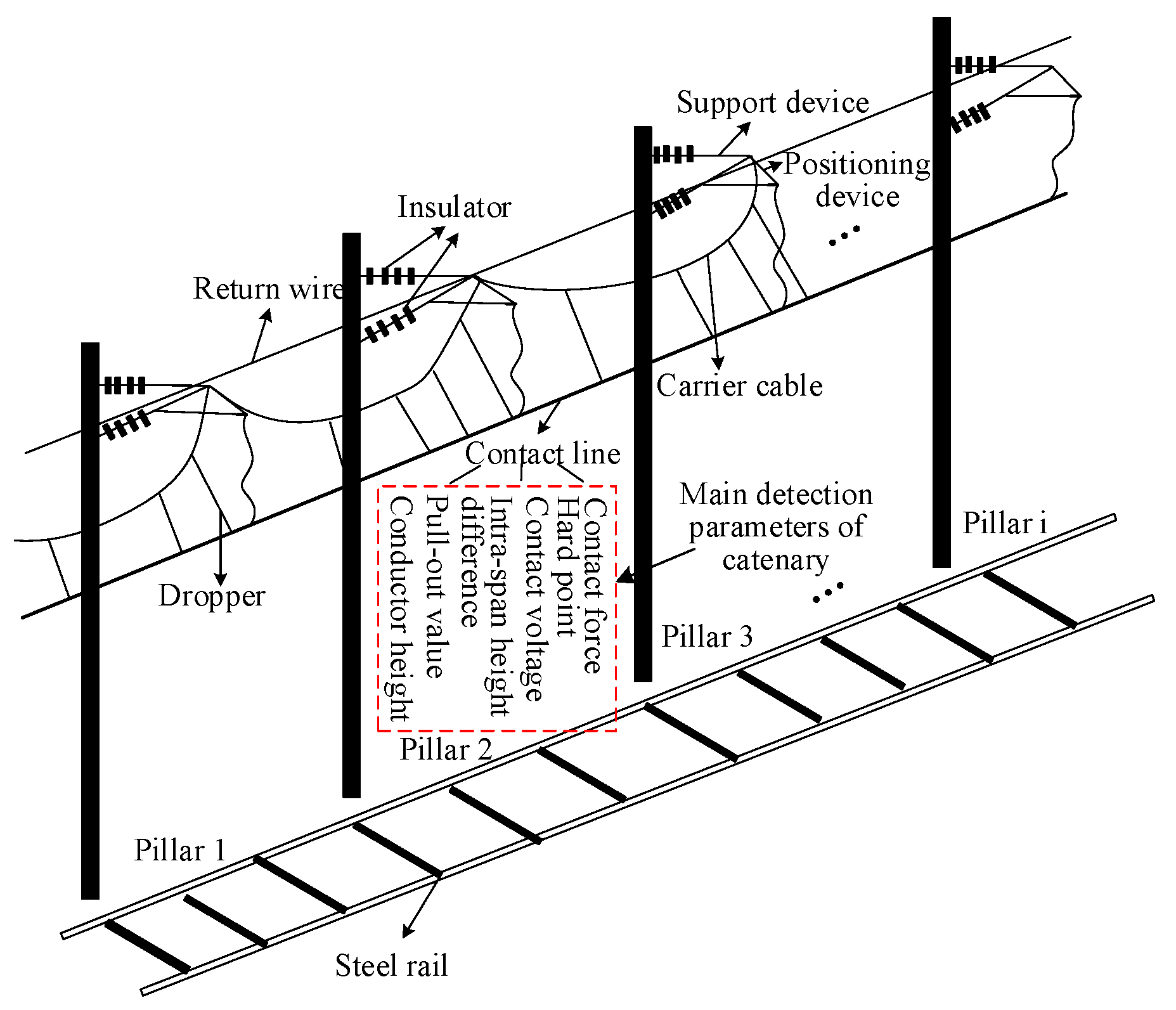
2. High-Speed Rail Catenary

The catenary is an important part of the railroad traction power supply system. It is set in an outdoor, open-air environment, has a harsh working environment, is easily influenced by the outside world and has a complex structure [31]. Therefore, it has become a subsystem with a high failure rate in the high-speed railroad system. The catenary’s primary structure and detection parameters are depicted in Figure 1.

It is apparent from Figure 1 that the high-speed rail catenary is a complex system with four main components that generally include contact suspension, support and positioning, pillars and foundations and electrical auxiliary equipment to ensure the safety of the equipment and the power supply [32].

Table 1. Description of the catenary’s primary detection parameters.

Parameter Name	Parameter Definition
Pull-out value (mm)	Lateral offset of the contact line at the detection point.
Conductor height (mm)	The vertical distance from the contact line at the detection point to the ground.
Intra-span height difference (mm)	The height difference of the contact line between the two pillars at the detection point.
Contact force (N)	The interaction force between the contact wire and the pantograph at the detection point.
Hard point (mm)	The location of the sudden change in contact pressure on the contact line.
Contact voltage (kV)	Voltage on the contact line at the detection point.

displays the primary parameters identified by the catenary comprehensive monitoring device.

The pull-out value may represent a component’s potential looseness or a pillar’s sideways tilt. The catenary’s smoothness can be seen in the conductor height and intra-span height difference. The quality of the power supply will be impacted, and there may even be arcing and line burnout due to hard point and excessive contact force, which will result in abnormal contact wear. Unusual contact voltage fluctuations will have an impact on how the electric multiple units operate. In conclusion, the pull-out value, conductor height, contact force, hard point, contact voltage and intra-span height difference are used to characterize the performance parameters of catenary systems.

The RUL is primarily determined using the project’s actual fault maintenance records. The inspection parameter values for each phase of the catenary with the same pillar number are assessed and compared to the inspection time point, using a specific catenary fault maintenance time point as the zero point of the RUL. To create a data set for the RUL of the catenary, the time difference is chosen as the RUL of the catenary’s pillar.

3. Model Design

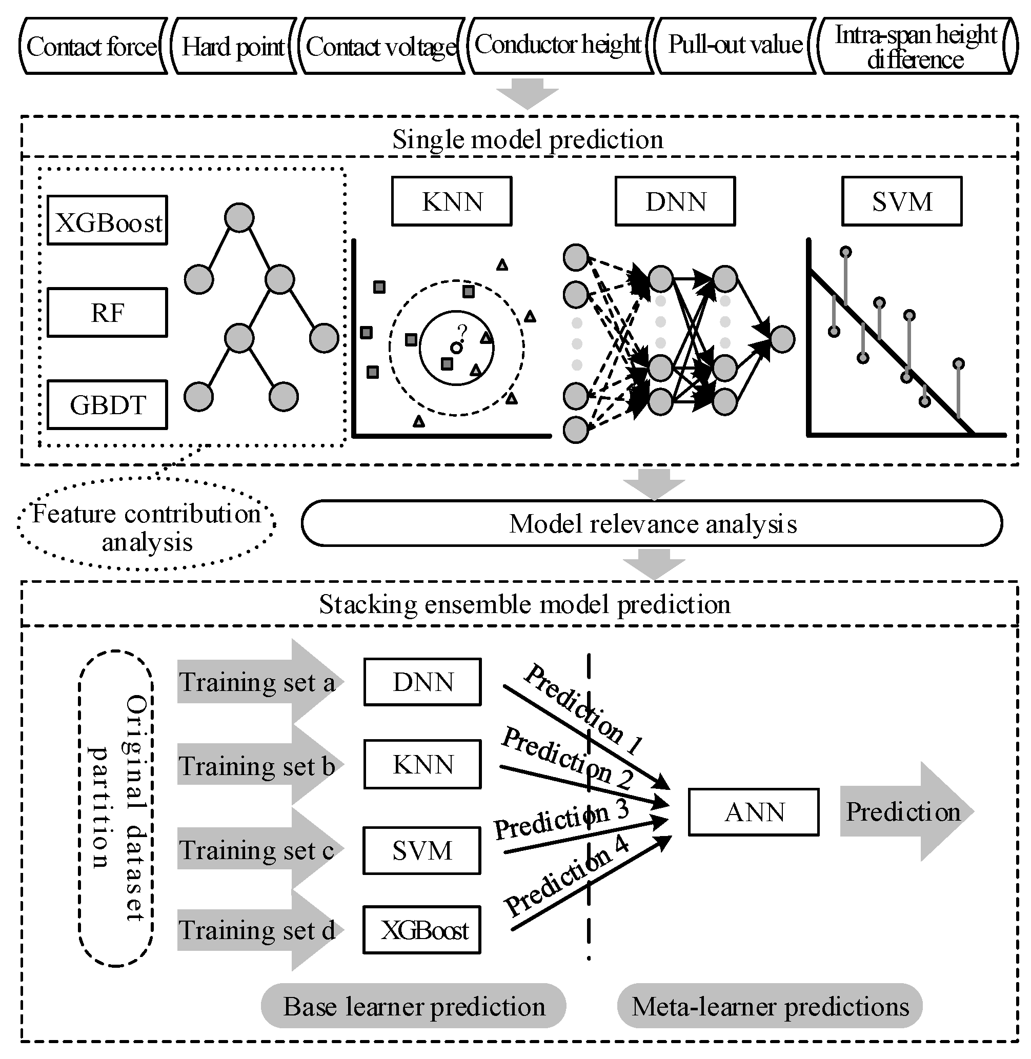
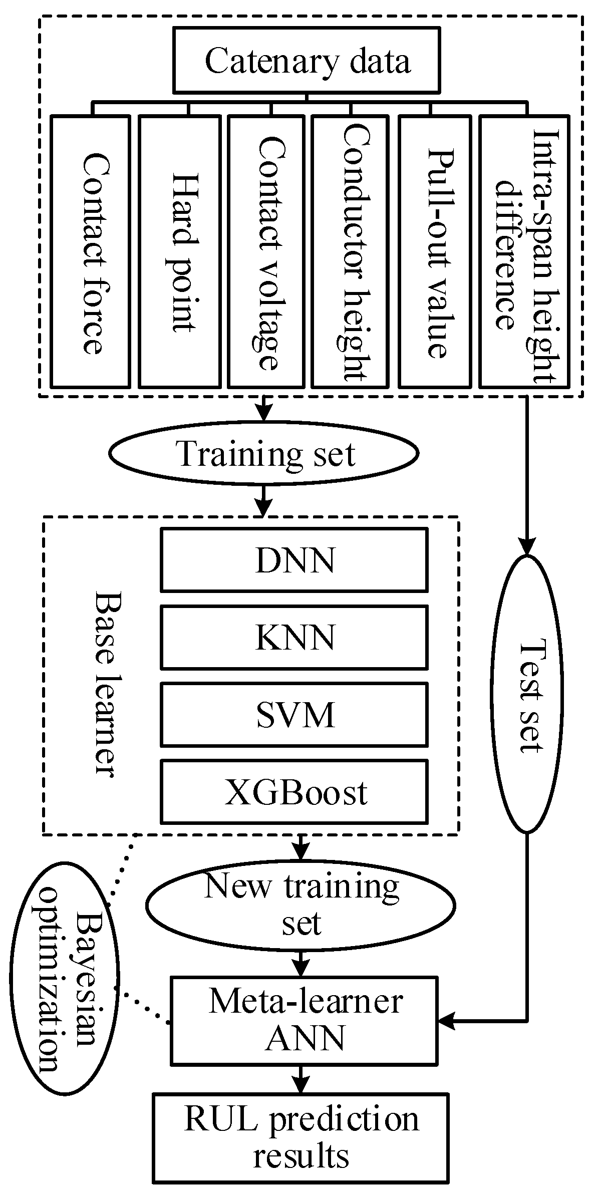
3.1. Design of the RUL Prediction Model

A stacking integration model is created with the goal of predicting the RUL of a catenary under multiple parameter conditions. In order to raise the RUL’s overall prediction accuracy, it fully utilizes the concept of multi-model fusion [33].

To guarantee the overall impact of the RUL prediction model, several algorithms with a better prediction performance should be chosen for the base model [34,35]. For instance, the integrated learning methods used by XGBoost, RF and the gradient boosting decision tree (GBDT), which have excellent prediction outcomes, are well-liked in many fields [36]. DNN is particularly effective in large-scale data analysis and solving nonlinear problems, making it a valuable addition to the base models for predicting the RUL. The SVM algorithm makes use of the kernel function to surmount the dimensionality and nonlinear separability problems, allowing for the successful prediction of a small sample. The KNN algorithm’s fundamental theory is developed, user-friendly and highly precise. In terms of machine learning, it is very representative. An RUL prediction model using the MLP algorithm for meta-learning has excellent generalization capabilities and can effectively combine the benefits of each basic learner to avoid the overfitting phenomenon. The RUL prediction model’s specific framework is shown in Figure 2.

Under the stacking integration framework, the RUL prediction method training proceeds as follows:

Step 1: Feature selection is a crucial step in constructing the model and can improve prediction accuracy by removing redundant features. Six parameters that significantly impact the performance of the catenary were manually selected, including the pull-out value, conductor height, contact force, hard point, contact voltage and intra-span height difference. The tree model’s special feature contribution calculation method was used to grade each feature, and useful features were chosen based on the XGBoost, GBDT and RF scoring results. Step 2: Catenary data was standardized using Formula (1) in order to mitigate the effects of dimensions between various features.

$$x^{\ast }=\frac{x-\min }{\max -\min }$$

(1)

where max represents the highest value among all the values prior to normalization, min represents the lowest value prior to normalization, x* represents the normalized value and x represents the value before normalization.

Step 3: The stacking integration model selected algorithms with significant differences in the first layer, allowing them to complement each other’s strengths and weaknesses. The Pearson correlation coefficient was used to determine the correlation level of each algorithm, and Formula (2) was used to calculate their correlation degree.

$$r_{ab}=\frac{{\displaystyle \sum _{i=1}^m\left(a_i-\overline{a}\right)\left(b_i-\overline{b}\right)}}{\sqrt{{\displaystyle \sum _{i=1}^m{\left(a_i-\overline{a}\right)}^2}}\sqrt{{\displaystyle \sum _{i=1}^m{\left(b_i-\overline{b}\right)}^2}}}$$

(2)

where a_i and b_i represent the ith error values of two distinct base learners, respectively, and $\overline{a}$ and $\overline{b}$ represent the average values of the error values of two distinct base learners.

Step 4: After K-fold cross validation, the data is divided into several parts and substituted into different base learners for training. The different prediction results generated by all base learners were re-integrated and trained as new input data. The training data of the substituted base learner and the meta learner were different, which effectively prevented the occurrence of over-fitting.

Step 5: The meta-learner was trained with the base learner’s prediction value as a feature vector, and it output the final prediction result.

In order to evaluate the effect of the remaining life prediction model, the root mean square error, mean absolute percentage error and mean absolute error in the following formula were selected to calculate the prediction accuracy of the model.

$$RMSE=\sqrt{\frac{1}{n}{\displaystyle \sum _{i=1}^n{\left(y-\widehat{y}\right)}^2}}$$

(3)

$$R^2=1-\frac{{\displaystyle \sum _{i=1}^n{\left(y-\widehat{y}\right)}^2}}{{\displaystyle \sum _{i=1}^n{\left(y-\overline{y}\right)}^2}}$$

(4)

$$MAE=\frac{1}{n}{\displaystyle \sum _{i=1}^n\left|y-\widehat{y}\right|}$$

(5)

where $\widehat{y}$ is the predicted RUL of the catenary; y is the actual RUL of the catenary; $\overline{y}$ is the average value of y; and n is the total number of samples for catenary RUL prediction.

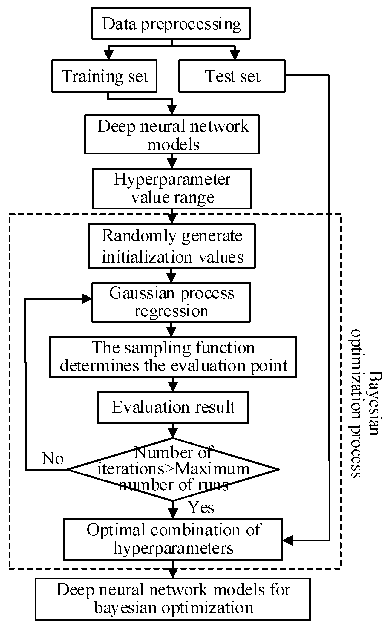
3.2. Bayesian Optimization Design

There are many parameters in machine learning or deep learning algorithms, and some of them, called hyperparameters, cannot be optimized through training and must instead be manually changed. Bayesian optimization can find a better parameter combination in fewer iterations than random search and grid search. As a result, the field of parameter optimization has been using Bayesian optimization algorithms frequently lately [37,38]. In order to find the most likely extreme point, the Bayesian optimization method continuously searches for the subsequent step based on the search results. The probabilistic surrogate model and the acquisition function are the two essential components of the Bayesian optimization method.

(1)

A surrogate model using probability.

A probabilistic surrogate model was used to roughly represent the current objective function. We were hopeful that the probabilistic surrogate model will begin with the initial a priori hypothesis and continuously add data information to the model to enhance it. Strong fitting capabilities make the Gaussian function a crucial component of the surrogate model, which can perform the modeling process iteratively. The parameter combination for a DNN model, for instance, that must be optimized is a Gaussian process, as in:

$$\{\begin{array}{l}f\left(x\right)\sim gp\left(m\left(x\right),k\left(x,x^{\prime }\right)\right)\hfill \\ m\left(x\right)=E\left[f\left(x\right)\right]\hfill \\ k\left(x,x^{\prime }\right)=E\left[\left(f\left(x\right)-m\left(x\right)\right)\left(f\left(x^{\prime }\right)-m\left(x^{\prime }\right)\right)\right]\hfill \end{array}$$

(6)

In the formula, m(x) is a function representing the mean value in order to simplify the calculation; m(x) = 0; k (x, x’) is a covariance function; f(x) ~ gp (0; k (x, x’)); the prior distribution of the unknown function can be expressed as p(f_1:t|D_1:t) ~ N(0, K_t); f_1:t is the value set of f, corresponding to the sampling point {f₁, f₂, …, f_t}; K_t is the covariance matrix formed by the covariance function, namely:

$$K_t=\left[\begin{array}{ccc}k\left(x_1,x_1\right)& \cdots & k\left(x_1,x_t\right)\\ ⋮& \ddots & ⋮\\ k\left(x_t,x_1\right)& \cdots & k\left(x_t,x_t\right)\end{array}\right]$$

(7)

When a new set of evaluation samples (x_t+1, f_t+1) is added to all evaluation point sets, the covariance matrix is updated as:

$$\{\begin{array}{l}{K}_{t+1}=\left[\begin{array}{l}{K}_t{k}_t{}^T\hfill \\ k_{t}k\left(x_{t+1},x_{t+1}\right)\hfill \end{array}\right]\hfill \\ k=\left[k\left(x,x\right),k\left(x,x\right),\cdots ,k\left(x,x\right)\right]\hfill \end{array}$$

(8)

The posterior probability distribution of f_t+1 is estimated using the updated covariance matrix, as shown in Formula (9):

$$\{\begin{array}{l}p\left(f_{t+1}|D_{1:t+1},x_{t+1}\right)\sim N\left(\mu ,{\sigma }^2\right)\hfill \\ \mu =k_{t+1}^T{K}_{t+1}^{-1}{f}_{1:t+1}\hfill \\ {\sigma }^2=k_{t+1}\left(x_{t+1},x_{t+1}\right)-k_{t+1}^T{K}_{t+1}^{-1}{k}_{t+1}\hfill \\ k_{t+1}=\left[k\left(x_{t+1},x_1\right),k\left(x_{t+1},x_2\right),\cdots ,k\left(x_{t+1},x_{t+1}\right)\right]\hfill \end{array}$$

(9)

(2)

Acquisition function

To obtain the subsequent sample point for analysis, the acquisition function was used. The probability of improvement (PI), expected improvement (EI) and upper confidence bound (UCB) are common acquisition functions. In this paper, the PI was chosen as the acquisition function. According to Formula (10), the PI represents the likelihood that the maximum value of the current objective function will increase when maximizing a new sample.

$${\alpha }_t\left(x;D_{1:t}\right)=p\left(f\left(x\right)\le {\upsilon }^{\ast }-\epsilon \right)=\phi \left(\frac{{\upsilon }^{\ast }-\epsilon -{\mu }_t\left(x\right)}{{\sigma }_t\left(x\right)}\right)$$

(10)

where υ* is the optimal value of the current objective function; φ(·) is the cumulative density function of the standard normal distribution; ε is the balance parameter.

For instance, Figure 3 illustrates how the Bayesian method and deep neural network hyperparameters are optimized.

To train models, the hyperparameters’ range of values was defined and various combinations of hyperparameters were chosen using Gaussian process regression. The hyperparameter combination that best fit the prediction requirements was chosen by comparing the model errors (MAE) of various hyperparameter combinations.

4. Experimental Verification

4.1. Dataset Preprocessing

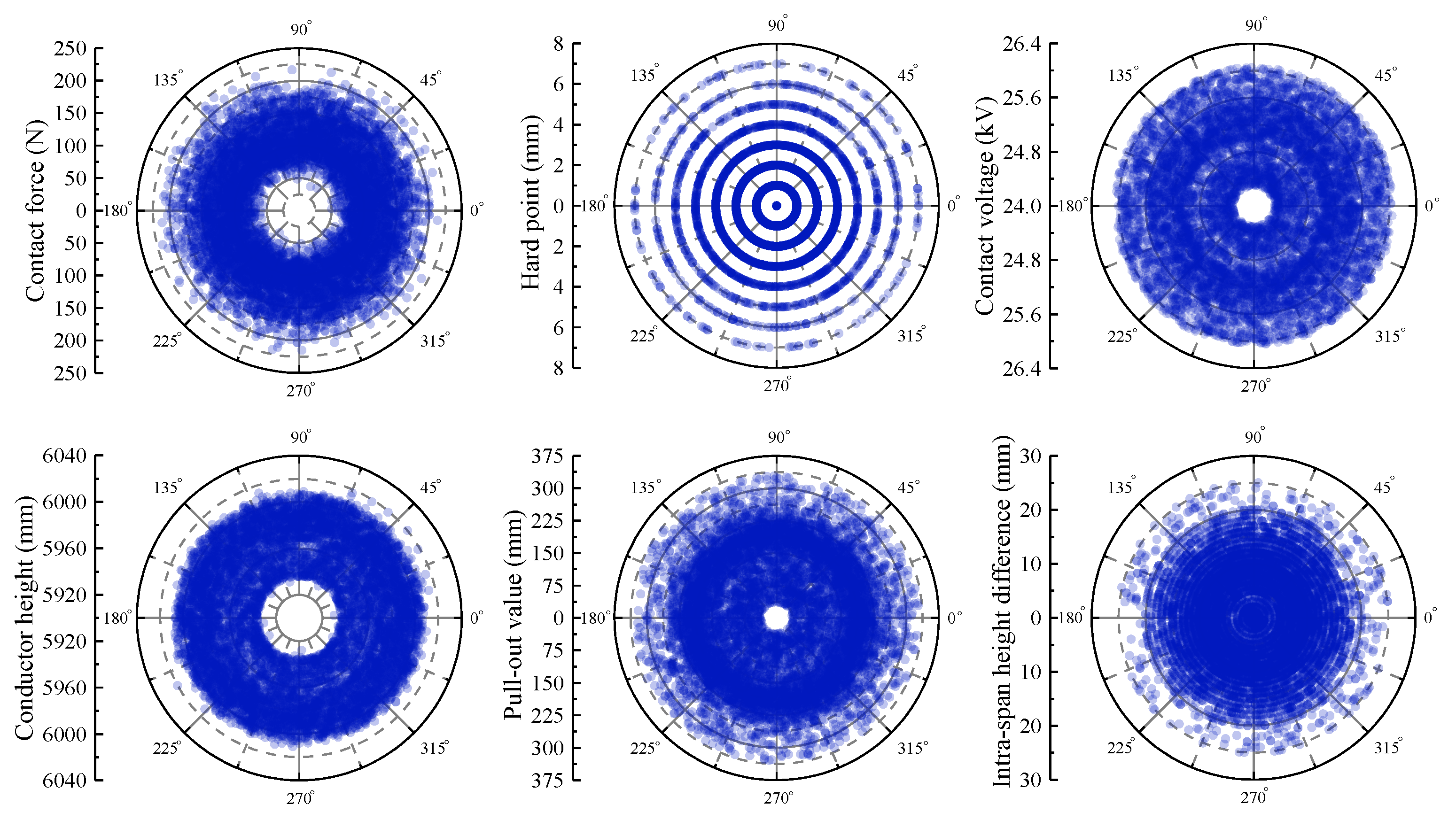
4.1.1. Catenary Dataset

This experiment selected the actual measurement data of a high-speed railway uplink and downlink catenary project in 2020, and the main parameter values of some data are shown in Figure 4.

The data were gathered by the railway power supply security detection and monitoring system, combined with the manual troubleshooting records, and cleaned. The data set contained one label, RUL, with a range of 0 to 172 days, and six attributes, including pull-out value, conductor height, contact force, hard point, contact voltage and intra-span height difference. The following is the attribute information:

(1)

Pull-out value: 36~330 mm

(2)

Conductor height: 5928~6020 mm

(3)

Contact force: 41~218 N

(4)

Hard point: 0~7 mm

(5)

Contact voltage: 24.30~26.05 kV

(6)

Intra-span height difference: 0~25 mm

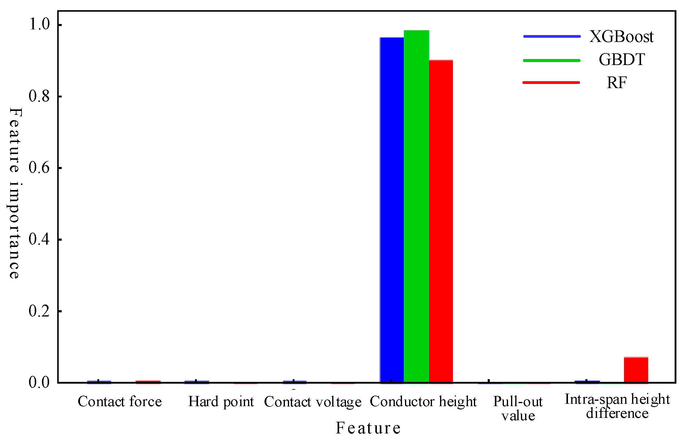
4.1.2. Feature Contribution Analysis

First, the standard contact force, hard point, contact voltage, conductor height, pull-out value and intra-span height difference were used as the model’s input data in accordance with manual experience. Figure 5 displays the feature contributions calculated by the XGBoost, GBDT and RF algorithms.

Among the attributes, the conductor height had the most influence on the prediction target, and the contact force, in-span height difference, contact voltage and pull-out value also had some influence on the RUL impact. While the hard point was coded with unique heat, the unique form of data made the measured contribution low; however, in the actual training of the model, the hard point data was still useful and the results of the feature selection had some reference value.

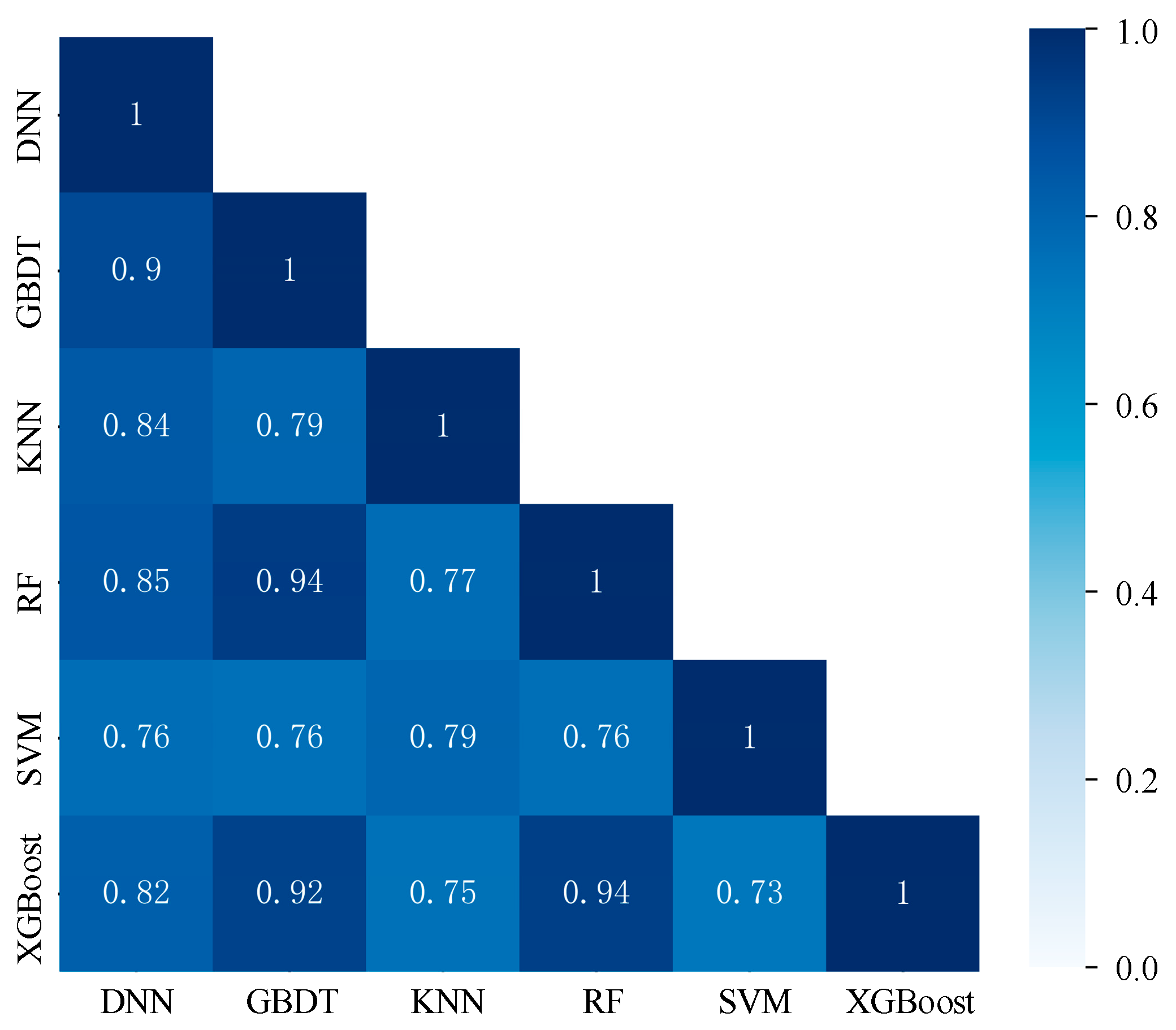
4.2. Correlation Analysis of Each Model

The learning capacity of the base model and the correlation between various base models needed to be examined in order to create a stacking integration model with better performance.

Prior to comparing and analyzing the predicted results, experiments were designed to train each base learner separately.

Table 2. Hyperparameter settings and prediction errors of XGBoost, SVM, RF, GBDT, KNN and DNN.

Method	Initial Hyperparameter Set	Single Model Prediction Error
		RMSE	R2	MAE
XGBoost	max depth: 8; learning rate: 0.05; n-estimators: 350; min child weight: 5; gamma: 0.05	0.095	0.914	0.080
SVM	kernel: poly; C: 2; gamma: 1; coef0: 0.01; degree: 1.5	0.098	0.909	0.080
RF	max depth: 6; n-estimators: 200; min samples leaf: 5; min samples split: 5	0.101	0.904	0.083
GBDT	max depth: 6; learning rate: 0.01; n-estimators: 150; min samples leaf: 10	0.106	0.895	0.090
KNN	n-neighbors: 3	0.108	0.890	0.080
DNN	hidden layers: 6; number of hidden layer kernels: 30; learning rate: 0.0001; activation: relu	0.113	0.881	0.091

displays the initial hyperparameter settings and prediction errors for each base learner.

Table 2 shows that when each algorithm made predictions independently, the error of the XGBoost algorithm’s prediction result was relatively small. This is because the XGBoost algorithm used Taylor’s second-order expansion to optimize the loss function and added a regular term to the objective function, which somewhat increased its prediction accuracy and generalization ability.

We evaluated and compared the prediction errors of the aforementioned single-model prediction results in order to choose the best base model combination for the RUL prediction model. To assess their correlation, a Pearson correlation coefficient value was chosen; the results are displayed in Figure 6.

From Figure 6, the error correlation coefficients of each algorithm were all over 0.7, which is typically high. This is due to the fact that each algorithm has a strong capacity for learning and can produce better prediction outcomes. However, the inherent errors in the data cannot be avoided throughout the learning process. Among them, the Pearson correlation coefficient of the XGBoost, GBDT and RF algorithms exceeded 0.9, with a high error correlation. This is due to the fact that even though the three algorithms differ slightly in concept, they all fall under the umbrella of the tree ensemble algorithm, and their approaches to data observation are very similar. The correlation coefficients of DNN, SVM and KNN Pearson were small, ranging from 0.7 to 0.9, due to the large differences in their training mechanisms. The selection criteria of stacking integration model meta-learners were thus satisfied by DNN, SVM and KNN.

4.3. Building the Stacking Integration Model

The base learner chose DNN, SVM and KNN with a Pearson correlation coefficient less than or equal to 0.9 and XGBoost, which performed the best in the tree integration model, in accordance with the difference degree of analysis of the example model. In order to eliminate overfitting and correct each base learner’s prediction bias, the meta-learner created an MLP model. Based on this, Figure 7 illustrates the stacking integration algorithm implementation process for obtaining the RUL of the high-speed rail catenary example system.

The dataset was first decomposed into multiple parts, and each part was fed into the appropriate base learner to produce appropriate predictions. Then, a fresh training set was created from its results and fed to the meta-learner for training. As a final step, the meta-learner’s output was used to determine the final prediction value.

4.4. Stacking Ensemble Algorithm Hyperparameter Optimization

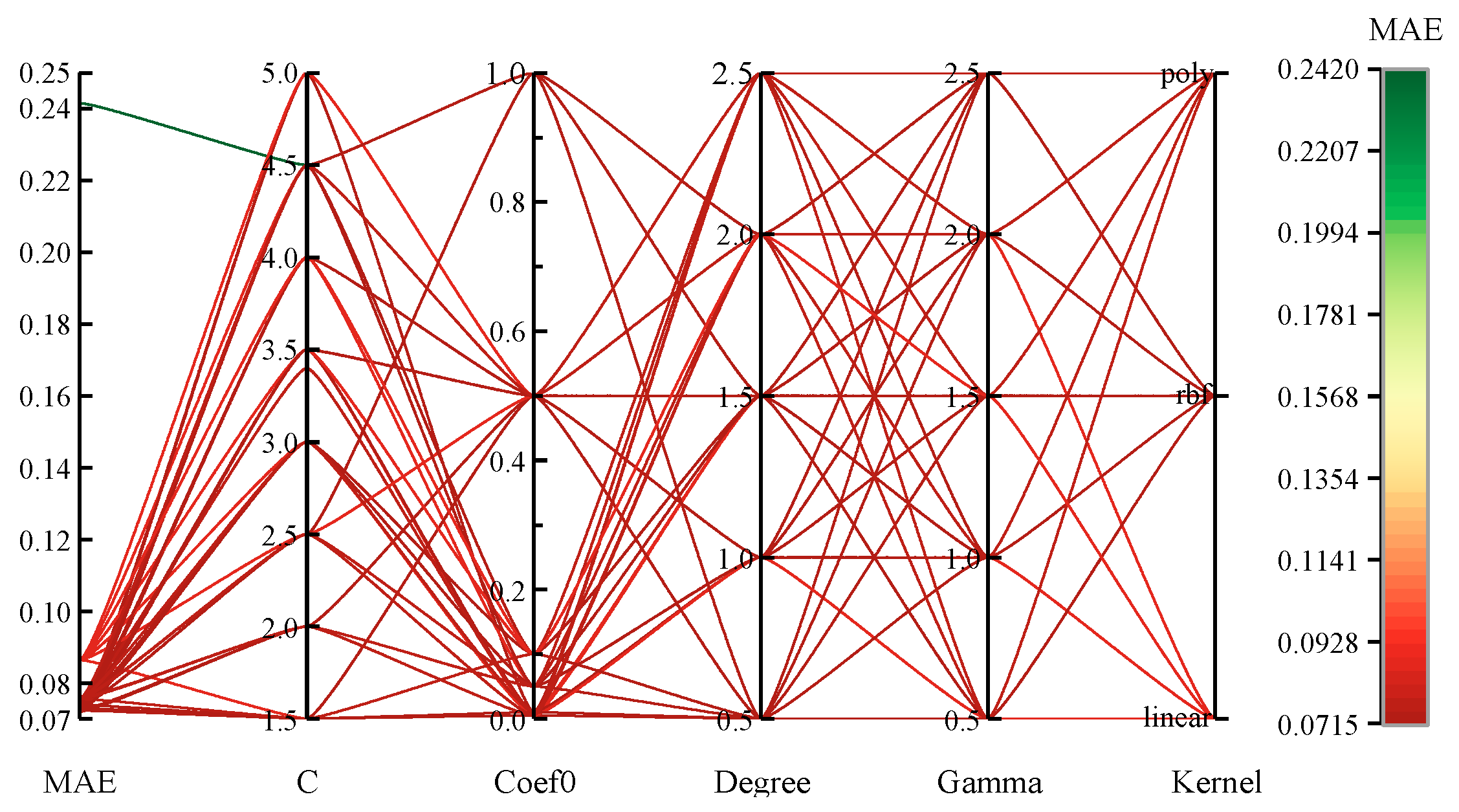
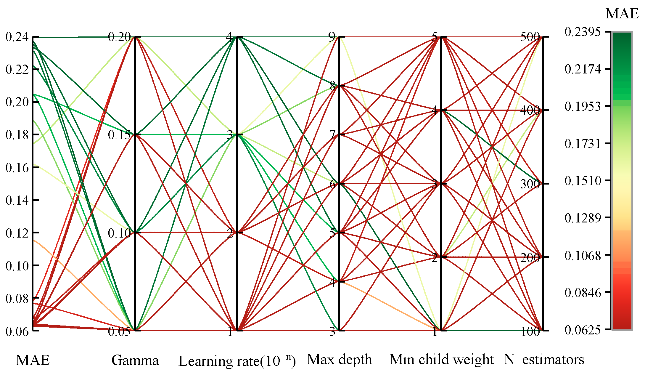
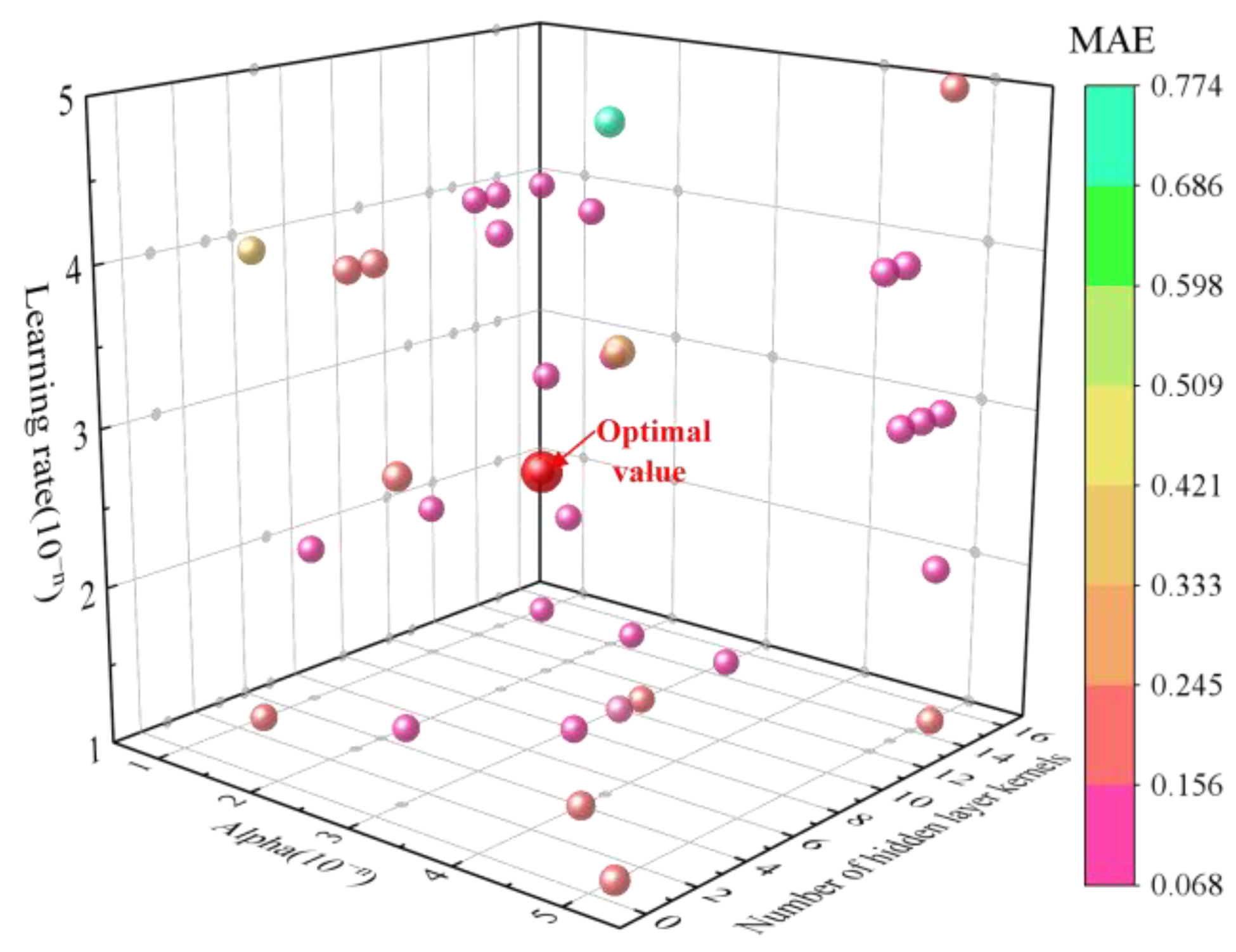
4.4.1. Choosing the Appropriate Hyperparameters for the Fundamental Learner

The learning rate, the number of hidden layers, the number of hidden layer kernels, the L2 regularization penalty coefficient, the batch size and the training times were the six hyperparameters chosen for optimization in the deep neural network used in the stacking integration algorithm. The value range and optimal combination of DNN hyperparameters are shown in

Table 3. Optimized hyperparameter types, meanings, ranges and optimal values of DNN.

Hyperparameter Category	Hyperparameter Meaning	Range	Optimal Value
Batch size	Training batch size	10, 20, 30, 40, 50	30
Times	Training times	100, 125, 150, 175, 200	200
Hidden layers	Number of hidden layers	1, 2, 3, 4, 5, 6, 7, 8, 9	6
L2	L2 regularization penalty coefficient	10−2, 10−3, 10−4, 10−5	10−4
Learning rate	Step size of model training	10−2, 10−3, 10−4, 10−5, 10−6	10−3
Kernels	Number of hidden layer kernels	10, 20, 30, 40, 50, 60, 70, 80, 90	70

, and the optimization process is shown in Figure 8.

The ideal set of hyperparameters was as follows: the learning rate was 0.001, the number of hidden layers was 6, the number of hidden layer kernels was 70, the L2 regularization penalty coefficient was 0.0001, the batch size was 30, and the training time was 200. Bayesian parameter tuning was used in this process to continuously update the prior by deriving the previous parameter information from an iteratively updating probability model.

The support vector machine model in the base learner selected five hyperparameters, such as C, for optimization. The initial hyperparameters of the model were also set to default values, and the evaluation standard was MAE. The value range and optimal combination of each hyperparameter are shown in

Table 4. Optimized hyperparameter types, meanings, ranges and optimal values of SVM.

Hyperparameter Category	Hyperparameter Meaning	Range	Optimal Value
C	Regularization parameter	1.5, 2, 2.5, 3, 3.5, 4, 4.5, 5	4
Coef0	Constant term of the kernel function	0.005, 0.05, 0.1, 0.5, 1	0.1
Degree	Dimensions of the polynomial poly function	0.5, 1, 1.5, 2, 2.5	0.5
Gamma	Coefficients of the kernel function	0.5, 1.5, 2, 2.5	1
Kernels	Type of kernel function	Poly, Rbf, Linear	Rbf

, and the optimization process is shown in Figure 9.

Continuous iteration caused the evaluation result of the hyperparameter combination to decline until the kernel was RBF, the C was 4, the gamma was 1, the coef0 was 0.1, and the degree was 0.5, at which point the model performed best.

The conventional hyperparameters, booster hyperparameters and task parameters were the three main categories of hyperparameters in the XGBoost model. To achieve the goal of optimizing the model performance, it was necessary to appropriately adjust the booster hyperparameters because the conventional hyperparameters and task parameters typically use the default values. The value range and optimal combination of XGBoost hyperparameters are shown in

Table 5. Optimized hyperparameter types, meanings, ranges and optimal values of XGBoost.

Hyperparameter Category	Hyperparameter Meaning	Range	Optimal Value
Gamma	Minimum loss reduction required to make a further partition on a leaf node of the tree	0.05, 0.1, 0.15, 0.2	0.05
Learning rate	Step size of model training	10−1, 10−2, 10−3, 10−4	10−1
Max depth	Maximum depth of a tree	3, 4, 5, 6, 7, 8, 9	5
Min child weight	Minimum sum of instance weight needed in a child	1, 2, 3, 4, 5	3
N-estimators	Total number of iterations	100, 200, 300, 400, 500	400

, and the optimization process is shown in Figure 10.

The ideal set of hyperparameters was as follows: the gamma value was 0.05, the learning rate was 0.1, maximum depth was 5, the n-estimators value was 400, and the minimum child weight was 3.

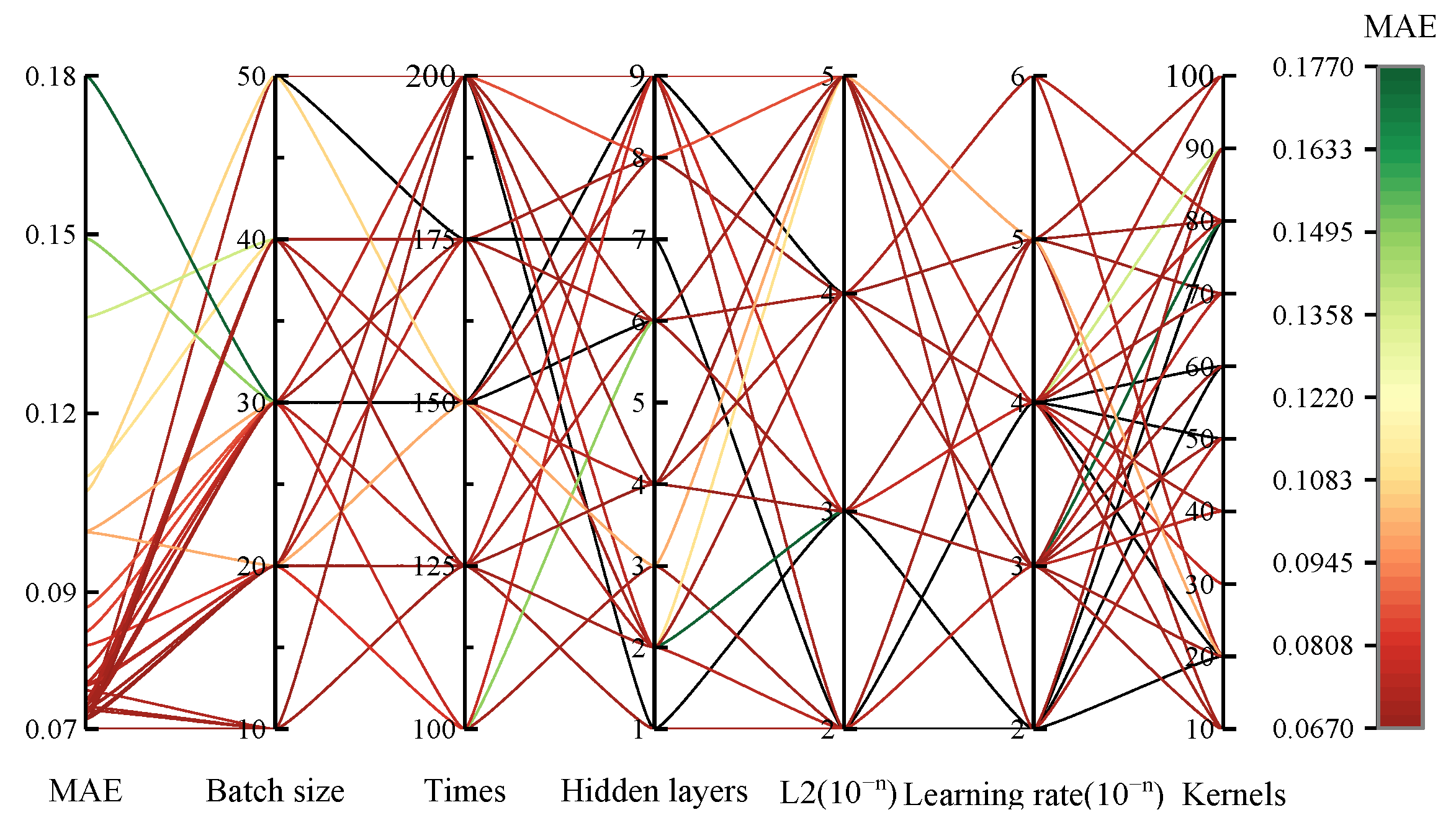
4.4.2. Hyperparameter Selection for Meta-Learners

The learning rate, alpha and number of hidden layer kernels were the three categories of hyperparameter that the MLP model chose for optimization. Figure 11 depicts the optimization process and the range of values for the hyperparameters.

Finally, the result of the Bayesian optimization was a learning rate of 0.01, an alpha of 0.1, and the number of hidden layer kernels was 15.

5. Analysis and Comparison

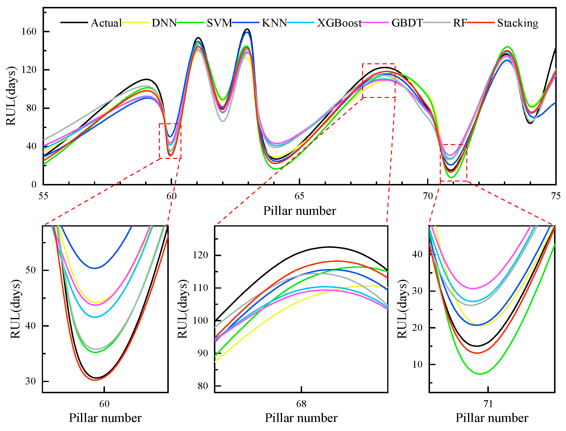
5.1. Comparison of the Stacking Model’s Prediction Outcomes with Those of Other Models

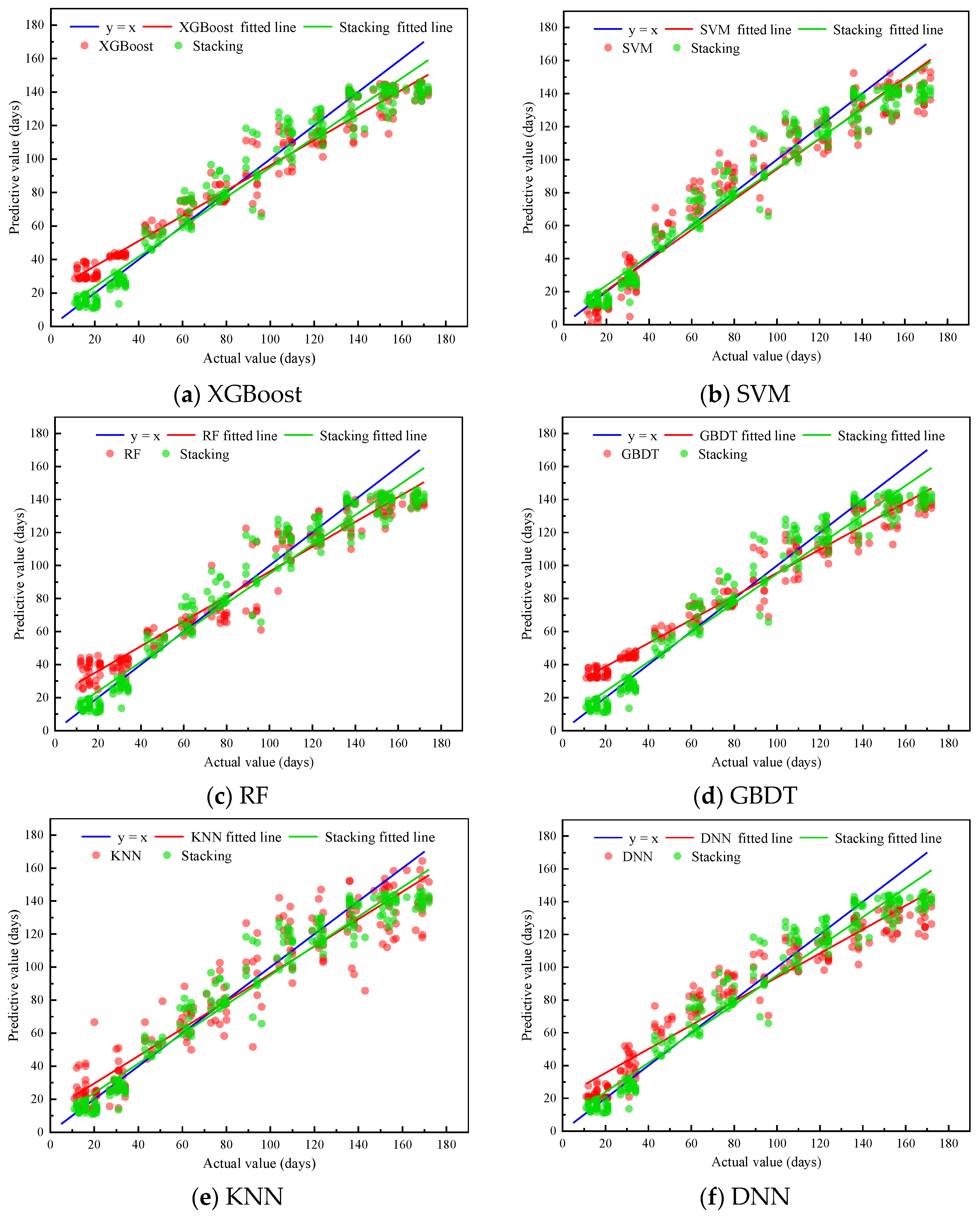
5.1.1. Comparison Using Just One Model

The pre-processed contact network data were fed into stacking integration remaining life prediction algorithm, and some of the output prediction results are shown in Figure 12. The stacking prediction outcomes are more in line with the actual values.

The prediction results of single models (XGBoost, DNN, GBDT, RF, SVM and KNN) and stacking integration model were compared one by one to further analyze the performance of stacking integration model, and the comparison results are shown in Figure 13.

Figure 13 demonstrates the stark differences in the shapes of the RUL prediction curves between the stacking, XGBoost, SVM, RF, GBDT, KNN and DNN models. The predicted value of the stacking integration model is also more similar to the real value. The stacking integration model presents a more excellent overall effect because it not only fully exploits the strengths of each base learner but also breaks the connection with a subpar prediction effect. Training a single model, on the other hand, has a tendency to result in a local minimum. However, by fusing several models, it is possible to significantly lower the likelihood of this happening and increase the generalizability of the final model.

Table 6. Prediction error stacking for various base learner combinations.

Basic Learner Combination	RMSE	R2	MAE
XGBoost	0.095	0.914	0.080
SVM	0.098	0.909	0.080
RF	0.101	0.904	0.083
GBDT	0.106	0.895	0.090
KNN	0.108	0.890	0.080
DNN	0.113	0.881	0.091
Stacking	0.080	0.940	0.059

shows the evaluation index values (RMSE, R² and MAE) of the XGBoost, SVM, RF, GBDT, KNN, DNN and stacking models.

It can be seen from Table 6 that the RMSE value and MAE value of the stacking integration model are smaller, 0.033 lower than the lowest RMSE value of the other models. Additionally, the lowest MAE value is 0.032 smaller, and the prediction error has been significantly reduced. The R² of the stacking integration model is larger than other models, which also means that the prediction accuracy of the model is higher.

5.1.2. Comparison and Analysis of Stacking Models with Various Base Learners

The general prediction effect is somewhat influenced by the base learner. The prediction error values for the models trained with various base learner combinations are shown in

Table 7. Prediction error stacking for various base learner combinations.

Basic Learner Combination	RMSE	R2	MAE
XGBoost, DNN, SVM, KNN	0.080	0.940	0.059
GBDT, SVM, KNN	0.083	0.935	0.063
RF, KNN	0.089	0.926	0.070
GBDT, DNN, SVR, KNN	0.090	0.924	0.070
DNN, SVM, KNN	0.095	0.915	0.073

.

The prediction results demonstrate that the choice of different base learners significantly affects the outcome of the prediction, and that the stacking model using the base learner with the minimum correlation outperforms the stacking model using the base learner chosen at random. On the one hand, the fusion model performs significantly better when the base learner is excellent. On the other hand, the variation in the base learners allows the integration results to benefit from one another, resulting in a more consistent and precise effect.

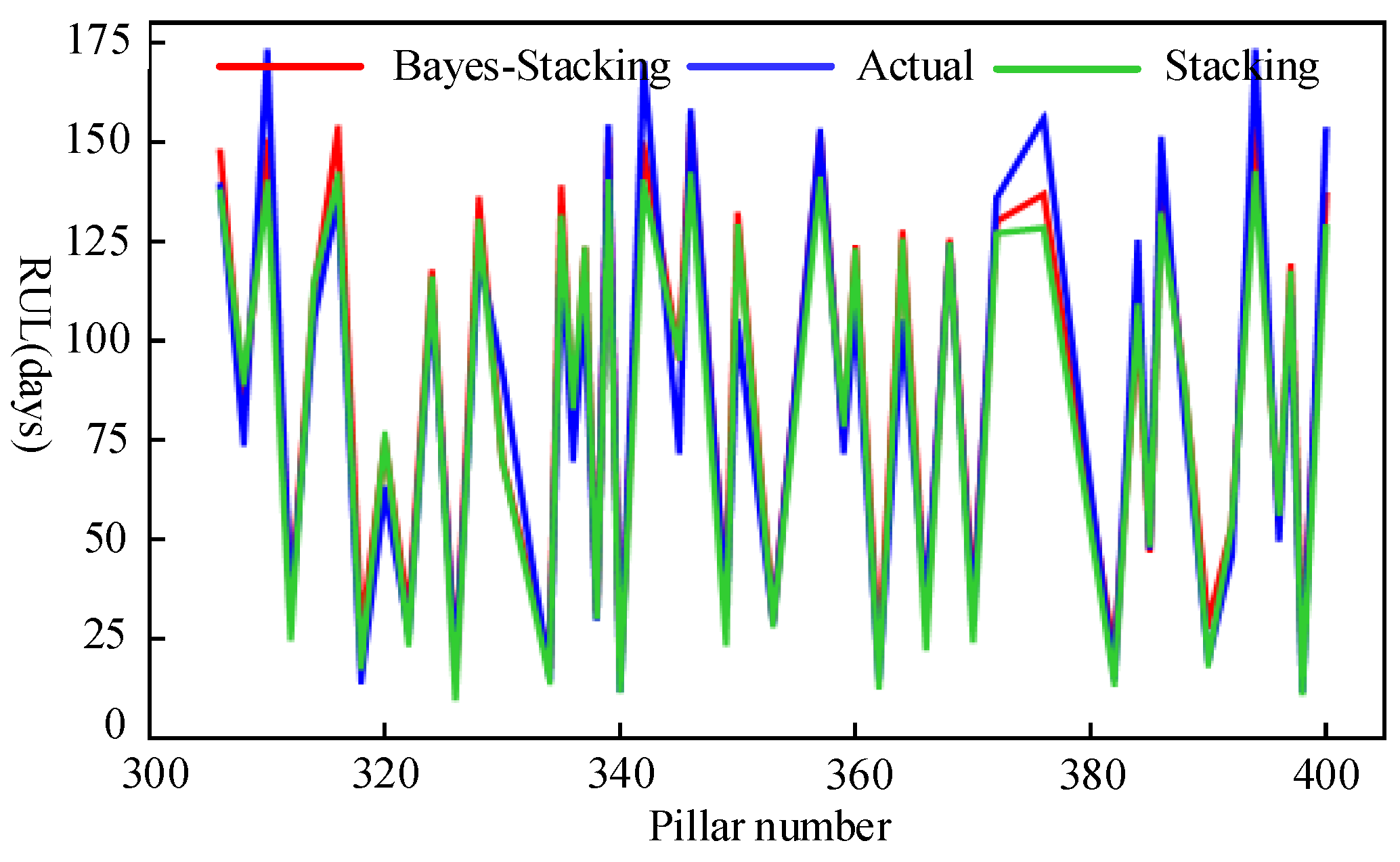
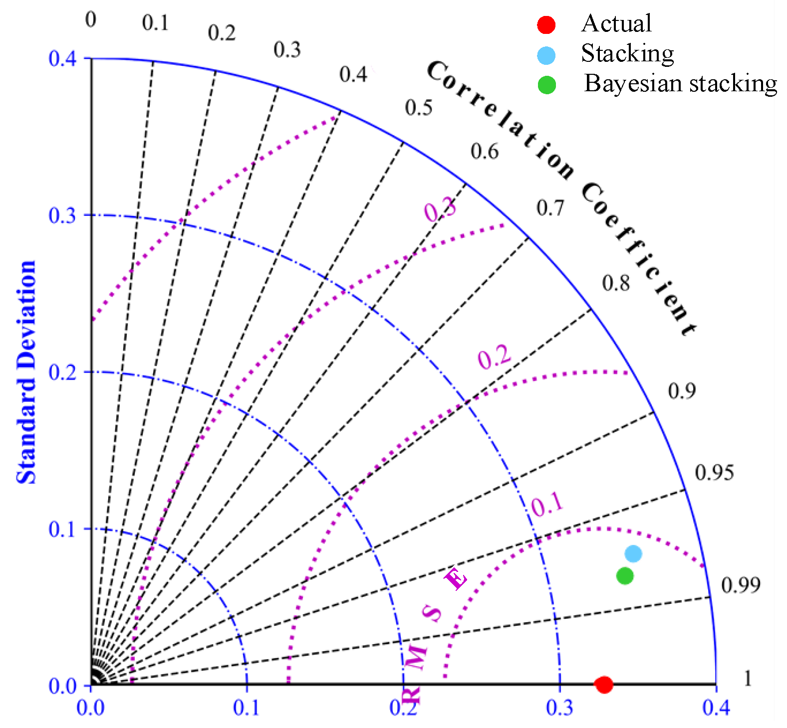
5.2. Results of Stacking Model Hyperparameter Optimization Are Analyzed and Compared

The comparison of the obtained prediction results is shown in Figure 14 after the hyperparameter combination optimized by the Bayesian method was substituted into the stacking integrated model for re-experimentation.

The RUL predicted value of the optimized stacking integrated model is more in line with the actual value, and the model’s accuracy both before and after optimization is enhanced. After Bayesian optimization, the RMSE and MAE decreased by 15% and 10.17%, and the R² increased by 1.81%. By using the three indicators of standard deviation, root mean square deviation and correlation coefficient, you can further compare the accuracy of the model before and after optimization by creating a Taylor diagram.

Figure 15 demonstrates that the Bayesian-optimized stacking integration algorithm’s predicted value is more in line with the actual value, demonstrating that the Bayesian-optimized stacking model has a better predictive effect.

6. Conclusions

Aimed at addressing the problem of the low maintenance efficiency of a high-speed rail catenary, a stacking ensemble algorithm based on Bayesian optimization was designed to predict the RUL of the catenary. Through an accurate life prediction, it provides a data basis for formulating detailed and timely maintenance plans. The numerical example test demonstrates that the analysis of the feature contribution before the model is established can clearly show the quantitative value of the importance of each feature. The XGBoost, DNN, SVM and KNN components of the stacking ensemble learning algorithm have good RUL prediction accuracy. The prediction error evaluation index (RMSE) after optimization using the Bayesian approach is 0.068, the R² is 0.957 and the MAE is 0.053. It has significant application value in the prediction of the RUL of the catenary and produces prediction results that are more accurate than those of a single conventional machine learning algorithm.

Due to the diversity of the natural environment in which the catenary is located, the research on the catenary must use data from different regions to enhance its universality. Based on the catenary data of a specific line, the weight coefficient values and offset vector values of each algorithm obtained in this paper are only applicable to the remaining useful life prediction of special lines. Therefore, for different lines, it is necessary to use different detection data to correct the weight coefficient and the offset vector.

Future work will focus more on the application of artificial intelligence technology in high-speed electrified railway transportation systems and other aspects. In addition, the use of enhancing technologies such as building information modeling in high-speed railway transportation systems will carry out more in-depth planned and reactive maintenance cost analyses.

(1)

The stacking, two-layer framework is computationally expensive due to its complexity and the need for many trained models. The decomposition of the training model into numerous minor components for independent processing using distributed computing significantly increases the computing efficiency.

(2)

AI technology has improved the failure and RUL prediction at the application level [39]. Future high-speed rail system development will focus on fault prediction and health management, and the combination of deep learning and high-speed rail system prediction will continue to be extremely valuable.

(3)

Building information modeling (BIM) also has the potential to reduce planned and reactive high-speed rail catenary maintenance costs, thus in-creasing the RUL prediction of a high-speed rail catenary.

References

1. Feng, D.; He, Z.Y.; Lin, S.; Wang, Z.; Sun, X.J. Risk index system for catenary lines of high-speed railway considering the characteristics of time-space differences. IEEE Trans. Transp. Electrif. 2017, 3, 739–749. [Google Scholar] [CrossRef]
2. Guo, L.; Gao, X.J.; Li, Q.Z.; Huang, W.X.; Shu, Z.L. Online antiicing technique for the catenary of the high-speed electric railway. IEEE Trans. Power Deliv. 2015, 30, 1569–1576. [Google Scholar] [CrossRef]
3. Qin, Y.; Xiao, S.; Lu, L.; Yang, B.; Zhu, T.; Yang, G. Fatigue failure of integral droppers of high-speed railway catenary under impact load. Eng. Fail. Anal. 2022, 134, 106086. [Google Scholar] [CrossRef]
4. Moghaddass, R.; Zuo, M.J. An integrated framework for online diagnostic and prognostic health monitoring using a multistate deterioration process. Reliab. Eng. Syst. Saf. 2014, 124, 92–104. [Google Scholar] [CrossRef]
5. Elsheikh, A.; Yacout, S.; Ouali, M.-S. Bidirectional handshaking LSTM for remaining useful life prediction. Neurocomputing 2019, 323, 148–156. [Google Scholar] [CrossRef]
6. Xu, X.; Wu, Q.; Li, X.; Huang, B. Dilated convolution neural network for remaining useful life prediction. J. Comput. Inf. Sci. Eng. 2020, 20, 021004. [Google Scholar] [CrossRef]
7. Sikorska, J.Z.; Hodkiewicz, M.; Ma, L.J.M.S.; Processing, S. Prognostic modelling options for remaining useful life estimation by industry. Mech. Syst. Signal Process. 2011, 25, 1803–1836. [Google Scholar] [CrossRef]
8. Wang, Y.W.; Gogu, C.; Binaud, N.; Bes, C.; Haftka, R.T.; Kim, N.H. Predictive airframe maintenance strategies using model-based prognostics. Proc. Inst. Mech. Eng. Part O-J. Risk Reliab. 2018, 232, 690–709. [Google Scholar] [CrossRef]
9. Cai, Z.Y.; Wang, Z.Z.; Chen, Y.X.; Guo, J.S.; Xiang, H.C. Remaining useful lifetime prediction for equipment based on nonlinear implicit degradation modeling. J. Syst. Eng. Electron. 2020, 31, 194–205. [Google Scholar] [CrossRef]
10. Li, N.; Lei, Y.; Gebraeel, N.; Wang, Z.; Cai, X.; Xu, P.; Wang, B. Multi-sensor data-driven remaining useful life prediction of semi-observable systems. IEEE Trans. Ind. Electron. 2021, 68, 11482–11491. [Google Scholar] [CrossRef]
11. Wu, J.; Hu, K.; Cheng, Y.; Zhu, H.; Shao, X.; Wang, Y. Data-driven remaining useful life prediction via multiple sensor signals and deep long short-term memory neural network. ISA Trans. 2020, 97, 241–250. [Google Scholar] [CrossRef] [PubMed]
12. Cai, B.P.; Shao, X.Y.; Liu, Y.H.; Kong, X.D.; Wang, H.F.; Xu, H.Q.; Ge, W.F. Remaining useful life estimation of structure systems under the influence of multiple causes: Subsea pipelines as a case study. IEEE Trans. Ind. Electron. 2020, 67, 5737–5747. [Google Scholar] [CrossRef]
13. Chen, Z.H.; Wu, M.; Zhao, R.; Guretno, F.; Yan, R.Q.; Li, X.L. Machine remaining useful life prediction via an attention-based deep learning approach. IEEE Trans. Ind. Electron. 2021, 68, 2521–2531. [Google Scholar] [CrossRef]
14. Sunar, Ö.; Fletcher, D. A new small sample test configuration for fatigue life estimation of overhead contact wires. Proc. Inst. Mech. Eng. Part F J. Rail Rapid Transit 2022, 237, 438–444. [Google Scholar] [CrossRef]
15. Zhao, R.; Yan, R.Q.; Wang, J.J.; Mao, K.Z. Learning to monitor machine health with convolutional bi-directional LSTM networks. Sensors 2017, 17, 273. [Google Scholar] [CrossRef] [Green Version]
16. Rahimi, A.; Kumar, K.D.; Alighanbari, H. Failure prognosis for satellite reaction wheels using kalman filter and particle filter. J. Guid. Control. Dyn. 2020, 43, 585–588. [Google Scholar] [CrossRef]
17. Guo, R.X.; Sui, J.F. Remaining useful life prognostics for the electrohydraulic servo actuator using hellinger distance-based particle filter. IEEE Trans. Instrum. Meas. 2020, 69, 1148–1158. [Google Scholar] [CrossRef]
18. Zan, T.; Liu, Z.; Wang, H.; Wang, M.; Gao, X.; Pang, Z. Prediction of performance deterioration of rolling bearing based on JADE and PSO-SVM. Proc. Inst. Mech. Eng. 2020, 235, 1684–1697. [Google Scholar] [CrossRef]
19. Zhen, L.; Wenjuan, M.; Xianping, Z.; Chenglin, Y.; Xiuyun, Z.J.S. Remaining useful life estimation of insulated gate biploar transistors (IGBTs) based on a novel volterra k-nearest neighbor optimally pruned extreme learning machine (VKOPP) model using degradation data. Sensors 2017, 17, 2524. [Google Scholar] [CrossRef] [Green Version]
20. Zhang, Y.; Peng, Z.; Guan, Y.; Wu, L.J.E. Prognostics of battery cycle life in the early-cycle stage based on hybrid model. Energy 2021, 221, 119901. [Google Scholar] [CrossRef]
21. Reddy Maddikunta, P.K.; Srivastava, G.; Reddy Gadekallu, T.; Deepa, N.; Boopathy, P. Predictive model for battery life in IoT networks. IET Intell. Transp. Syst. 2020, 14, 1388–1395. [Google Scholar] [CrossRef]
22. Gupta, M.; Kumar, N.; Singh, B.K.; Gupta, N.; Damaševičius, R. NSGA-III-based deep-learning model for biomedical search engines. Math. Probl. Eng. 2021, 2021, 1–8. [Google Scholar] [CrossRef]
23. Kodepogu, K.R.; Annam, J.R.; Vipparla, A.; Krishna, B.V.N.V.S.; Kumar, N.; Viswanathan, R.; Gaddala, L.K.; Chandanapalli, S.K. A novel deep convolutional neural network for diagnosis of skin disease. Trait. Du Signal 2022, 39, 1873–1877. [Google Scholar] [CrossRef]
24. Liu, H.; Liu, Z.Y.; Jia, W.Q.; Lin, X.K. Remaining useful life prediction using a novel feature-attention-based end-to-end approach. IEEE Trans. Ind. Inform. 2021, 17, 1197–1207. [Google Scholar] [CrossRef]
25. Yi, L.; Zhao, J.; Yu, W.; Long, G.; Sun, H.; Li, W. Health status evaluation of catenary based on normal fuzzy matter-element and game theory. J. Electr. Eng. Technol. 2020, 15, 2373–2385. [Google Scholar] [CrossRef]
26. Wang, P.; Qin, J.; Li, J.; Wu, M.; Zhou, S.; Feng, L. Device status evaluation method based on deep learning for PHM scenarios. Electronics 2023, 12, 779. [Google Scholar] [CrossRef]
27. Wang, H.R.; Nunez, A.; Liu, Z.G.; Zhang, D.L.; Dollevoet, R. A bayesian network approach for condition monitoring of high-speed railway catenaries. IEEE Trans. Intell. Transp. Syst. 2020, 21, 4037–4051. [Google Scholar] [CrossRef]
28. Qu, Z.J.; Yuan, S.G.; Chi, R.; Chang, L.C.; Zhao, L. Genetic optimization method of pantograph and catenary comprehensive monitor status prediction model based on adadelta deep neural network. IEEE Access 2019, 7, 23210–23221. [Google Scholar] [CrossRef]
29. Awang, M.K.; Makhtar, M.; Udin, N.; Mansor, N.F. Improving customer churn classification with ensemble stacking method. Int. J. Adv. Comput. Sci. Appl. 2021, 12, 277. [Google Scholar] [CrossRef]
30. Agrawal, S.; Sarkar, S.; Srivastava, G.; Maddikunta, P.K.R.; Gadekallu, T.R. Genetically optimized prediction of remaining useful life. Sustain. Comput. Inform. Syst. 2021, 31, 100565. [Google Scholar] [CrossRef]
31. Li, B.; Cui, F. Inception module and deep residual shrinkage network-based arc fault detection method for pantograph–catenary systems. J. Power Electron. 2022, 22, 991–1000. [Google Scholar] [CrossRef]
32. Jiang, T.; Rønnquist, A.; Song, Y.; Frøseth, G.T.; Nåvik, P. A detailed investigation of uplift and damping of a railway catenary span in traffic using a vision-based line-tracking system. J. Sound Vib. 2022, 527, 116875. [Google Scholar] [CrossRef]
33. Oleiwi, H.W.; Mhawi, D.N.; Al-Raweshidy, H. A meta-model to predict and detect malicious activities in 6G-structured wireless communication networks. Electronics 2023, 12, 643. [Google Scholar] [CrossRef]
34. Dong, Y.; Zhang, H.; Wang, C.; Zhou, X. Wind power forecasting based on stacking ensemble model, decomposition and intelligent optimization algorithm. Neurocomputing 2021, 462, 169–184. [Google Scholar] [CrossRef]
35. Pinto, T.; Praça, I.; Vale, Z.; Silva, J. Ensemble learning for electricity consumption forecasting in office buildings. Neurocomputing 2021, 423, 747–755. [Google Scholar] [CrossRef]
36. Torres-Barrán, A.; Alonso, Á.; Dorronsoro, J.R. Regression tree ensembles for wind energy and solar radiation prediction. Neurocomputing 2019, 326, 151–160. [Google Scholar] [CrossRef]
37. Shin, S.; Lee, Y.; Kim, M.; Park, J.; Lee, S.; Min, K. Deep neural network model with Bayesian hyperparameter optimization for prediction of NOx at transient conditions in a diesel engine. Eng. Appl. Artif. Intell. 2020, 94, 103761. [Google Scholar] [CrossRef]
38. Sun, J.; Wu, S.; Zhang, H.; Zhang, X.; Wang, T. Based on multi-algorithm hybrid method to predict the slope safety factor-- stacking ensemble learning with bayesian optimization. J. Comput. Sci. 2022, 59, 101587. [Google Scholar] [CrossRef]
39. Kumar, N.; Hashmi, A.; Gupta, M.; Kundu, A. Automatic diagnosis of Covid-19 related pneumonia from CXR and CT-Scan images. Eng. Technol. Appl. Sci. Res. 2022, 12, 7993–7997. [Google Scholar] [CrossRef]
Figure 1. Catenary’s primary composition and detection capabilities.
Electronics 12 01744 g001
Figure 2. Design architecture of the RUL prediction model.
Electronics 12 01744 g002
Figure 3. Bayesian optimized deep neural network model.
Electronics 12 01744 g003
Figure 4. Some historical detection data of a catenary.
Electronics 12 01744 g004
Figure 5. An examination of how various algorithms contribute to features.
Electronics 12 01744 g005
Figure 6. Comparison of prediction error correlations for each single model.
Electronics 12 01744 g006
Figure 7. The final model of the RUL of the high-speed rail catenary under the stacking framework.
Electronics 12 01744 g007
Figure 8. Optimization of DNN hyperparameters.
Electronics 12 01744 g008
Figure 9. Process for optimizing SVM hyperparameters.
Electronics 12 01744 g009
Figure 10. Hyperparameter optimization process for XGBoost.
Electronics 12 01744 g010
Figure 11. Process for optimizing MLP hyperparameters.
Electronics 12 01744 g011
Figure 12. Comparison of predicted and actual values for DNN, SVM, KNN, XGBoost, GBDT, RF and stacking.
Electronics 12 01744 g012
Figure 13. Comparison of the prediction errors produced by the XGBoost, SVM, RF, GBDT, KNN, DNN and stacking models.
Electronics 12 01744 g013
Figure 14. Before and after Bayesian hyperparameter optimization, a comparison of the model’s predicted value and the actual value was made.
Electronics 12 01744 g014
Figure 15. Before and after results of integrated model prediction stacking, according to a Taylor diagram.
Electronics 12 01744 g015