
An Air Pollutant Forecast Correction Model Based on Ensemble Learning Algorithm


Abstract
1. Introduction
- (1)
- (2)
2. Related Work
3. Methodology
3.1. Bagging Ensemble Method
3.2. Boosting Ensemble Method
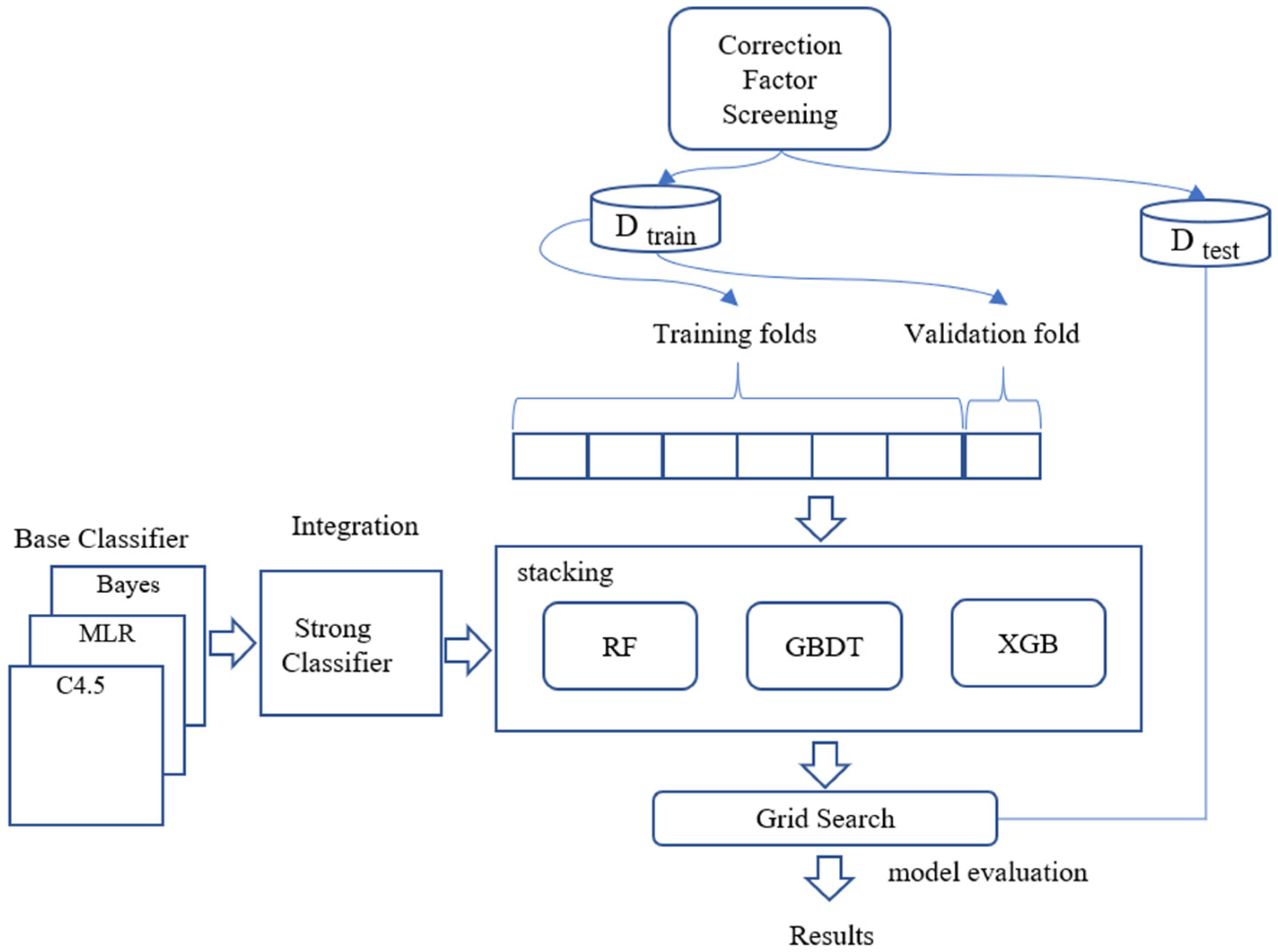
4. Ensemble Learning Correction Model
4.1. Base Classifier
4.2. Correction Factor Screening
4.3. Grid Search Data
4.4. Optimizing Model
5. Results and Evaluation
5.1. Experimental Environment
5.2. Dataset
- (1)
- The actual elements of the reporting time: PM2.5 concentration, PM10 concentration, O3 concentration, air pressure, temperature, relative humidity, 10-m wind direction, 10-m wind speed, visibility, precipitation, 3-h pressure change, 24-h pressure change, 24-h temperature change, inversion, mixed layer height, 850 hPa temperature, 925 hPa wind speed.
- (2)
- The actual elements of the revised time: PM2.5 concentration, PM10 concentration, O3 concentration.
- (3)
- The forecast elements of the correction time: PM2.5 concentration, PM10 concentration, O3 concentration, air pressure, temperature, relative humidity, 10 m wind direction, 10 m wind speed, visibility, precipitation, 3 h variable pressure, 24 h variable pressure, 24 h variable temperature, temperature inversion, mixed layer height, 850 hPa temperature, 925 hPa wind speed.
5.3. Data Pre-Processing
- (1)
- The ensemble learning correction model for missing observation data in the data set uses mean filling, taking the upper and lower observations for mean filling, such as the data unit with a value of 999,999 in the dataset.
- (2)
- Aiming at the data unit with the wind direction observation value of 999,017 in the dataset, its true meaning is the static wind state, and the ensemble learning correction model deletes its data.
5.4. Evaluating Indicator
5.5. Comparative Experiment Settings
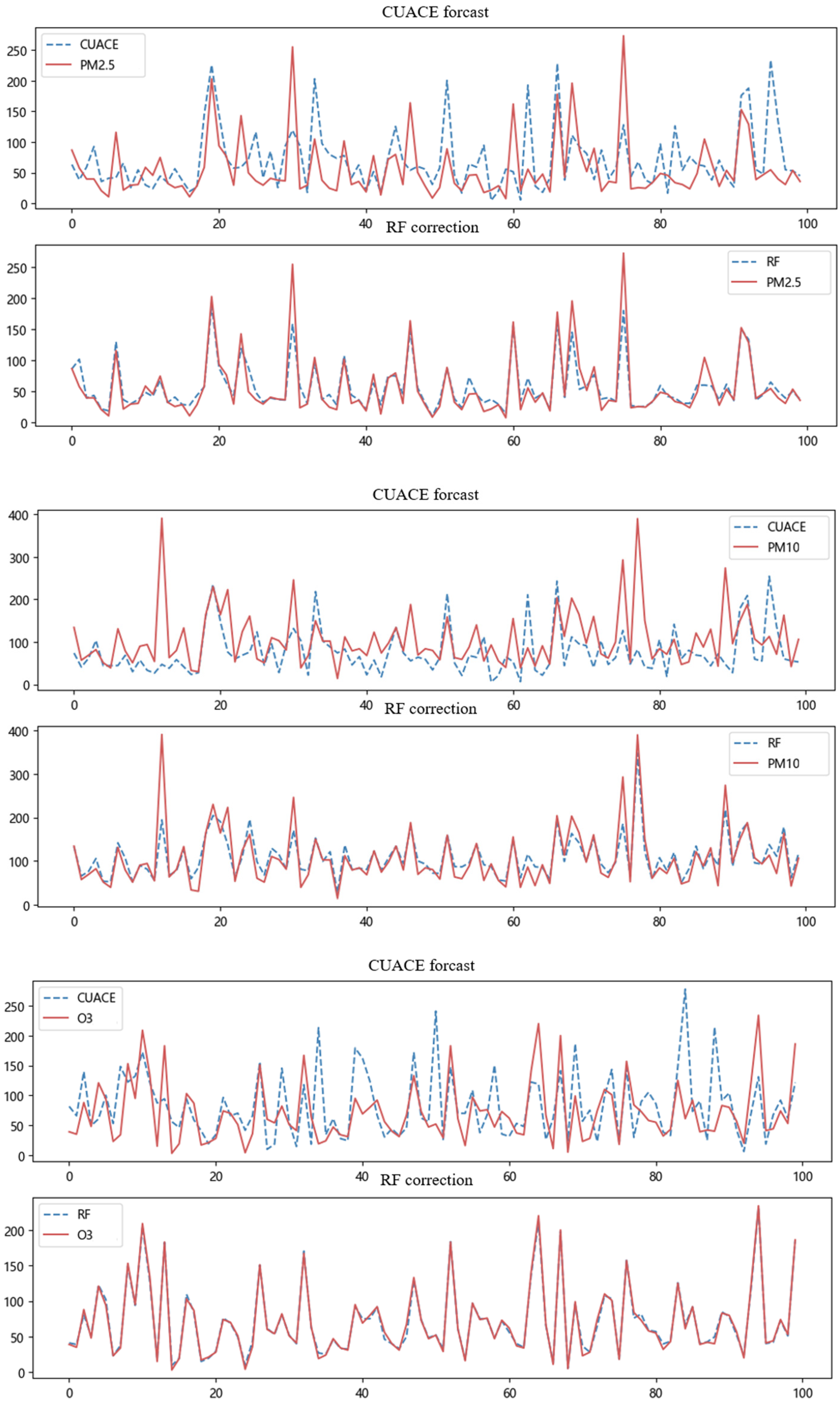
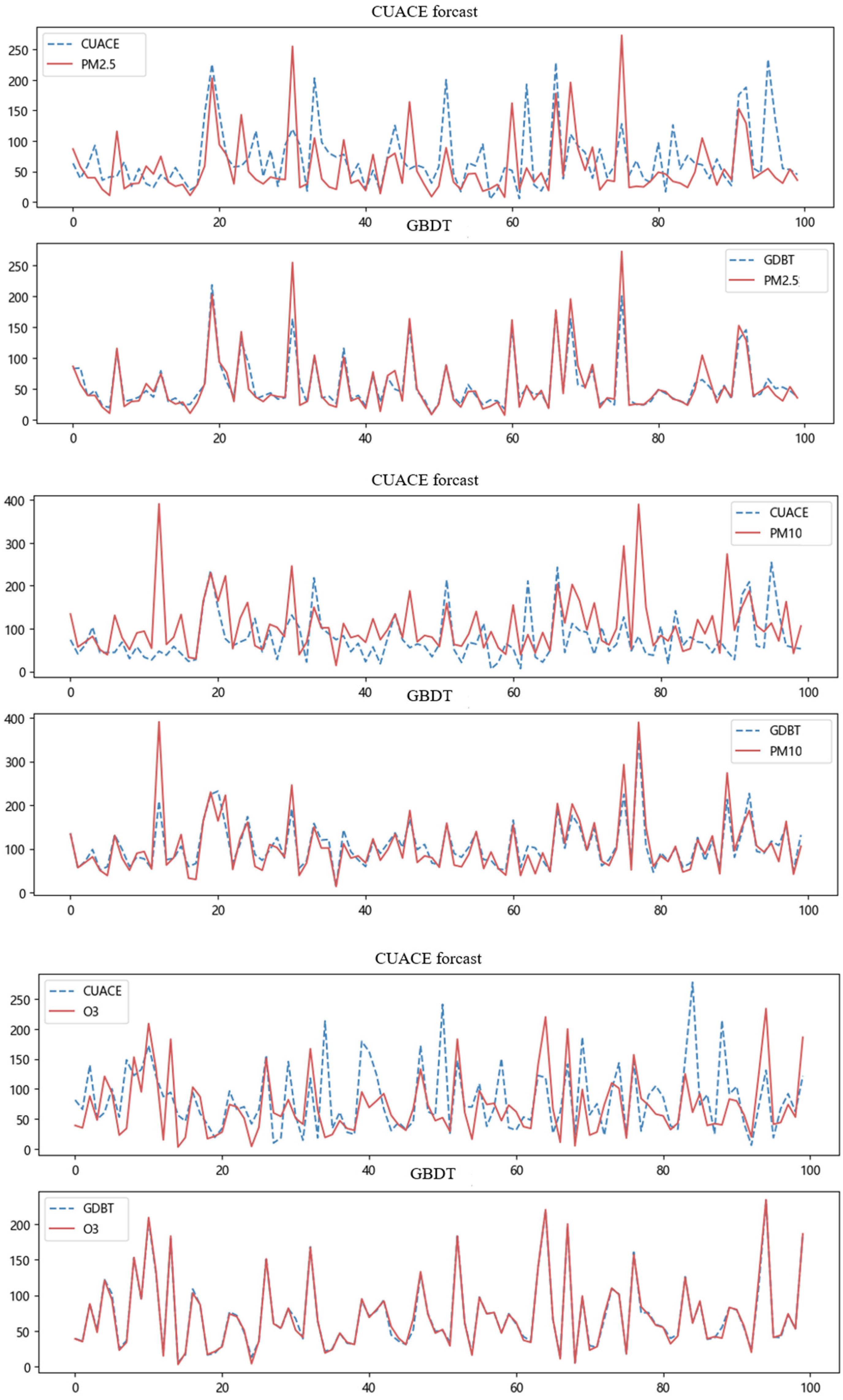
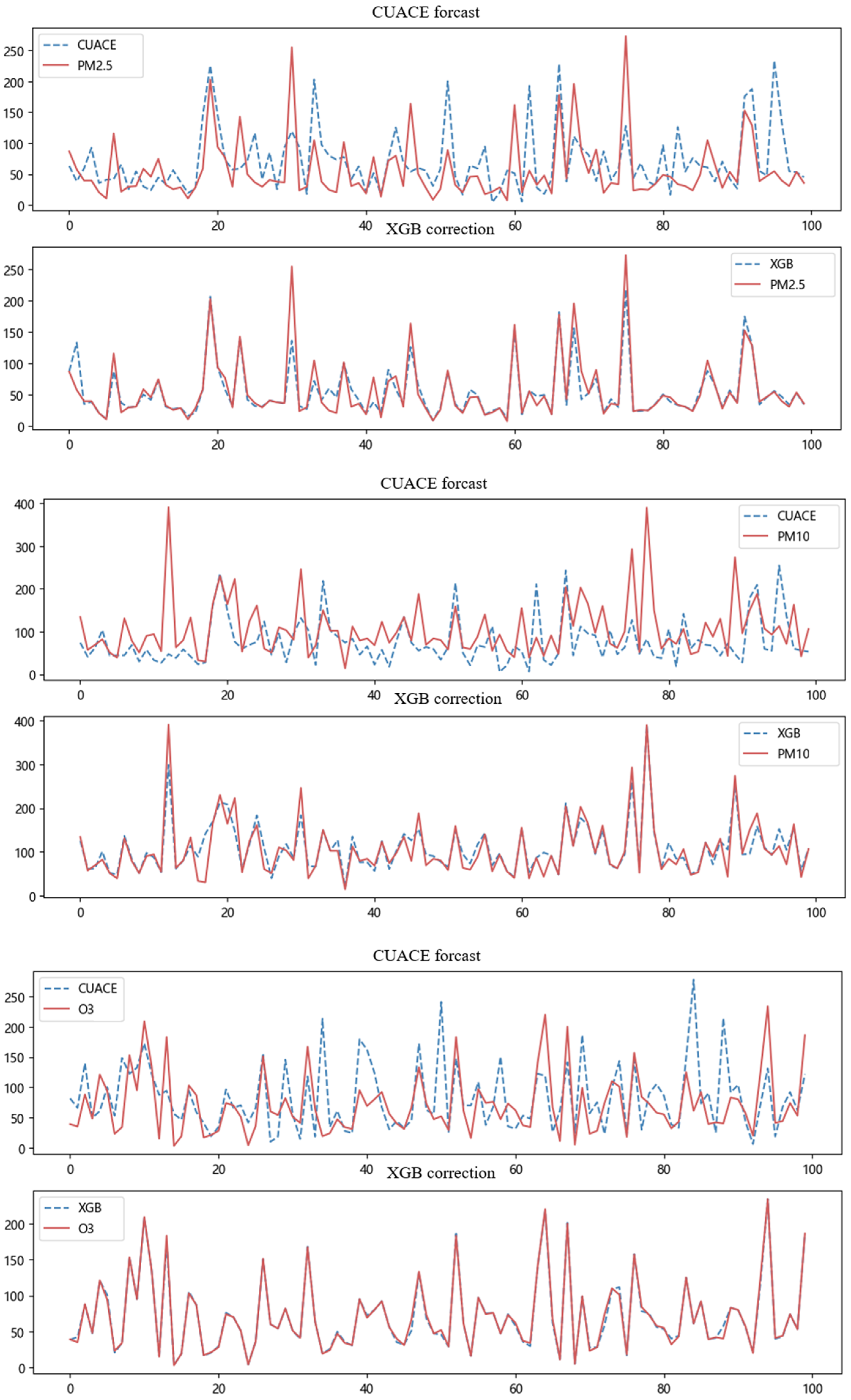
5.6. Experimental Result Analysis
6. Conclusions
Author Contributions
Funding
Conflicts of Interest
Appendix A

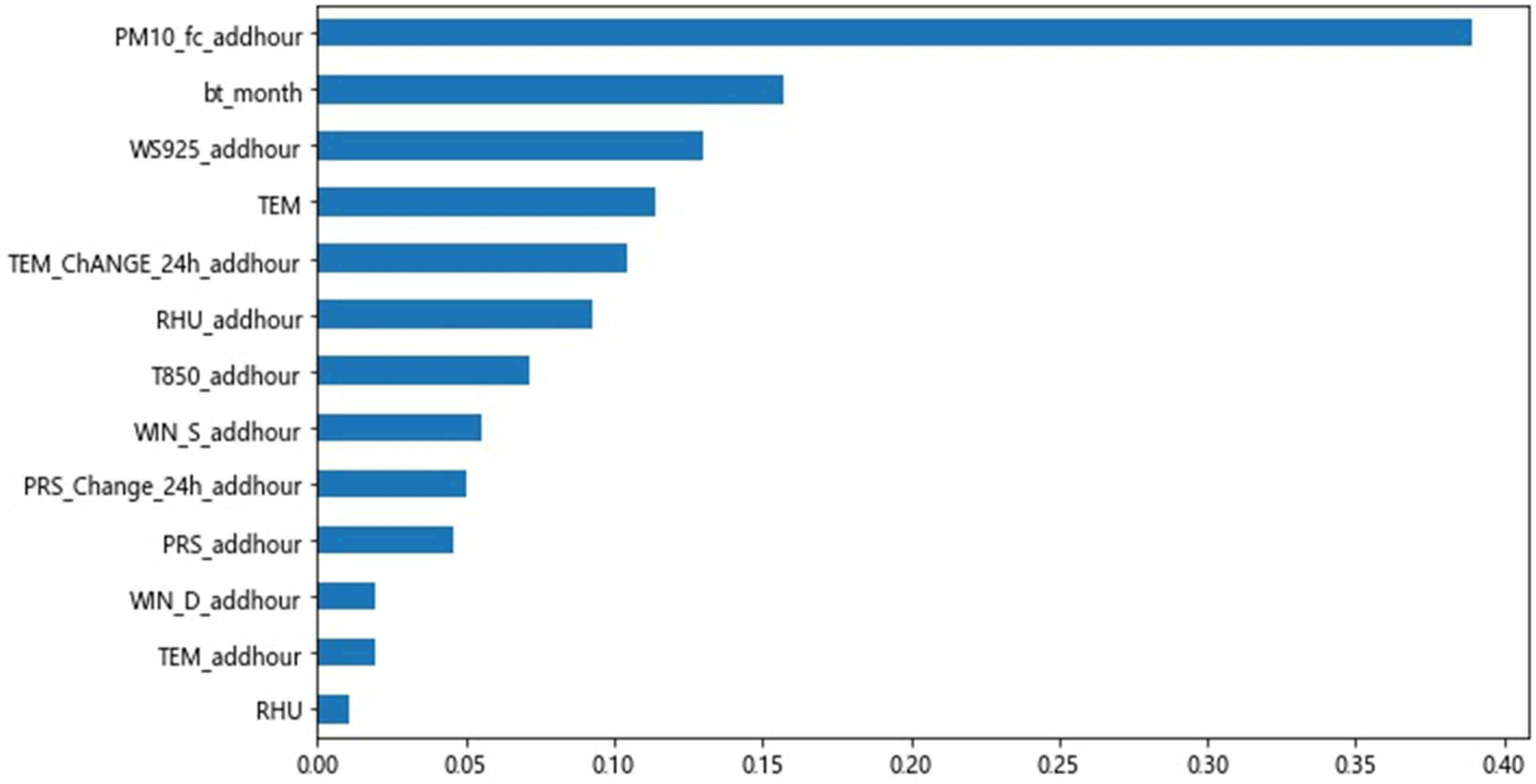
| Sort | PM2.5 | PM10 | O3 | |||
|---|---|---|---|---|---|---|
| Factor | Ratio | Factor | Ratio | Factor | Ratio | |
| 1 | VIS_fc | 0.6321 | VIS_fc | 0.3792 | TEM_fc | 0.6078 |
| 2 | RHU_fc | 0.1235 | RHU_fc | 0.2551 | MixHeight | 0.1935 |
| 3 | T850_fc | 0.0818 | TEM_24h | 0.0640 | RHU_fc | 0.0581 |
| 4 | T850 | 0.0552 | MixHeight | 0.0441 | WIN_S_fc | 0.0351 |
| 5 | T850_fc | 0.0407 | bt_month | 0.0416 | bt_month | 0.0263 |
| 6 | TEM | 0.0153 | T850 | 0.0407 | VIS_fc | 0.0194 |
| 7 | WIN_S_fc | 0.0103 | WIN_S_fc | 0.0362 | O3_fc | 0.0160 |
| 8 | bt_month | 0.0099 | PRE_fc | 0.0303 | T850_fc | 0.0123 |
| 9 | TEM_fc | 0.0043 | T850_fc | 0.0302 | PRS_fc | 0.0076 |
| 10 | PRE_fc | 0.0039 | PM10_fc | 0.0273 | WS925_fc | 0.0062 |
References
- Jiang, Y.; Wu, X.-J.; Guan, Y.-J. Effect of ambient air pollutants and meteorological variables on COVID-19 incidence. Infect. Control. Hosp. Epidemiol. 2020, 41, 1011–1015. [Google Scholar] [CrossRef] [PubMed]
- Wardah, T.; Kamil, A.; Hamid, A.S.; Maisarah, W. Statistical verification of numerical weather prediction models for quantitative precipitation forecast. In Proceedings of the 2011 IEEE Colloquium on Humanities, Science and Engineering (CHUSER), Penang, Malaysia, 5–6 December 2011; pp. 88–92. [Google Scholar]
- Wang, Y.F.; Ma, Y.J.; Quan, W.J.; Li, R.P. Research progress on application of air quality numerical forecast model in Northeast China. J. Meteorol. Environ. 2020, 36, 130–136. [Google Scholar]
- Gong, S.L.; Zhang, X.Y. CUACE/Dust-an integrated system of observation and modeling systems for operational dust forecasting in Asia. Atmos. Chem. Phys. 2007, 7, 1061–1067. [Google Scholar] [CrossRef]
- Hólm, E.V.; Lang, S.T.; Fisher, M.; Kral, T.; Bonavita, M. Distributed Observations in Meteorological Ensemble Data Assimilation and Forecasting. In Proceedings of the 2018 21st International Conference on Information Fusion (FUSION), Cambridge, UK, 10–13 July 2018; pp. 92–99. [Google Scholar]
- Yang, G.Y.; Shi, C.E.; Deng, X.L.; Zhai, J.; Huo, Y.F.; Yu, C.X.; Zhao, Q. Application of multi-model ensemble method in PM2.5 forecasting in Anhui Province. J. Environ. Sci. 2021, 41, 1–11. [Google Scholar]
- Du, J. Status and Prospects of Ensemble Forecast. Appl. Meteorol. 2002, 13, 16–28. [Google Scholar]
- Xu, J.W.; Yang, Y. Integrated Learning Methods: A Review. J. Yunnan Univ. (Nat. Sci. Ed.) 2018, 40, 1082–1092. [Google Scholar]
- Pedregosa, F.; Varoquaux, G.; Gramfort, A.; Michel, V.; Thirion, B.; Grisel, O.; Blondel, M.; Prettenhofer, P.; Weiss, R.; Dubourg, V.; et al. Scikit-learn: Machine Learning in Python. J. Mach. Learn. Res. 2012, 12, 2825–2830. [Google Scholar]
- Huang, F.L.; Xie, G.Q.; Xiao, R.L. Research on Ensemble Learning. In Proceedings of the International Conference on Artificial Intelligence and Computational Intelligence, Shanghai, China, 7–8 November 2009; pp. 249–252. [Google Scholar]
- Yang, Y.L.; Wang, J.Y.; Zhao, W. The effect of CUACE model on heavy pollution weather forecast in Yinchuan. J. Ningxia Univ. (Nat. Sci. Ed.) 2022, 43, 215–219+224. [Google Scholar]
- Krichen, M.; Mihoub, A.; Alzahrani, M.Y.; Adoni, W.Y.H.; Nahhal, T. Are Formal Methods Applicable to Machine Learning And Artificial Intelligence? In Proceedings of the 2022 2nd International Conference of Smart Systems and Emerging Technologies (SMARTTECH), Riyadh, Saudi Arabia, 9–11 May 2022; pp. 48–53. [Google Scholar]
- Perales-Gonzalez, C.; Fernandez-Navarro, F.; Carbonero-Ruz, M.; Perez-Rodriguez, J. Global Negative Correlation Learning: A Unified Framework for Global Optimization of Ensemble Models. In IEEE Transactions on Neural Networks and Learning Systems; IEEE: Piscatvie, NJ, USA, 2022; p. 99. [Google Scholar]
- Fan, X.; Feng, Z.; Yang, X.; Xu, T.; Tian, J.; Lv, N. Haze weather recognition based on multiple features and Random Forest. In Proceedings of the International Conference on Security, Pattern Analysis, and Cybernetics (SPAC), Jinan, China, 14–17 December 2018; pp. 485–488. [Google Scholar]
- Liu, S.; Cui, Y.; Ma, Y.; Liu, P. Short-term Load Forecasting Based on GBDT Combinatorial Optimization. In Proceedings of the 2018 2nd IEEE Conference on Energy Internet and Energy System Integration (EI2), Beijing, China, 20–22 October 2018; pp. 1–5. [Google Scholar]
- Li, S.T.; Wang, X.R. Application of XGBoost model in prediction of novel coronavirus. J. Chin. Mini-Micro Comput. Syst. 2021, 42, 2465–2472. [Google Scholar]
- Cao, Y.; Wang, B.; Zhao, W.; Zhang, X.; Wang, H. Research on Searching Algorithms for Unstructured Grid Remapping Based on KD Tree. In Proceedings of the 2020 IEEE 3rd International Conference on Computer and Communication Engineering Technology (CCET), Beijing, China, 14–16 August 2020; pp. 29–33. [Google Scholar]
- He, S.; Wu, P.; Yun, P.; Li, X.; Li, J. An EM algorithm for target tracking with an unknow correlation coefficient of measurement noise. Meas. Sci. Technol. 2022, 33, 045110. [Google Scholar] [CrossRef]
- Lv, M.Y.; Cheng, X.H.; Zhang, H.D.; Diao, Z.G.; Xie, C.; Liu, C.; Jiang, Q. Research on the improved method of pollutant forecast bias correction of CUACE model based on adaptive partial least squares regression. J. Environ. Sci. 2018, 38, 2735–2745. [Google Scholar]
- Chen, L.; Yu, K.A.; Qin, B.B.; Li, Y.Y.; Fan, K.F.; Li, Q.B. Evaluation and correction analysis of air quality forecast in Ningbo based on CUACE model. Technol. Bull. 2022, 38, 26–31. [Google Scholar]
- He, J.M.; Liu, K.; Wang, Y.H.; Zhang, P.Y. Verification and correction of CUACE model in urban air quality forecast in Lanzhou. Drought Meteorol. 2017, 35, 495–501. [Google Scholar]
- Zhang, B.; Lv, B.L.; Wang, X.L.; Zhang, W.X.; Hu, Y.T. Using Ensemble Deep Learning to Correct Numerical Prediction Results of Air Quality—A Case Study of WuChangshi Urban Agglomeration in Xinjiang. J. Peking Univ. (Nat. Sci. Ed.) 2020, 56, 931–938. [Google Scholar]
- Sun, Q.D.; Jiao, R.L.; Xia, J.J.; Yan, Z.W.; Li, H.C.; Sun, J.H.; Wang, L.Z.; Liang, Z.M. Research on wind speed correction of numerical weather prediction based on machine learning. Meteorology 2019, 45, 426–436. [Google Scholar]
- Chen, T.Q.; Guestrin, C. XGBoost: A Scalable Tree Boosting System. IEICE Transactions on Fundamentals of Electronics, Communications and Computer Sciences (CoRR). arXiv 2016, arXiv:1603.02754. [Google Scholar]
- Xiao, Y. Research and application of air quality numerical forecast correction method based on multi-machine learning algorithm coupling. Environ. Sci. Res. 2022, 35, 2693–2701. [Google Scholar]


| Ref. No | Author | Method/Framework | Discussion |
|---|---|---|---|
| 1 | Cheng et al. (2018) [19] | The adapting partial least square regression technique (APLSR) | The real-time dynamic correction of PM2.5 concentration predicted by GRAPES-GUACE model is carried out by introducing the measured concentration and meteorological conditions of PM2.5 and considering the influence of meteorological conditions in different seasons and regions. |
| 2 | Chen et al. (2022) [20] | The decaying averaging method and The rolling bias correction method. | After correcting the daily AQI forecast value of the CUACE model by using the decreasing average method and the rolling deviation correction method, the standard error, average deviation, and normalized deviation are all significantly reduced, and the correction effect is remarkable. |
| 3 | He et al. (2017) [21] | The error rolling linear regression correction method. | After analyzing the absolute errors of the corrected PM10, PM2.5 and NO2 pollutant concentrations, it was found that the concentration values were all significantly smaller, and the PM10 concentration was the most obvious. Therefore, after adding a certain value to the corrected results, it was found that the correct rate can be increased to more than 66%. |
| 4 | Zhang et al. (2020) [22] | An ensemble deep learning model | This paper proposes a post-correction method based on ensemble deep learning to correct the PM2.5 concentration forecast results of the original CMAQ model and improve the spatial resolution of the CMAQ forecast. |
| 5 | Sun et al. (2019) [23] | Based on LASSO regression, random forest and deep learning model | The correction effects of the three machine learning algorithms are better than those of the MOS method, which shows the potential of machine learning methods in improving local accurate weather forecasts. |
| Setting | Loss Function | |
|---|---|---|
| Regression | ||
| Huber | ||
| Classification | Deviance |
| Element | Max_Depth | N_Estimators | Best_Score |
|---|---|---|---|
| PM2.5 | 40 | 700 | 0.8 |
| PM10 | 25 | 900 | 0.81 |
| O3 | 35 | 1100 | 0.97 |
| Element | Max_Depth | N_Estimators | Best_Score |
|---|---|---|---|
| PM2.5 | 5 | 900 | 0.88 |
| PM10 | 5 | 900 | 0.86 |
| O3 | 8 | 800 | 0.98 |
| Element | N_Estimators | Best_Score |
|---|---|---|
| PM2.5 | 300 | 0.9 |
| PM10 | 500 | 0.88 |
| O3 | 500 | 0.98 |
| Experimental Environment | Configuration |
|---|---|
| Operating System | Win10 |
| CPU | Intel(R) Core (TM)i7-11800H |
| GPU | NVIDIA RTX3060 8 GB |
| Memory | 16.0 GB |
| Programming language | Python3.6 |
| Air Pollutants | Model | Evaluating Indicator | ||
|---|---|---|---|---|
| RMSE | ||||
| PM2.5 | ET-BPNN model | 0.73 | 18.23 | 13.31 |
| Ensemble learning correction model | 0.80 | 17.43 | 9.09 | |
| PM10 | ET-BPNN model | 0.63 | 26.34 | 18.82 |
| Ensemble learning correction model | 0.63 | 30.51 | 17.71 | |
| O3 | ET-BPNN model | 0.81 | 29.16 | 3.52 |
| Ensemble learning correction model | 0.99 | 5.58 | 1.59 | |
| Types of Pollutants | CUACE | RF | GBDT | XGB |
|---|---|---|---|---|
| PM2.5 | 35.46 | 12.13 | 9.95 | 9.09 |
| PM10 | 51.09 | 20.33 | 19.7 | 17.71 |
| 03 | 41 | 17.71 | 1.59 | 2.19 |
| Types of Pollutants | CUACE | RF | GBDT | XGB |
|---|---|---|---|---|
| PM2.5 | 50.73 | 20.79 | 24.76 | 17.43 |
| PM10 | 75.54 | 31.85 | 45.93 | 30.51 |
| 03 | 57.55 | 5.58 | 7.49 | 7.49 |
| Types of Pollutants | CUACE | RF | GBDT | XGB |
|---|---|---|---|---|
| PM2.5 | 0.11 | 0.80 | 0.80 | 0.89 |
| PM10 | −0.81 | 0.63 | 0.56 | 0.74 |
| 03 | −0.04 | 0.99 | 0.98 | 0.99 |
Disclaimer/Publisher’s Note: The statements, opinions and data contained in all publications are solely those of the individual author(s) and contributor(s) and not of MDPI and/or the editor(s). MDPI and/or the editor(s) disclaim responsibility for any injury to people or property resulting from any ideas, methods, instructions or products referred to in the content. |
© 2023 by the authors. Licensee MDPI, Basel, Switzerland. This article is an open access article distributed under the terms and conditions of the Creative Commons Attribution (CC BY) license (https://creativecommons.org/licenses/by/4.0/).
Share and Cite
Ma, J.; Ma, X.; Yang, C.; Xie, L.; Zhang, W.; Li, X. An Air Pollutant Forecast Correction Model Based on Ensemble Learning Algorithm. Electronics 2023, 12, 1463. https://doi.org/10.3390/electronics12061463
Ma J, Ma X, Yang C, Xie L, Zhang W, Li X. An Air Pollutant Forecast Correction Model Based on Ensemble Learning Algorithm. Electronics. 2023; 12(6):1463. https://doi.org/10.3390/electronics12061463
Chicago/Turabian StyleMa, Jianhong, Xiaoyan Ma, Cong Yang, Lipeng Xie, Weixing Zhang, and Xuexiang Li. 2023. "An Air Pollutant Forecast Correction Model Based on Ensemble Learning Algorithm" Electronics 12, no. 6: 1463. https://doi.org/10.3390/electronics12061463
APA StyleMa, J., Ma, X., Yang, C., Xie, L., Zhang, W., & Li, X. (2023). An Air Pollutant Forecast Correction Model Based on Ensemble Learning Algorithm. Electronics, 12(6), 1463. https://doi.org/10.3390/electronics12061463