1. Introduction
The terms Artificial Intelligence (AI), Machine Learning (ML), and Deep Learning (DL) are frequently used interchangeably. From a holistic perspective, DL is a subcategory of ML which, in turn, is a subdivision of AI. Artificial intelligence is a far-reaching branch of computer science in which a range of tools and techniques are used to make machines (namely computers and robots) more intelligent and consequently more effective and efficient. Computational methods of ML such as Neural Networks (NNs), support vector machines, and decision trees are employed to find relevant patterns within a dataset. DL methods represent more sophisticated extensions of classical ML techniques and are generally superior to them. There are various DL algorithms such as Convolutional Neural Networks (CNNs), deep auto-encoders, and generative adversarial networks.
ML and DL models have been introduced in various fields [
1,
2,
3,
4,
5,
6,
7,
8] to make decisions using available data and domain knowledge. It is crucial to consider both accuracy and reliability when evaluating such models. These models are typically assessed based on their accuracy using statistical error metrics such as: (i) for regression: the coefficient of determination (R
2), Mean Squared Error (MSE), and relative error, and (ii) for classification: precision, F1 score, and confusion matrix.
In terms of reliability, ML and DL deal with two main types of uncertainty: (i) aleatoric uncertainty (also called irreducible uncertainty/data uncertainty/inherent randomness) and (ii) epistemic uncertainty (also called knowledge uncertainty/subjective uncertainty) [
9]. Aleatoric uncertainty arises from an inherent property of the data and cannot be reduced even with a higher volume of samples. The data used to develop a model can be sourced from experimental measurements, collected from other resources, or produced via simulation/programming. This data always contains noise, which refers to the data distribution and errors made while measuring, collecting, or generating data. A related problem is incomplete coverage of the domain. That is why most models are constructed based on a limited range of data and cannot be generalized. Epistemic uncertainty is a property of a model caused by factors such as the selection of very simple or complex structures, the stochastic nature of optimization algorithms, or the type of statistical error metrics. This uncertainty is reducible by feeding enough training samples into the model.
Uncertainty Quantification (UQ) techniques are beneficial to limit the effect of uncertainties on decision-making processes. According to [
9], there are three main types of UQ: (i) Bayesian methods such as Monte Carlo (MC) dropout, Markov Chain Monte Carlo, variational inference, Bayesian active learning, Bayes by backprop, variational autoencoders, Laplacian approximations, and UQ in reinforcement learning like Bayes-adaptive Markov decision process, (ii) ensemble techniques such as deep ensemble, deep ensemble Bayesian/Bayesian deep ensemble, and uncertainty in Dirichlet deep networks like information-aware Dirichlet networks, and (iii) other methods such as deep Gaussian Process (GP) and UQ in the traditional ML domain using ensemble techniques like support vector machine with Gaussian sample uncertainty.
Typically, researchers tend to apply their techniques or methods to existing datasets. Even when using new data, it may still face limitations such as restricted sample size or low dimensionality. Moreover, while both classification and regression algorithms are supervised learning techniques, previous studies on DL have mostly focused on classification, and regression has received much less attention. Additionally, despite much research into the accuracy of DL models, their reliability analysis remains inadequate. Finally, MC dropout is a computationally efficient method that uses dropout as a regularization term to estimate uncertainty. Putting these points together, the main contribution of this paper is to demonstrate the potential of using MC dropout in skip connection-based CNN models based on big data.
A high-dimensional regression problem from the domain of petroleum engineering is included as a case study because subsurface flow problems usually involve some degree of uncertainty due to the lack of data with which models are constructed. Moreover, despite extensive efforts towards renewable energy, the oil/gas sector still supplies a significant proportion of global energy consumption, so this research has real-world applications.
The rest of this paper is arranged as follows.
Section 2 provides an overview of MC dropout and references a number of relevant publications. In
Section 3, the mixed Generalized Multiscale Finite Element Method (GMsFEM) is briefly explained as a case study.
Section 4 presents the characteristics of the skip connection-based CNN models used along with MC dropout. The results are given in
Section 5.
Section 6 provides some discussion and the limitation of the research. The conclusions and future study are given in
Section 7.
2. MC Dropout and Its Related Work
Standard deterministic deep NNs operate on a one-input-one-output basis. Unlike single-point predictions of such models, Bayesian methods such as Bayesian Neural Networks (BNNs) and (GPs) give predictive distributions. The weights of BNNs are incorporated with prior distributions, whereas GPs introduce priors over functions. A drawback of BNNs and GPs is the computational cost, which becomes prohibitive given a very large network, as in the case of deep networks. Bayesian neural networks need to get the posterior distribution across the network’s parameters, in which all possible events are obtained at the output. Gaussian processes require us to sample prior functions from multivariate Gaussian distribution, wherein the dimension of Gaussian distribution increases proportionally with the number of training points involving the whole dataset during predictions.
A computationally more efficient method called MC dropout has been recently developed [
10]. A NN with any depth and non-linearities accompanying dropout before weight layers might be interpreted as a Bayesian approximation of the probabilistic deep GP. Additionally, the dropout objective minimizes Kullback-Leibler (KL) divergence between an approximate distribution and the posterior of a deep GP.
Dropout basically serves as a regularization technique within the training process to reduce over-fitting in NNs. For the testing samples, the dropout is not applied, but weights are adjusted, e.g., multiplied by `1 − dropout ratio’. With regards to MC dropout, the dropout is applied at both training and test time. So, the prediction is no longer deterministic at test time.
Given that
is an output of a NN model with hidden layers
L. Also,
represents the NN’s weight matrices, and
is the observed output corresponding to input
. By defining
and
as the input and output sets, the predictive distribution is expressed as:
here,
and
are the NN model’s likelihood and the posterior over the weights.
The predictive mean and variance are used in the predictive distribution to estimate uncertainty. The posterior distribution is, however, analytically intractable. As a replacement, an approximation of variational distribution
can be obtained from the GP such that it is as close to
as possible, in which the optimization process happens through the minimization of the KL divergence between the preceded distributions as shown below:
With variational inference, the predictive distribution can be described as follows:
According to [
10],
is selected to be the matrices distribution whose columns are randomly set to zero given a Bernoulli distribution, specified as:
where
for
and
with
as the dimension of matrix
. Also,
represents the probability of dropout and
is a matrix of variational parameters. Therefore, drawing
T sets of vectors of samples from Bernoulli distribution gives
, and consequently, the predictive mean will be:
where
is the output obtained by the given NN for input
, and
is the predictive mean of MC dropout, equivalent to doing
T stochastic forward passes over the network during the testing process with dropout and then averaging the results. It is useful to view this method as an ensemble of approximated functions with shared parameters, which approximates the probabilistic Bayesian method known as deep GP. In this method, there are several outputs (considered 30, 50, 100, and 200 in this research) for a given input. Subsequently, uncertainty could be examined in terms of factors such as variance, entropy, and mutual information.
In the following, four examples are given to show the application of MC dropout in modeling subsurface fluid flow. The researchers in [
11] investigated the uncertainty involved in ML seismic image segmentation models. Salt body detection was considered as an example. They used MC dropout and concluded the developed models were reliable.
The researchers in [
12] used the dropout method for a classification problem to quantify the fault model uncertainty of a reservoir in the Netherlands. The networks were trained with dropout ratios of 0.25 and 0.5. The researchers concluded that the model variance increased by increasing the dropout ratio. Also, they suggested training with more data is needed.
The MC dropout approach and a bootstrap aggregating method were used to quantify uncertainties of CO
2 saturation based on seismic data in [
13]. The researchers carried out DL inversion experiments using noise-free and noisy data. The results showed that the model can estimate 2D distributions of CO
2 moderately well, and UQ can be done in real-time.
A semi-supervised learning workflow was used to effectively integrate seismic data and well logs and simultaneously predict subsurface characteristics in [
14]. It had three distinct benefits: (i) using 3D seismic patterns for developing an optimal nonlinear mapping function with 1D logs, (ii) being capable of automatically filling the gap of vertical resolution between seismic and well logs, and (iii) having an MC dropout-based epistemic uncertainty analysis. The results of the two examples showed reliable seismic and well integration, and robust estimation of properties like density and porosity obtained by this procedure.
3. Case Study
Fluid flow in petroleum reservoirs is typically governed by: (i) the equation of mass conservation, (ii) momentum law (Darcy’s law), (iii) energy equation, (iv) fluid phase behavior equations (also known as equations of state) and certain rock property relationships (such as compressibility) [
15]. To solve this system of equations, it is necessary to specify boundaries and initial conditions. Analytical (exact) solutions can be determined for relatively simple reservoirs (i.e., by making several assumptions). An alternative is to apply numerical (approximate) solutions, such as the finite difference method, Finite Element Method (FEM), finite volume method, spectral method, and meshless method.
A mixed GMsFEM framework, as a numerical method, has recently been proposed for a single-phase fluid in 2D heterogeneous (matrix composition and fracture distribution) porous media [
16]. The model approximates reservoir pressure in multiscale space. It does so by applying several multiscale basis functions to a single coarse grid of the reservoir volume. The fluid velocity is directly estimated across a fine grid space. Generally, the number of Partial Differential Equations (PDEs) requiring solutions to enable multiscale basis functions to be derived is dependent on the number of local cell and local eigenvalue problems involved, which necessitates a substantial overhead. Therefore, it is reasonable to replace PDE solvers with ML/DL approaches, given their exceptional abilities and general acceptance in recent years. Readers are referred to [
16] for additional information, especially what the original flow problem is and how the mixed GMsFEM works.
For the configuration defined in this paper, the computational domain was set to be
(
Figure 1). The fine grid system adopted involves a uniform
mesh. On the other hand, a sparser, uniform
mesh was applied to represent the coarse grid network. This configuration consists of 1300 separate PDEs, made up of 1200 (
) PDEs addressing the local cell problems plus 100 (
) local eigenvalue problems. There were five multiscale basis functions, identified as Basis 1, 2, 3, 4, and 5 for each generated permeability field (as the only input). A range of values for the permeability of the matrix was chosen from 1 to 5 milliDarcies (mD) incrementing in steps of 1 (i.e., 1, 2, 3, 4, and 5 mD); and for the permeability of the fracture from 500 to 2000 mD incrementing in steps of 250 (i.e., 500, 750, 1000, 1250, 1500, 1750, and 2000 mD). The number of fractures was set to 1, 2, 3, …, 23, 24, and 25 (25 cases). Basis 1 is a piecewise constant, with binary values of −1 and +1. Basis 1 is defined as part of FEM, it hence requires no training for DL modeling. However, Basis 2, 3, 4, and 5 take values distributed across the range (−1, +1), and therefore require training for DL modeling.
In terms of supervised learning, our problem was mapping an input of to an output of . Because there were four different basis functions, we had four distinct mappings. In this regard, 376,250 samples were produced in the MatLab software including 306,250 examples for the training, 35,000 for the validation, and 35,000 for the testing. Due to the random generation of the permeability fields, duplicates might have been present. Consequently, the generated dataset was filtered to remove any duplicate data records. This is necessary to remove the risk of introducing bias towards specific model configurations in the DL analysis. For our data, 1739 training, 579 validation, and 6121 testing samples were kept out. This reduced the training, validation, and testing samples to 304,511, 34,421, and 28,879, respectively.
4. Skip Connection-Based CNN Model Architecture
Depending on the way in which an algorithm learns from data sets, DL (and also ML) algorithms fall into four categories: (i) supervised, (ii) unsupervised, (iii) semi-supervised, and (iv) reinforcement. Our problem is a supervised learning task. There are several approaches that can be adopted in this category such as recurrent neural networks and CNNs. Recurrent neural networks are often applied to process video, sound, and text data. On the other side, CNNs are particularly designed for problems involving 2D arrays like the regression case study in this research, where an input of is mapped to an output of . The format defined for the permeability field was as a () vector, subsequently adjusted to be expressed as a 2D tensor (), in which, coarse grid units = 100 and each coarse grid contains 9 fine grids. Each row in the array, therefore, represents a coarse grid. Such a configuration enables the use of 2D CNN kernels. Furthermore, there was a logical and convincing mathematical procedure behind convolutional filters. Convolutional neural networks also automatically and adaptively learn the spatial hierarchies of features. Lastly, it can reduce the number of parameters without sacrificing model quality. With regards to the output, it was necessary to maintain the five basis functions as vectors, so that they could be evaluated in the Fully Connected (FC) layers (dense layers) forming the final section of the CNN network.
A classic CNN model is normally composed of alternate convolutional and pooling layers, followed by one or more FC layers at the end. In some situations, it is sensible to replace an FC layer with a global average pooling layer. The convolutional and pooling layers perform feature extraction, while the FC layers map the extracted features into an output layer.
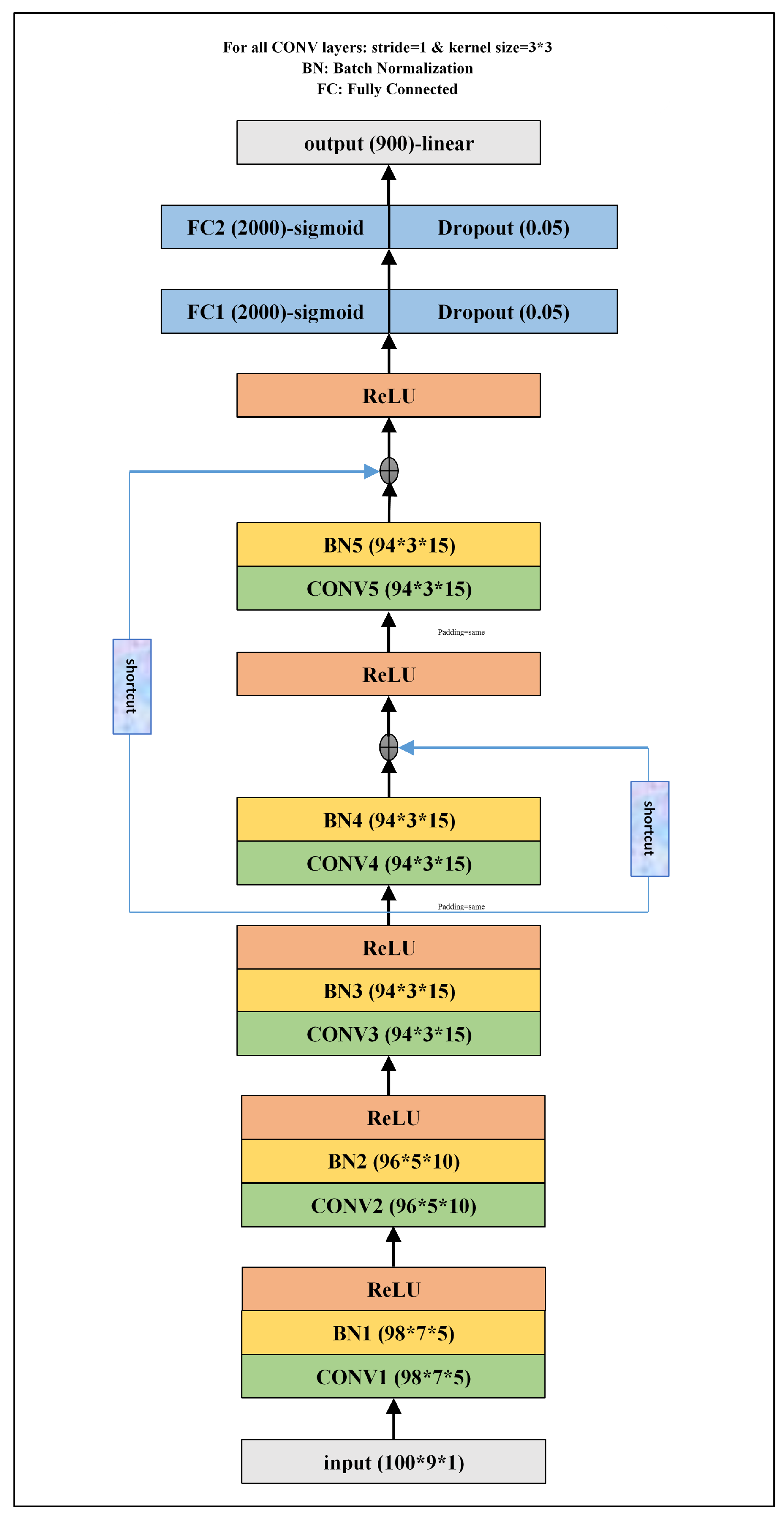
Distinct CNN model configurations, involving various combinations of convolutional, pooling, FC, Batch Normalization (BN), regularization, and dropout filtering were tested separately on each basis function requiring training (Basis 2, 3, 4, and 5). A similar optimal CNN configuration was obtained for each of those four basis functions (
Figure 2). It consists of five convolutional layers and two FC layers, but does not include any pooling layers. Each convolutional layer is followed by a single BN layer of the same dimensions. Typically, neural network models can apply higher learning rates and converge more quickly when the input to each layer is normalized; hence the value of adding the BN layers. The two FC layers contain 2000 neurons with a dropout rate of 0.05.
The gradient of the loss function might quickly approach zero when a deep NN back propagates the gradient from the final layers to earlier layers close to the input layer. This refers to the ’vanishing gradient problem’, which makes the earlier layers not benefit from additional training. Using the skip connection (shortcut) strategy, which enables the gradient to be directly back-propagated to earlier layers of a network, is one of the most effective ways to tackle this problem. After testing different cases, we found out it would be better to add simultaneously two shortcut schemes to the main CNN structure: (i) from the middle to the last layer and (ii) from the middle to the second-to-last layer.
The model, treated as a Bayesian approach, produces a different output each time called with the same input. This is because each time a new set of weights is sampled from the distributions to develop the network and produce an output. After examining various cases, we discovered that 30 outputs are the ideal case for a given input, representing the most efficient and effective solution. The models employ the activation function of ‘Rectified Linear Unit (ReLU)’ for the convolutional layers, ‘sigmoid’ for the FC layers, and ‘linear’ for the output.
5. Evaluation
To understand the role of MC dropout in the developed CNN models based on accuracy, two statistical error metrics of R
2 and MSE are included:
where
,
, and
are the actual basis function of the
i-th data point, the average of actual basis function for all samples, and the predicted basis function for the
i-th data point, respectively. Also,
N is the number of data points. As mentioned earlier, each basis function is in the form of a
tensor and R
2 of all outputs are averaged, weighted by the variances of each individual output. The R
2 value lies between
and 1 [
17]. The closer the value is to 1, the more accurate the predictions produced by the model. The error metric of MSE measures the average of squares of errors (i.e., the difference between predicted and real values). It is basically non-negative, where values closer to zero indicate more-accurate performance. The models without dropout yield promising results when evaluated on the training subset using R
2 and MSE metrics. Except for Basis 5, the R
2 of others is above 0.9. The values obtained for MSE lie within the range of 0.0075 to 0.0243. The constructed models perform suitably for the validation subset, with an R
2 of 0.7900 to 0.8811 and a MSE of 0.0128 to 0.0512. Because the validation and testing subsets were selected from a similar distribution of data, we can see almost the same results over the testing samples: an R
2 of 0.7857 to 0.8809, and MSE 0.0126 of to 0.0513.
According to
Table 1, the dropout after two FC layers enhances performance over all subsets for all multiscale basis functions. For the training subset, it has the maximum effect on the model for Basis 3 and the minimum effect for Basis 4. For basis 3, R
2 increases from 0.9327 to 0.9584, and MSE decreases from 0.0141 to 0.0113. There is an R
2 increase from 0.9283 to 0.9326 and an MSE decrease from 0.0107 to 0.0101 for Basis 4.
Adding dropout to the initial architecture has generally a marginally positive effect on the validation and testing samples. The range of R2 and MSE is 0.7919–0.8858 and 0.0120–0.0507 for validation. The R2 and MSE lie in the range of 0.7881–0.8839 and 0.0121–0.0508 for testing.
As a general result, it is evident that the use of dropout has a positive impact on the performance of the developed models across the training subset, regardless of the basis functions used. Furthermore, it also demonstrates a similar positive impact over the validation and testing subsets for Basis 3 and Basis 5. However, for Basis 2 and Basis 4, there is only a marginal difference between the performance of CNNinitial and CNNdropout models. The probable reasons for this could be attributed to the high-dimensional regression problem considered in this paper and the complexity and non-linear nature of DL models. Nonetheless, even this slight improvement in the models’ performance could help reduce overfitting and enhance generalization in the constructed CNNdropout models. Additionally, it can significantly affect the pressure distribution obtained through the basis functions.
Depending on the input/output dimensions, type (classification/regression), and approach applied to a problem, the magnitude of uncertainty can be analyzed statistically and graphically. Standard Deviation (SD) measures the dispersion of a data set relative to its average. It is the square root of the variance. The closer the value of SD is to zero, the values of data are closer to the average. A high SD indicates that the values are spread out over a broad range. Basically, the variance and SD are defined for a single-point data set (there is only one output). On the other hand, the output (basis functions) in this study is in the form of a vector. While dealing with a vector, it is necessary to calculate the variance of each element of the vector separately. Then, the obtained variances are averaged to reach the total variance. Finally, the SD is obtained as the square root of the variance for each case. Standard CNNs (without dropout) give only one output for a given input. That is why the SD is not defined for such models (it is always zero).
According to
Table 2, the SD values lie within 0.0181–0.158, 0.0179–0.152, 0.0169–0.104, and 0.0121–0.086 for the CNN models with dropout developed for Basis 2, 3, 4, and 5 based on the training subset. For all basis functions, most samples have an SD lower than 0.05. For instance, 221,006 out of 304,511 samples for Basis 3 are in the range of 0–0.05. In general, SD exceeds 0.15 only for 547 samples. The SD obtained for Basis 4 and 5 is lower than that for Basis 2 and 3.
With regards to the validation subset, the developed models for Basis 2, 3, 4, and 5 have an SD of 0.0268–0.174, 0.0237–0.124, 0.019–0.171, and 0.012–0.097, respectively. Generally, only 27 out of 34,421 samples have an SD higher than 0.15. The model built for Basis 5 has the best performance in terms of uncertainty, with 24,276 samples with an SD of lower than 0.05 and 10,145 samples with an SD of 0.05–0.1. After that, the models developed for Basis 4 and 3 come. The model designed for Basis 2 has the worst performance because only 2577 samples have an SD of 0–0.05.
For the testing subset, the SD values lie within 0.025–0.169, 0.024–0.142, 0.020–0.113, and 0.012–0.098 for the CNN models with dropout developed for Basis 2, 3, 4, and 5. The trend is the same as the validation subset. In other words, the model for Basis 5 has the best, and the one for Basis 2 has the worst performance, respectively. Also, there is no sample with an SD higher than 0.15, except with 24 cases for Basis 2.
As mentioned earlier, the output is in the form of a
vector, which is too big to show in a graph. Additionally, basis functions in the mixed GMsFEM are defined in one coarse grid element, which includes 9 fine grids.
Figure 3 gives the 30 values obtained for each of the nine points using MC dropout for a coarse grid with the matrix permeability of 1 mD (as a representative sample). The average of 30 outputs (for each point) is considered the model’s output. The figure demonstrates that the values are close to each other (some overlap) and have a very low SD.
In order to visualize the pressure changes over the defined computational domain, three examples are illustrated for selected training (
Figure 4a), validation (
Figure 4b), and testing (
Figure 4c) subsets. The plots in the left-side columns display the permeability fields, for representative sample grids. The plots in the central columns display the pressure distribution derived by FEM (considered to be true distribution). The plots in the right-side columns display the predicted pressure distributions using the skip connection-based CNN models developed in this study. In fact, the pressure is obtained through the multiscale basis functions. Generally, there is a better match for the training sample in comparison with the validation and testing cases.
6. Discussion
In terms of accuracy, it was perceived that considering high initial sets of weights does not influence the accuracy of the models. More specifically, no meaningful improvement was observed by defining 50, 100, and 200 sets. Hence, the number of 30 sets considered here seems almost optimal given the developed models’ high accuracy and low SD for multiscale basis functions.
In a standard deterministic NN, a single prediction is obtained for a given input, with no information about the uncertainty of the used data or the model fitness. This is because only one initial set of weights/biases is used/updated in such models. The Bayesian methods can be applied to tackle this issue somewhat, taking a positive step toward the reliability of NN models. Bayesian neural networks are different from standard NNs in that their weights are assigned a probability distribution rather than a single value or point estimate. These probability distributions describe the uncertainty in weights and can be used to estimate uncertainty in predictions. In this research, we used the MC dropout only for the FC layers of the CNN structures. In other words, the dropout technique was not used regarding the convolutional layers because it negatively affected the accuracy of the models. Moreover, although multiple techniques were used to quantify the data uncertainty, we got some errors. So, it would be better to consider both uncertainty sources to construct more reliable CNN models.
In terms of UQ statistical investigation, we defined several indices for uncertainty such as entropy, Negative Log Likelihood (NLL), and SD for the statistical measures. However, the values obtained for entropy and NLL were meaningless. Therefore, it would be helpful to use more applicable statistical measures to convey the information about the uncertainty more meaningfully.
7. Conclusions
Standard deterministic deep NNs converge on a one-input-one-output basis, with no information about the uncertainty of the data or model fitness. Bayesian approaches are effective in uncertainty estimations. However, they face a high computational cost when applied to large datasets. That is why MC dropout, a computationally more efficient method, was used in this study as a positive step towards the reliability of skip connection-based CNN models based on 376,250 samples from the oil/gas domain. The SD values obtained confirm the robustness of MC dropout in terms of epistemic uncertainty, in addition to the high degree of accuracy. There are two suggestions for mitigating the limitations of the present study: (i) quantifying the aleatoric uncertainty for the developed models, and (ii) using more dropout ratios and comparing it with the ratio of 0.05 considered here.


