Fault Location Method for an Active Distribution Network Based on a Hierarchical Optimization Model and Fault Confidence Factors

Abstract

With extensive access to distributed power sources and the rising electricity load, the structure and tide of distribution networks are becoming increasingly large and complex, leading to great challenges for fault location methods. In this paper, the power coupling phenomenon of the T-section in the distribution network is studied, and a hierarchical optimization model for fault location is proposed based on the port equivalence principle, which divides the fault location into two levels—area location and section location—to reduce the fault search dimension. Then, an improved binary particle swarm optimization algorithm (IBPSO) applied to the area location is proposed to improve the convergence accuracy and speed by optimizing the convergence criterion and integrating the chaotic mapping and mutation strategies. Finally, based on the topological characteristics of the sections in the fault area, a fault candidate scenario screening method based on the fault confidence factor is proposed to realize a second dimensionality reduction in the section location link. Simulation tests show that the proposed method demonstrates a good dimensionality reduction effect for large-scale, active distribution networks; additionally, the accuracy rate is improved by 25.7% and the location speed is improved by 300 ms when compared with traditional fault location methods.

1. Introduction

1.1. Background

Following a fault in a distribution network, rapid and accurate fault location is conducive to quickly isolating the fault and restoring the power supply to the lost load. This plays an important role in improving the reliability of the power supply to the power system [1,2]. Distributed generation (DG), including solar and wind power, has the advantages of being clean and pollution-free, low-carbon, and renewable. It has been widely used in recent years [3]. With a large number of DG interconnections, the distribution network changes from a single-supply radial network to a complex, multi-source network. Additionally, the short-circuit current flows in both directions after a fault, causing the traditional fault location method of a single-supply radiation network to no longer be applicable [4]. At the same time, the expansion of the network scale, the distortion of fault information, and the dynamic switch on–switch off of DG also place positive higher requirements and challenges on the reliability and speed of fault location for active distribution networks [5].

With the development of distribution automation technology, intelligent monitoring equipment such as the feeder terminal unit (FTU) has gradually become popular [6]. The FTU, which is installed at the sectional switch, can be equipped with fault current detection components and power direction components which adjust the action threshold of the fault current detection components adaptively in accordance with the operation mode of the system [7]. After a fault in the distribution network, the FTUs identify the fault current flowing through the switch and upload the fault detection results via the communication network to the fault location decision servers, which then locate the fault based on the FTU fault information [8]. A fault location system based on FTU fault information is shown in Figure 1.

A fault location system based on FTU fault information is shown in Figure 1. The FTU installed at the intelligent switch and the decision server installed at the substation form a primary/secondary structure, and they realize information interaction through the communication network. When the distribution network is in normal operation, the decision server collects the switch status information reported by the FTU for topology identification and clarifies its jurisdiction and the connection relationship between the nodes and sections. When a fault occurs in the distribution network, the decision server collects the fault information of FTUs within its jurisdiction, calls the fault location algorithm to determine the fault location, and then issues a trip command to the relevant FTU. When the distribution network topology is changed, the FTU reports the switch status change information and the decision server reperforms a topology identification to flexibly adapt to the network topology change [9]. This method based on FTU fault information has the advantages of small data communication a, high locating efficiency, and convenient implementation [10], and it has become a hot research topic in the field of active distribution network fault location.

1.2. Literature Review

Distribution network fault location methods that are based on FTU fault information mainly include three types: the first type is the fault location method based on a matrix algorithm; the second type is the fault location method based on an intelligent optimization algorithm; and the third type is the fault location method based on a hierarchical optimization model.

(1) A fault location method for a distribution network. The basic idea of this method is to build a network description matrix based on the distribution network topology, combine the fault information reported by the FTU after the fault to build a fault discrimination matrix, and locate the fault section through a comprehensive analysis of the fault discrimination matrix [11,12]. This method has the advantages of a simple principle and fast calculation speed. However, in actual engineering, FTUs are mostly installed outdoors and work in harsh environments, and the reported fault information may be distorted; this may interfere with the formation of the matrix and cause the algorithm function to fail [13]. Although some scholars have proposed improved algorithms to improve the fault tolerance of the information [14,15], it still has a poor compatibility feature, and the fault tolerance process of the algorithm increase the fault location time greatly [16]. In addition to the expansion of the network scale, the number of FTU measurement points increases, and the probability of fault information distortion increases. Therefore, it is difficult to apply this method to solve complex active distribution network fault location problems.

(2) A fault location method based on an intelligent optimization algorithm. The basic idea of this method is to compose a solution space of all possible fault scenarios in the distribution network by the fault hypothesis and apply the optimization theory in the solution space to find the optimal solution that can provide the best explanation of the FTU fault information [17]. At present, such methods mainly include the genetic algorithm (GA) [18], binary particle swarm optimization algorithm (BPSO) [19], harmony search algorithm (HS) [20], electromagnetism-like mechanism algorithm (EIM) [21], etc. Intelligent optimization algorithms have the advantages of a high information tolerance and high generality. However, the algorithms require iterative operations, and the computational efficiency is reduced to a large extent when the solution space is expanded. In addition, the search in the solution space of the algorithm has a certain randomness which leads to a certain probability of local convergence, and it is difficult to guarantee the stability of the fault location result when the solution space is expanded [22]. In addition to the expansion of the distribution network the solution space increases, thus limiting the application of the intelligent optimization algorithm.

(3) A fault location method based on a hierarchical optimization model. The literature [23] proposes that the branch of the distribution network is externally equivalent to an area based on the equivalence principle and constructs a hierarchical optimization model of the fault location. The basic principle of this approach is to divide the fault location operation into two hierarchical levels: the first level locates the fault area, which determines the area where the fault is located based on the fault information of the port FTU measurement points; the second level locates the fault section, which further determines the feeder section where the fault occurs based on the fault information of the FTU measurement points inside the fault area. Scholars have since successively used intelligent algorithms such as the immune optimization algorithm (IA) [24], bald eagle search algorithm (BES) [25], and manta ray foraging optimization algorithm (MRFO) [26] to implement the solutions with hierarchical models. Since the solution space has a high impact on the performance of the algorithm, this method converts a single high-dimensional operation into two low-dimensional location operations, which has the effect of reducing the solution space and thus has great potential for improving the speed and reliability of fault location.

The main links of the hierarchical fault location method include the hierarchical model construction, fault area location, and fault section location. The following deficiencies still exist in the current research on the above three links: in the hierarchical model construction link, the effect of the power coupling phenomenon in the T-section is neglected; therefore, the construction of the hierarchical model cannot be adapted to solve the problem of DG connection to the distribution network in the “T” mode, and some complex faults will be misjudged. In the fault area location link, the intelligent optimization algorithm is applied to locate the fault area, which causes the algorithm to potentially still have local convergence. In the fault section location link, the possible fault scenarios of all feeder sections in the fault area are used as the solution space. When the number of feeder sections inside the fault area is high, the solution space increases accordingly, and the computational efficiency of fault location is difficult to guarantee.

1.3. Aims and Objectives

In this paper, a fault location method for an active distribution network based on the hierarchical optimization model and fault confidence factor is proposed. The following three aspects are the main features of the work in this paper:

• The special characteristics of the mapping relationship between the T-section faults and the fault information are analyzed, and the hierarchical model of fault location is optimized so that the decoupling identification of the T-section faults and branch faults can be realized and adapted to a solution for complex active distribution network fault location problems;
• An improvement strategy for a BPSO algorithm applied to fault area location is investigated. The objective function characteristics are analyzed, the convergence criterion is optimized, and chaotic mapping and mutation strategies are integrated to improve the convergence accuracy of the BPSO algorithm;
• A dimensionality reduction strategy for fault section location is studied. According to the topological characteristics of the feeder section in the area, the fault confidence factor is defined to characterize the degree of fitting of the section fault hypothesis to the fault information, and the screening rules of the fault candidate scenarios are proposed based on this to further reduce the solution space and improve the computational efficiency.

1.4. Basic Principle of Distribution Network Fault Locations

The rest of this paper is organized as follows. In Section 2, the basic principle of a distribution network fault location is explained, and an improved hierarchical fault location model is proposed. Section 3 proposes a fault area location method based on IBPSO. In Section 4, the dimensionality reduction strategy for a fault section location is studied, and the fault candidate scenario screening rules, which are based on the fault confidence factor, are proposed. Section 5 presents the fault location process of the method proposed in this paper. In Section 6, the effectiveness of the proposed method is tested in the IEEE 33-node distribution network and the IEEE 69-node distribution network by simulating different fault scenarios and comparing them with other fault location methods. The paper is concluded in Section 7.

2. Hierarchical Optimization Model for Fault Location

When a fault occurs in the distribution network, the FTU installed at the sectional switch detects the current crossing and uploads the fault current information to the SCADA system. The decision server then determines the fault location based on the fault information from the FTU. In this paper, we refer to the sectional switch equipped with the FTU as a node and the distribution branch circuit enclosed by the node as a feeder section. The task of distribution network fault location is to accurately locate the feeder section where the fault occurs.

This section describes the basic principles of distribution network fault location and analyzes the solution space scale of fault location. Based on this, a hierarchical optimization model for fault location is proposed to reduce the solution space scale, improve the computational efficiency and accuracy of fault location, and demonstrate the feasibility of hierarchical dimensionality reduction.

2.1. Basic Principle of Distribution Network Fault Location

With the help of the fault hypothesis, we can apply the optimization theory to solve the fault location problem in the distribution network. The process is as follows: assuming various possible fault scenarios in the distribution network, we construct a solution space and apply the optimization theory to find the optimal solution, which provides the best explanation of FTU fault information. The fault section is determined based on the description of the fault by the optimal solution. In this section, the encoding of the fault information is described, the interpretation of the fault information by fault scenarios is proposed, and the mathematical model of fault location is constructed on this basis.

2.1.1. Fault Information Code

A typical distribution network containing DG is shown in Figure 2, where S denotes the main power provided by the substation, 1~10 denote the node number, and s₁~s₁₀ denote the feeder section number. In this paper, sections associated with more than two nodes are called T-type sections, such as section s₄. In contrast, s₁~s₃ and s₅~s₁₀ are called ordinary sections.

When a fault occurs in a conventional distribution network, the fault current flows from the main power source to the fault point. Therefore, the information characteristics of the fault current can be represented by 0 and 1. However, for an active distribution network with distributed generation, the short-circuit current will flow in both directions after the fault, making the traditional fault current coding method no longer applicable. In this paper, we specify the main power pointing to the branch as the positive direction of the short-circuit current and apply the variable I_j to represent the fault current information of node j.

$$I_j=\{\begin{array}{ll}1& \mathrm{Node}j \mathrm{has}\mathrm{flowed}a\mathrm{positive}\mathrm{short}\text{-}\mathrm{circuit}\mathrm{current}\\ 0& \mathrm{Node}j\mathrm{has}\mathrm{not}\mathrm{flowed}a\mathrm{short}\text{-}\mathrm{circuit}\mathrm{current}\\ -1& \mathrm{Node}j \mathrm{has}\mathrm{flowed}a\mathrm{negative}\mathrm{short}\text{-}\mathrm{circuit}\mathrm{current}\end{array}$$

(1)

For a distribution network with a section number m, our hypothetical fault scenarios can be described by the feeder section state vector X = [x₁, x₂, …, x_k, …, x_m] where the element represents the operational state of section s_k, and x_k is defined as shown in Equation (2).

$$x_k=\{\begin{array}{ll}1& \mathrm{section}{s}_k\mathrm{failure}\\ 0& \mathrm{no}\mathrm{failure}\mathrm{in}\mathrm{section}{s}_k\end{array}$$

(2)

It should be noted that the fault information coding method proposed in this paper conforms to the IEC 61850-90-6 standard, and a technical report is provided in the literature [27].

2.1.2. Switching Function

To measure the reasonableness of the hypothetical fault scenario for the interpretation of the fault information, the correspondence between the feeder section state vector, X, and the fault information must be constructed. The fault information of node j corresponding to vector X can be represented by the switching function $I_j^{\ast }$ of node j. $I_j^{\ast }$ takes X as the independent variable; the meaning is the value of the fault current information of node j when the fault condition of the distribution network is X, provided that the information reported by node j does not suffer from misreporting or omission.

In this paper, we refer to the sections that pass through node j to reach the main power source as the downstream sections of node j and the remaining sections in the distribution grid as the upstream sections of node j. Taking node 5 of the distribution network, shown in Figure 2, as an example, sections s₅~s₇ pass through node 5 to reach the main power source and are the downstream sections of node 5, while sections s₁~s₄ and s₈~s₁₀ are the upstream sections of node 5. The calculation formula of $I_j^{\ast }$ is shown in Equation (3) [28].

$$I_j^{\ast }=\left\{{\displaystyle \prod _{G_u}^{U’}\left[K_{G_u}\left(1-{\displaystyle \prod _{s_{Gu}\in S_{j,G_u}}{x}_{Gu}}\right)\right]}\right\}{\displaystyle \prod _{s_d\in S_{j,d}}^D{x}_d}-\left\{{\displaystyle \prod _{G_d}^{D’}\left[K_{G_d}\left(1-{\displaystyle \prod _{s_{Gd}\in S_{j,G_d}}{x}_{Gd}}\right)\right]}\right\}{\displaystyle \prod _{s_u\in S_{j,u}}^U{x}_u}$$

(3)

where G_u denotes the power supply connected to the upstream section of node j, which will be referred to as the upstream power supply of node j in this paper. $K_{G_a}$ denotes the cast factor of G_u. When G_u is put into operation, $K_{G_a}=1$; otherwise, $K_{G_a}=0$. ${\mathit{S}}_{j,G_a}$ denotes the set of feeder sections between node j and G_u. Correspondingly, G_d, $K_{G_d}$, and ${\mathit{S}}_{j,G_d}$ denote the variables associated with the power supply downstream of node j. G_d denotes the power supply downstream of node j, $K_{G_d}$ is the cast factor of G_d, and ${\mathit{S}}_{j,G_d}$ denotes the set of feeder sections between node j and G_d. In addition, ${\mathit{S}}_{j,d}$ and ${\mathit{S}}_{j,u}$ represent the set of downstream and upstream sections of node j, respectively. “Π” represents the superposition of logical “OR” operations.

To understand this, the calculation process of the switching function is illustrated by taking node 5 of the distribution network, shown in Figure 2, as an example. According to the above description of the variables, S and DG are the upstream and downstream power sources of node 5, respectively. The set of feeder sections between node 5 and S and DG are S_5,S = {s₁, s₂, s₃, s₄} and S_5,DG = {s₅, s₆, s₇}, respectively. The set of downstream sections of node 5 is S_5,d = {s₅, s₆, s₇} and the set of upstream sections is S_5,u = {s₁, s₂, s₃, s₄, s₈, s₉, s₁₀}. Assume that the feeder section state vector X = [0, 0, 1, 0, 0, 0, 0, 0, 0, 0, 0, 0] and the DG are running in parallel. According to Equation (3), the switching function of node 5 is calculated as shown in Equation (4).

$$\begin{array}{lll}{I}_5^{\ast }& =& \left[1-\left(x_1\vee x_2\vee x_3\vee x_4\right)\right]\left(x_5\vee x_6\vee x_7\right)\\ & -& \left[1-\left(x_5\vee x_6\vee x_7\right)\right]\left(x_1\vee x_2\vee x_3\vee x_4\vee x_8\vee x_9\vee x_{10}\right)\\ & =& \left[1-\left(0\vee 0\vee 1\vee 0\right)\right]\left(0\vee 0\vee 0\right)-\left[1-\left(0\vee 0\vee 0\right)\right]\left(0\vee 0\vee 1\vee 0\vee 0\vee 0\vee 0\right)=-1\end{array}$$

(4)

where “$\vee$” is the logical “OR” operation.

Similarly, the switch functions for the other nodes can be calculated as follows: $I_1^{\ast }=1$, $I_2^{\ast }=1$, $I_3^{\ast }=1$, $I_4^{\ast }=-1$, $I_6^{\ast }=-1$, $I_7^{\ast }=-1$, $I_8^{\ast }=0$, $I_9^{\ast }=0$, $I_{10}^{\ast }=0$.

2.1.3. Objective Function

According to the state approximation theory, the essence of fault location is to find a hypothetical fault scenario, X, in which the section state can provide the most reasonable explanation for the fault information reported by all FTU nodes. In other words, the smaller the difference between the switching function $I_j^{\ast }$ of scenario X and the actual fault information I_j reported by the FTU, the more reasonable the explanation of fault information by X is and the closer X is to the real fault situation. Therefore, for a distribution network containing n nodes, the objective function for fault location is constructed as shown in Equation (5) [29].

$$\min f(X)={\displaystyle \sum _{j=1}^n\left[I_j\oplus I_j^{\ast }\right]}+\omega \Vert X\Vert$$

(5)

where “$\oplus$“ denotes the logical “XOR” operation. When $I_j=I_j^{\ast }$, $I_j\oplus I_j^{\ast }=0$; otherwise, $I_j\oplus I_j^{\ast }=1$. ω is the anti-misjudgment factor, which ranges from 0 to 1. In this paper, ω = 0.5. The specific rule of ω is referred to in the literature [17]. $\Vert \mathit{X}\Vert$ is the 1-norm of the vector X, which indicates the number of fault sections in the feeder section of the state vector X.

The first term of Equation (5) reflects the closeness of the switching function $I_j^{\ast }$ of the hypothetical fault scenario X to the actual fault information I_j, and the smaller the value, the closer X is to the optimal solution. In addition, for the extreme case of multiple faults occurring simultaneously in a distribution network, a possibility exists that the minimum value of the first term of Equation (5) corresponds to multiple hypothetical fault scenarios in which each hypothetical fault scenario has a different number of fault sections. This phenomenon has been discussed in more depth in the literature [17]. According to the “minimum fault set” theory, the smaller the number of faults, the higher the probability of occurrence of the condition. Therefore, to prevent misjudgment in extreme cases, the second term of Equation (5) is added, meaning that the solution with the lowest number of hypothetical fault scenarios is selected as much as possible.

Taking the distribution network shown in Figure 2 as an example, the basic principle of fault location is illustrated. Suppose a fault occurs in section s₃. The FTU reports the fault information to the SCADA system as [I₁~I₁₀] = [1 1 1 −1 −1 −1 −1 0 0 0], and the fault location algorithm is activated. According to Equation (2), each section in the distribution network has two operating states: “normal” and “fault”. Since the network contains 10 feeder sections, there are 2¹⁰ possible fault scenarios. Assuming these fault scenarios, each of these fault scenarios can be described by a set of fault sections, X. These 2¹⁰ X then constitute the solution space in which the task of the fault location is to find the optimal solution. The switching function and objective function are calculated for each X according to Equations (3) and (5), and some of the results are shown in

Table 1. Vector X and its switching function and objective function.

Number	Fault Scenario	X	$\left[{\mathit{I}}_1^{*}\text{~}{\mathit{I}}_{10}^{*}\right]$	f(X)
1	s1 failure	[1 0 0 0 0 0 0 0 0 0]	[1 −1 −1 −1 −1 −1 −1 0 0 0]	2.5
2	s2 failure	[0 1 0 0 0 0 0 0 0 0]	[1 1 −1 −1 −1 −1 −1 0 0 0]	1.5
3	s3 failure	[0 0 1 0 0 0 0 0 0 0]	[1 1 1 −1 −1 −1 −1 0 0 0]	0.5
4	s4 failure	[0 0 0 1 0 0 0 0 0 0]	[1 1 1 1 −1 −1 −1 0 0 0]	1.5
5	s5 failure	[0 0 0 0 1 0 0 0 0 0]	[1 1 1 1 1 −1 −1 0 0 0]	2.5
6	s6 failure	[0 0 0 0 0 1 0 0 0 0]	[1 1 1 1 1 1 −1 0 0 0]	3.5
7	s7 failure	[0 0 0 0 0 0 1 0 0 0]	[1 1 1 1 1 1 1 0 0 0]	4.5
8	s8 failure	[0 0 0 0 0 0 0 1 0 0]	[1 1 1 1 −1 −1 −1 1 0 0]	2.5
9	s9 failure	[0 0 0 0 0 0 0 0 1 0]	[1 1 1 1 −1 −1 −1 1 1 0]	3.5
10	s10 failure	[0 0 0 0 0 0 0 0 0 1]	[1 1 1 1 −1 −1 −1 1 1 1]	4.5
11	s1 and s2 failure	[1 1 0 0 0 0 0 0 0 0]	[1 0 −1 −1 −1 −1 −1 0 0 0]	2
12	s1 and s3 failure	[1 0 1 0 0 0 0 0 0 0]	[1 0 0 −1 −1 −1 −1 0 0 0]	3
…	…	…	…	…
210	s1~s10 failure	[1 1 1 1 1 1 1 1 1 1]	[1 0 0 0 0 0 0 0 0 0 0]	11

.

When comparing the objective functions of the 2¹⁰ assumed failure scenarios, the objective function of No. 3 is found to be the smallest. Therefore, X = [0 0 1 0 0 0 0 0 0 0 0 0] is taken as the optimal solution. Among them, x₃ = 1. Therefore, section s₃ is considered a fault section.

2.2. Construction of Hierarchical Optimization Model

In the above example, we can see that the size of the solution space of the fault location problem is exponentially related to the number of sections in the distribution network. Assuming that the number of feeder sections of the network is m, it is theoretically necessary to assume 2^m kinds of failure scenarios Therefore, it needs to search for the optimal solution from 2^m X. With the expansion of the network size, the fault search dimension increases. This can seriously affect the computational efficiency and accuracy of fault location.

In order to solve the above problems, this section proposes an area delimitation method based on the analysis of the logical law of the switching function. It then constructs a hierarchical optimization model for fault location by taking the T-section as the boundary, transforming the single high-dimensional calculation into two low-dimensional location operations and effectively reducing the fault search dimension.

2.2.1. Theoretical Basis of Area Delineation

Take the distribution network shown in Figure 2 as an example for analyzing the theoretical basis of area division. The distribution network shown in Figure 2 is divided into three branches by T-type section s₄: L₁, L₂, and L₃. Among these, L₁ contains sections s₁~s₃, L₂ contains sections s₅~s₇, and L₃ contains sections s₈~s₁₀. Branch L₂ is taken as an example, and the value law of the switching functions of nodes on branch L₁ and L₃ when a fault occurs in sections s₅~s₇ is analyzed. Assume that the DG is connected to the distribution network for operation.

(1) Let node j be any node on branch L₁; assume set ${\mathit{S}}_{L_2}=\left\{s_5,s_6,s_7\right\}$. According to Equation (3):

$$\begin{array}{lll}{I}_j^{\ast }& =& \left[1-{\displaystyle \prod _{s_S\in S_{j,S}}{x}_S}\right]\left[\left({\displaystyle \prod _{s_d\in S_{j,d}-S_{L_2}}^D{x}_d}\right)\vee (x_5\vee x_6\vee x_7)\right]\\ & -& \left[1-\left({\displaystyle \prod _{s_{DG}\in S_{j,DG}-S_{L_2}}{x}_{DG}}\right)\vee (x_5\vee x_6\vee x_7)\right]{\displaystyle \prod _{s_u\in S_{j,u}}^U{x}_u}\end{array}$$

(6)

Define the variable $x_{L_2}$ to indicate the running status of branch L₂.

$$x_{L_2}=\{\begin{array}{l}1A\mathrm{section}\mathrm{fault}\mathrm{occurred}\mathrm{on}\mathrm{branch}{L}_2\\ 0\mathrm{No}\mathrm{section}\mathrm{failure}\mathrm{on}\mathrm{branch}{L}_2\end{array}$$

(7)

According to Equation (2), the operational state variables x₅, x₆, and x₇ represent the running states of sections s₅, s₆, and s₇, respectively. Evidently, $x_{L_2}$ is related to x₅~x₇ as follows:

$$x_{L_2}=x_5\vee x_6\vee x_7$$

(8)

When a fault occurs in branch L₂, no matter which fault occurs in any section of s₅~s₇, all have the following equation: $x_{L_2}=x_5\vee x_6\vee x_7$. According to Equation (6):

$$\begin{array}{lll}{I}_j^{\ast }& =& \left[1-{\displaystyle \prod _{s_S\in S_{j,S}}{x}_S}\right]\left[\left({\displaystyle \prod _{s_d\in S_{j,d}-S_{L_2}}^D{x}_d}\right)\vee x_{L_2}\right]-\left[1-\left({\displaystyle \prod _{s_{DG}\in S_{j,DG}-S_{L_2}}{x}_{DG}}\right)\vee x_{L_2}\right]{\displaystyle \prod _{s_u\in S_{j,u}}^U{x}_u}\\ & =& 1-{\displaystyle \prod _{s_S\in S_{j,S}}{x}_S}\end{array}$$

(9)

Equation (9) does not contain the operational state variables x₅, x₆, and x₇ of sections s₅, s₆, and s₇. It follows that branch L₂ has the same effect on the switch function of nodes on branch L₁ regardless of the specific location of the fault section, as long as the fault is on branch L₂.

(2) Let node i be any node on branch L₃, according to Equation (3):

$$I_i^{\ast }=\{\left(1-{\displaystyle \prod _{s_S\in S_{j,S}}{x}_S}\right)\vee \left[1-\left({\displaystyle \prod _{s_{DG}\in S_{j,DG}-S_{L_2}}{x}_{DG}}\right)\vee \left(x_5\vee x_6\vee x_7\right)\right]\}{\displaystyle \prod _{s_d\in S_{i,d}}^D{x}_d}$$

(10)

When a fault occurs in branch L₂, $x_{L_2}=x_5\vee x_6\vee x_7$, regardless of the specific location and number of fault sections inside branch L₂. According to Equation (10):

$$I_i^{\ast }=\{\left(1-{\displaystyle \prod _{s_S\in S_{j,S}}{x}_S}\right)\vee \left[1-\left({\displaystyle \prod _{s_{DG}\in S_{j,DG}-S_{L_2}}{x}_{DG}}\right)\vee x_{L_2}\right]\}{\displaystyle \prod _{s_d\in S_{i,d}}^D{x}_d}=\left(1-{\displaystyle \prod _{s_S\in S_{j,S}}{x}_S}\right){\displaystyle \prod _{s_d\in S_{i,d}}^D{x}_d}$$

(11)

Equation (11) does not contain the operational state variables x₅, x₆, or x₇ of sections s₅, s₆, and s₇. It follows that branch L₂ has the same effect on the switch function of nodes on branch L₃ as long as the fault is on branch L₂, regardless of the specific location of the fault section.

In summary, the various fault scenarios on branch L₂ have the same effect on the switching functions of nodes on other branches. Therefore, according to the principle of port equivalence, the sections s₅~s₇ on branch L₂ can be equated to a two-port, which is called area A₂.

Similarly, the sections s₁~s₃ on branch L₁ and the sections s₈~s₁₀ on branch L₃ can be equated to two ports called area A₁ and area A₃, respectively.

2.2.2. Improved Method for Area Division

An ordinary section has two associated nodes that are connected to each other at the beginning and end to form a branch. The analysis in Section 2.2.1 shows that a fault in an ordinary section on the same branch has the same effect on the switching functions of other branches; therefore, the ordinary sections can be externally equivalent to a two-port in terms of a branch. However, the T-section has more than two associated nodes and can receive short-circuit power from multiple directions. Therefore, there is power coupling with multiple branches. Unlike an ordinary section, the effect of a fault in a T-section on the switching functions of nodes on other branches is therefore more special.

For illustration, take node 10 on branch L₃ as an example. Assuming that the DG is connected to the distribution network for operation, the switching function of node 10 is shown in Equation (12), according to Equation (3):

$$I_{10}^{\ast }=[\left(1-x_1\vee x_2\vee x_3\vee x_4\vee x_8\vee x_9\right)\vee \left(1-x_4\vee x_5\vee x_6\vee x_7\vee x_8\vee x_9\right)]x_{10}$$

(12)

First, the effect of the ordinary section failure is analyzed. Ordinary sections s₁~s₃ on branch L₁ are on the path from node 10 to the main power supply. When a section in s₁~s₃ fails, the short-circuit power provided by the main power supply to node 10 will be truncated, but node 10 can still receive the short-circuit power provided by the DG from the path DG → s7 → s6 → s5 → s4 → s8 → s9, so the switching function of node 10 at this time is related to the operation status of other sections. According to Equation (12), the switching function of node 10 at this time is as shown in Equation (13):

$$I_{10}^{\ast }=[\left(1-1\right)\vee \left(1-x_4\vee x_5\vee x_6\vee x_7\vee x_8\vee x_9\right)]x_{10}=\left(1-x_4\vee x_5\vee x_6\vee x_7\vee x_8\vee x_9\right)x_{10}$$

(13)

From Equation (13), $I_{10}^{\ast }=1$ when s₄ and s₈ are running normally and branches L₁ and s₁₀ fail simultaneously.

Next, the effect of T-section failure is analyzed. Since section s₄ is simultaneously on the path from node 10 to the main power supply and the DG, the short-circuit power supplied by both the main power supply and DG to node 10 is truncated when a fault occurs in s₄. According to Equation (12), the switching function of node 10 at this time is shown as follows:

$$I_{10}^{\ast }=\left[(1-1)\vee \left(1-1\right)\right]x_{10}=0$$

(14)

From Equation (14), it can be seen that when s₄ fails, the switching function of node 10 will be constantly equal to 0, regardless of the operating state of the other sections.

It can be seen that the failure of an ordinary section and the failure of a T-section on a branch have different effects on the switching functions of the nodes on other branches. This is because s₄ is associated with branches L₁, L₂, and L₃, and plays the role of pooling and distributing the power on branches L₁, L₂, and L₃. In this paper, this is called the power coupling phenomenon of the T-section.

If the T-section and its associated branch are externally equivalent to the same two-port, it may lead to a misjudgment of some fault situations. Take the distribution network shown in Figure 2 as an example: the traditional hierarchical model treats branch L₁ near the main power side and the T-section s₄ as the same external two-port [24,25]. However, when a fault occurs simultaneously in the upstream branch L₁ and the downstream branch L₃ of the T-type section s₄, the algorithm will treat the fault of L₁ as equivalent to the fault of s₄ because the branch L1 and T-type section s₄ are located in the same port, resulting in the switching functions of nodes 8~10 being constantly equal to 0; this cannot identify the fault section on the downstream branch L₃, resulting in a missed diagnosis. Therefore, considering the power coupling phenomenon, T-type section s₄ should be independently equated to a two-port, which is denoted as area A₄.

In summary, this paper proposes an area partitioning method with a T-section as the boundary. This method divides the distribution network into multiple areas by taking the associated nodes of the T-sections as the boundary. Taking the distribution network shown in Figure 2 as an example, the distribution network is divided into four areas with the association nodes 4, 5, and 8 of T-section s₄ as boundaries, as shown in Figure 3. Here, the port nodes and area are marked in blue. Each area contains port nodes, internal nodes, and feeder sections, as shown in

Table 2. Nodes and feeder sections contained in the area.

Area	Port Node	Internal Nodes	Feeder Sections
A1	1	2, 3	s1, s2, s3
A2	5	6	s5, s6, s7
A3	8	9	s8, s9, s10
A4	4, 5, 6	-	s4

.

From Table 2, it can be seen that the area division method proposed in this paper treats the T-sections as independent areas to achieve the decoupled identification of the T-sections and branch faults and avoid misjudgment of the fault condition. Take the above fault condition as an example: when the upstream branch L₁ and the downstream branch L₃ of T-section s₄ occur at the same time, the switch function of the nodes on L₃ will not be misjudged as 0 because the branch L₁ and the T-section s₄ are not in the same port and can accurately reflect the fault condition, providing a prerequisite for the accurate identification of the fault.

It should be noted that, according to the distributed generation grid connection protocol, DGs can be connected to the network not only through the system side bus or the end of the supply but can also operate with a “T” type connection directly in the middle section of the feeder. Although the T-connection point of a DG is only associated with two nodes, it is the same as the T-type section,, which plays the role of the convergence and distribution of power in multiple directions; therefore, the same power coupling phenomenon exists. It can be proved that the fault of the DG “T” connection point and its upstream and downstream branches have different effects on the switching functions of the nodes on other branches. Therefore, the DG “T” connection point should be regarded as a T-type section for dividing the distribution network area. As shown in Figure 4, the distribution network is divided into three areas, A₁, A₂, and A₃, using the T-connection point of the DG s₄ as the T-section. A₁, A₂, and A₃ contain sections s₁~s₃, s₄, and s₅~s₇, respectively. The results of the area division are shown in Figure 4. In Figure 4, the port nodes and areas are marked in blue.

2.2.3. Hierarchical Optimization Model

Based on the division of the distribution network area, this section proposes a hierarchical optimization model for fault location which divides the fault location operation into two levels: the first level locates the fault area and extracts the fault information of the port node to determine the area where the fault is located. It uses the feeder section contained inside the fault area as the solution space of the second level. The second level locates the fault section and extracts the fault information of the node inside the fault area to determine the feeder section where the fault occurs.

Take the distribution network shown in Figure 2 as an example to illustrate the fault location process and dimensionality reduction effect of the hierarchical model. Suppose a fault occurs in section s₃; the FTU uploads the fault information to the SCADA system, and the fault location operation commences. First, the operation states of areas A₁~A₄ are used to form the solution space, the fault information of port nodes 1, 4, 5, and 8 is extracted to locate the fault area, and the fault area is determined to be A₁. Since each area has two operation states—fault and normal—the fault search dimension of the process is 2⁴. On this basis, the solution space is composed of the operating states of the feeder sections s₁~s₃ inside the fault area A₁, and the fault information of nodes 1~4 is extracted for the fault area location; finally, s₃ is determined as the fault section. Correspondingly, the fault search dimension of this process is 2³. In summary, the fault search dimension of the hierarchical model in the above fault condition is 2⁴ + 2³ = 24. In contrast, the traditional fault location method uses a single-layer fault location model which uses the operation states of section s¹~s¹⁰ as the solution space to search for faults, and the fault search dimension is 2¹⁰ = 1024. Thus, the fault search dimension is reduced by the hierarchical model by (1024 − 24)/1024 = 97.66%. In fact, the larger the scale of the distribution network, the more obvious the dimensionality reduction effect of the hierarchical model is. This provides theoretical support for improving the accuracy and computational efficiency of fault location.

3. Fault Area Location Method

The solution of the hierarchical optimization model consists of two processes: fault area location and fault section location. In this section, the fault area location method is studied.

As mentioned in the previous section, the hierarchical optimization model reduces the search dimension of the fault area location link. When the number of areas in the network is limited, the exhaustive method can be used to determine the fault area. However, the number of areas increases with the expansion of the network size, and the exhaustive method can hardly meet the requirement of fast fault location. Therefore, scholars have proposed improving the computational efficiency of fault area location with the help of intelligent algorithms. Since an area has two operating statuses, “normal” and “fault”, the essence of fault area location is a 0-1 combination optimization problem. The binary particle swarm optimization algorithm (BPSO) is a mature, intelligent algorithm with the advantages of small individual operations and fast convergence. It also has a high convergence accuracy for discrete optimization problems [30]. However, the BPSO algorithm still has a certain probability of local convergence. For this reason, this section investigates the improvement strategy of BPSO to improve the accuracy of fault area location.

3.1. Basic Principle of BPSO

The BPSO algorithm uses binary encoding to represent the displacement. In the fault area location problem, 0 and 1 represent the normal and fault states of the area, respectively. The algorithm calculates the probability of the corresponding displacement state change by using the Sigmoid function with the velocity as the variable. A higher velocity corresponds to a higher probability of displacement, 1, and a lower velocity corresponds to a higher probability of displacement, 0. The velocity of the particle is updated by the last velocity of the particle, the individual extremum, and the population extremum. The individual extremum is the best displacement that has occurred for each particle, and the population extremum is the best displacement among all particles. The velocity and displacement update equation of BPSO is as follows:

$$v_{i,d}^{k+1}=\omega v_{i,d}^k+c_1{r}_1(P_{i,d}^k-x_{i,d}^k)+c_2{r}_2(G_d^k-x_{i,d}^k)$$

(15)

$$\mathrm{Sigmoid}(v_{i,d}^{k+1})=\frac{1}{1+{\mathrm{e}}^{-v_{i,d}^{k+1}}}$$

(16)

$$x_{i,d}^{k+1}=\{\begin{array}{l}1\mathrm{rand}<\mathrm{Sigmoid}(v_{i,d}^{k+1})\\ 0\mathrm{rand}\ge \mathrm{Sigmoid}(v_{i,d}^{k+1})\end{array}$$

(17)

where $x_{i,d}^k$ and $v_{i,d}^k$ denote the displacement and velocity of particle i at the dth position at the kth iteration, respectively, $P_{i,d}^k$ denotes the value of the individual extremum of particle i at the dth position at the kth iteration, and $G_d^k$ denotes the value of the population extremum of the particle population at the dth position at the kth iteration. ω is the inertia weight, which usually takes values between 0 and 1.4, and c₁ and c₂ are learning factors, which usually take values between 0 and 4. Finally, r₁, r₂, and rand are random numbers with values ranging from 0 to 1. In addition, to prevent saturation of the Sigmoid function, the velocity needs to be limited between −4 and 4.

It should be noted that the parameters ω, r₁, and r₂ in Equations (15)–(17) have a decisive influence on the performance of the algorithm. In this paper, the relevant parameters are determined as follows through repeated testing of various fault conditions in the distribution network: ω = 1, r₁ = 2, and r₂ = 2.

3.2. Improvement Strategies for BPSO

3.2.1. Convergence Criterion Optimization

From Equation (5), it can be seen that there is a minimum value of the objective function for fault area location. The analysis is carried out below. The first term of Equation (5) is the sum of the difference between the switching function and the fault information for the hypothetical fault scenario X. The meaning is the total number of false alarms and omissions in the fault information of the FTU when the real fault scenario is X. The second term of Equation (5) is the number of fault areas. It can be seen that when the real fault scenario is a single fault and there is no information distortion, it should be theoretically possible to find an optimal solution so that the objective function obtains the minimum value of 0.5. Therefore, when the objective function at the optimal displacement of the particle obtains the optimal value, it can be considered that the optimal solution has been identified.

In view of the above analysis, the convergence criterion of BPSO can be optimized as shown in Equation (18).

$$\{\begin{array}{l}t=t_{max}\\ f(\mathit{G})=0.5\end{array}$$

(18)

where t is the number of iterations, t_max is the preset maximum number of iterations, and f(G) is the objective function corresponding to the population extremum.

In practical engineering, the fault scenario with a single fault and no information distortion is the most common. Equation (18) introduces the criterion of the optimal value of the objective function, which can effectively improve the convergence speed of BPSO.

3.2.2. Chaotic Mapping

The initialization of the population has a large impact on the performance of the intelligent algorithm. A uniformly distributed population can moderately expand the search range of the algorithm, thus improving the convergence speed and solution accuracy [31,32]. In this paper, chaotic mapping is used instead of the random initialization of BPSO in order to create a more balanced distribution of population resources in the search space. A comparative analysis of common centralized discrete chaotic mappings was conducted in the literature [33], and it was proved that Chebyshev mapping has the most obvious advantages. Its iterative approach is as follows:

$$x_{n+1}=\cos (k\arccos x_n),x_n\in [-1,1]$$

(19)

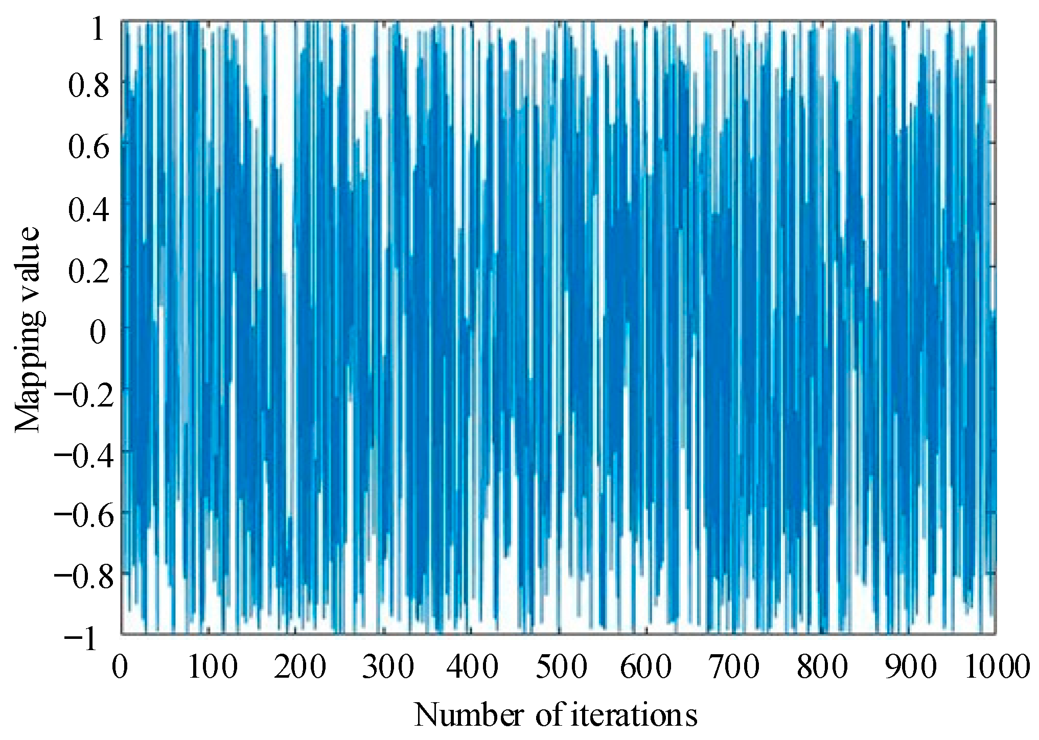
where k is the number of iterations. The distribution of 1000 iterations of Chebyshev mapping is shown in Figure 5.

From Figure 5, it can be seen that the Chebyshev mapping is uniformly distributed between −1 and 1. The initial population generation method of BPSO based on Chebyshev mapping is as follows:

$$x_{i,d}^0=\{\begin{array}{ll}2\mathrm{rand}-1& i=1\\ \cos (i\times \arccos x_{i-1,d})& i>1\end{array}$$

(20)

$$x_{i,d}^1=\{\begin{array}{l}1x_{i,d}^0\ge 0.5\\ 0x_{i,d}^0<0.5\end{array}$$

(21)

where x_i,d denotes the value of the dth position of the ith particle, and rand is a random number with values ranging from 0 to 1. Equation (20) distributes the population particles uniformly in [−1, 1] based on the Chebyshev mapping. Equation (21) discretizes the particle displacement to generate the initial population of BPSO.

3.2.3. Mutation Strategy

The mutation operation can maintain the diversity of the population and prevent the occurrence of premature convergence. In this paper, the mutation strategy of GA is incorporated into the iterative process of BPSO to improve the global search capability of the algorithm [34]. The mutation particle pool N_pool is generated with mutation probability pm at the end of particle update, and the particles from N_pool are sequentially taken out to perform mutation operation, as shown in Equations (22) and (23).

$$i=\{\begin{array}{l}1r_3<p_m\\ 0r_3\ge p_m\end{array}$$

(22)

$$x_{i,d}^k=\{\begin{array}{l}\overline{x_{i,d}^k}i=1\&r_4<{\rho }_m\\ x_{i,d}^{k}else\end{array}$$

(23)

where $x_{i,d}^k$ is the value of the dth position of particle i at the kth iteration, ${\rho }_m$ is the probability of variation of the dth position of the particle, $\overline{x_{i,d}^k}$ is the logical “NOT” operation on $x_{i,d}^k$, and r₃ and r₄ are random numbers with values ranging from 0 to 1.

4. Fault Section Location Method

In addition to the increasing load, the distribution network in actual engineering mainly adopts a network structure of multiple sections to limit the faults to a smaller area and improve the reliability of the power supply. However, the increase in the number of sections increases the number of feeder sections in the distribution network area, thus expanding the solution space for fault section location. This seriously affects the computational efficiency and accuracy of the algorithm. For this reason, this section investigates a dimensionality reduction strategy for fault section location. Firstly, we define a fault confidence factor to characterize the degree of fitting of the section fault hypothesis to the fault information and use it as a basis for proposing a screening rule for the fault candidate scenarios. The fault candidate scenarios are composed into a solution space to reduce the fault search dimension.

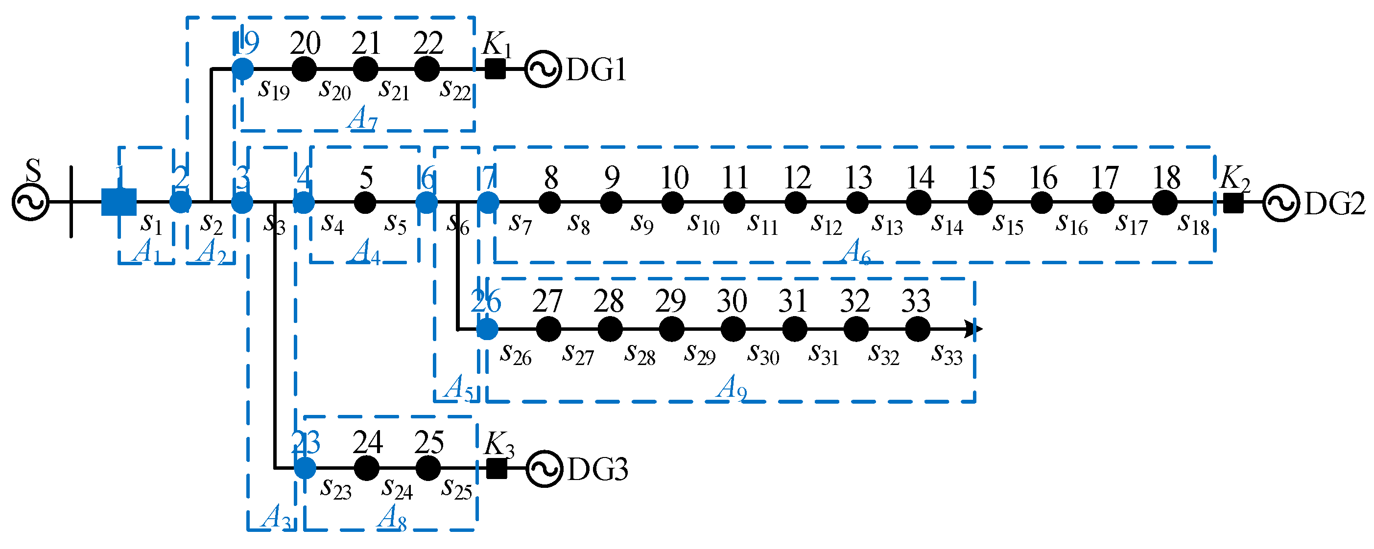
For the sake of convenience, the concepts “upstream” and “downstream” are applied to represent the location relationship between sections within an area in this paper. The IEEE 33-node distribution network shown in Figure 6 is used as an example to illustrate the location relationship between sections. According to the area division method described in Section 2.2.2 of this paper, the area division results of this distribution network are marked in the figure. The port nodes and area are marked in blue. In area A₉, compared with section s₃₁, section s₂₈ is closer to the main power source; therefore, s₂₈ is located upstream of s₃₁ and s₃₁ is located downstream of s₂₈.

In addition, the notation of this section is unified as follows: the boundary node near the main power supply side of the area is designated as u, the boundary node at the other end is designated as d, and the symbol A_u,d is used to represent the area. In particular, since the area containing the end of the power supply does not have the boundary node d, the feeder section located at the end of the power supply can be used instead of the boundary node d to represent the area. For example, for area A₈, let d = s₂₅, $A_8=A_{23,s_{25}}$. ${\mathit{X}}_{u,d}^{*}$ is used to represent the fault candidate scenario of $A_{u,d}^{+}$. ${\mathit{S}}_{\alpha ,\beta }$ and ${\mathit{N}}_{\alpha ,\beta }$ are used to represent the set of sections and nodes between α and β, respectively, where α and β can denote either sections or nodes. Taking area A₈ as an example, the notation correspondence is shown in

Table 3. Correspondence of the notation of area A₈.

u	d	A8	Su,d	${\mathit{S}}_{{\mathit{s}}_{23},{\mathit{s}}_{25}}$	Nu,d	${\mathit{N}}_{\mathit{u},{\mathit{s}}_{24}}$	${\mathit{N}}_{{\mathit{s}}_{23},\mathit{d}}$	${\mathit{N}}_{{\mathit{s}}_{23},{\mathit{s}}_{25}}$
23	s25	$A_{23,s_{25}}$	{s23, s24, s25}	{s23, s24, s25}	{23, 24, 25}	{23, 24}	{24, 25}	{24, 25}

.

According to whether the fault area has an upstream or downstream power supply, the fault area can be divided into two types of power supply: a single power supply and a dual power supply. According to the direction of the short-circuit current, a single power supply fault area can be further divided into a positive-supply fault area and negative-supply fault area.

Take the distribution network shown in Figure 6 as an example to illustrate the rules for determining the type of fault area. Suppose area A₉ is determined as a fault area. If A₉ can receive the positive short-circuit current provided by the main power supply S, then A₉ is the positive power supply fault area, recorded as $A_9^{+}$. Suppose area A₃ and area A₈ are both determined to be fault areas: in this case, the short-circuit power provided by the main power supply S is cut off by the fault area A₃. Then, A₈ can receive the negative short-circuit current provided by distributed generation DG3, making A₈ the negative power supply fault area, which is recorded as $A_8^{-}$. Supposing only area A₈ is determined as the fault area: A₈ can receive the bi-directional short-circuit current provided by S and DG3, making A₈ the dual power supply fault area, which is noted as $A_8^D$. In this section, the screening rules for the fault candidate scenarios are discussed according to the type of fault area.

It should be noted that some areas in the distribution network may contain only one section (e.g., areas A₁, A₂, A₃, and A₅ of the distribution network, shown in Figure 6). When this type of area is determined to be a fault area, the section inside it can be directly located as a fault section without further screening of fault candidate scenarios.

4.1. Fault Screening Rules for Positive Power Supply Fault Area

For a positive power supply fault area, $A_{u,d}^{+}$, set section $s_k\in {\mathit{S}}_{u,d}$. The positive fault confidence factor for s_k is represented by the variable $Z_k^{+}$, which is defined as shown in Equation (24).

$$Z_k^{+}={\displaystyle \sum _{j\in N_{u,s_k}}(I_j^1-I_j^0)}$$

(24)

where $I_j^1$ indicates whether node j reported positive fault current information when $I_j^{}=1$, $I_j^1=1$; otherwise, $I_j^1=0$. $I_j^0=0$ indicates whether node j did not report fault information when $I_j^{}=0$, $I_j^0=1$; otherwise, $I_j^0=0$.

Rule 1 provides the fault screening rules for a positive power supply fault area.

Rule 1: If the section with the largest positive fault confidence factor in the positive power supply fault area $A_{u,d}^{+}$ is section s_p, then the fault candidate scenario ${\mathit{X}}_{u,d}^{*}$ of $A_{u,d}^{+}$ is determined by Equation (25).

$${\mathit{X}}_{u,d}^{*}(k)=\{\begin{array}{l}1s_k=s_p\\ 0\mathrm{others}\end{array}$$

(25)

From Equation (25), it can be seen that there is only one fault candidate scenario for the positive power supply fault area $A_{u,d}^{+}$. Therefore, ${\mathit{X}}_{u,d}^{*}$ can be directly output as the result of the fault section location, i.e., it is decided that section s_p is the fault section.

Take the distribution network shown in Figure 6 as an example to illustrate the fault screening rules for positive power supply fault area. Suppose a fault occurs in section s₂₈ and the fault information reported by FTU is [I₁~I₃₃] = [1 1 1 1 1 1 −1 −1 −1 −1 −1 −1 −1 −1 −1 −1 −1 −1 −1 −1 −1 −1 −1 −1 −1 1 1 1 0 0 0 0 0]; according to the fault area location method described in Section 3, A₉ is determined to be the fault area, and the fault section location operation commences. A₉ is the positive power supply fault area, the fault information of its internal nodes 26~33 is extracted [I₂₆~I₃₃] = [1(I₂₆) 1(I₂₇) 1(I₂₈) 0(I₂₉) 0(I₃₀) 0(I₃₁) 0(I₃₂) 0(I₃₃)], and the positive fault confidence factor is calculated according to Equation (24). Taking section s₃₀ as an example, the calculation process and result are shown in Equation (26).

$$\begin{array}{lll}{Z}_{30}^{+}& =& {\displaystyle \sum _{j\in N_{26,s_{30}}}(I_j^1-I_j^0)}=\left(I_{26}^1-I_{26}^0\right)+\left(I_{27}^1-I_{27}^0\right)+\left(I_{28}^1-I_{28}^0\right)+\left(I_{29}^1-I_{29}^0\right)+\left(I_{30}^1-I_{30}^0\right)\\ & =& \left(1-0\right)+\left(1-0\right)+\left(1-0\right)+\left(0-1\right)+\left(0-1\right)=1\end{array}$$

(26)

Similarly, the positive fault confidence factors of other sections in A9 can be calculated as: $Z_{26}^{+}=1$, $Z_{27}^{+}=2$, $Z_{28}^{+}=3$, $Z_{29}^{+}=2$, $Z_{31}^{+}=0$, $Z_{32}^{+}=-1$, and $Z_{33}^{+}=-2$. From the calculation result, we can see that section s₂₈ has the largest positive fault confidence factor. Therefore, the fault candidate scenario is ${\mathit{X}}_{26,s_{33}}^{*}=\left[x_{26}\text{~}{x}_{33}\right]=\left[00100000\right]$. Since there is only one fault candidate scenario, section s₂₈ is directly determined as a fault section.

4.2. Fault Screening Rules for Negative Power Supply Fault Area

For a negative power supply fault area $A_{u,d}^{-}$, set section $s_k\in {\mathit{S}}_{u,d}$. The negative fault confidence factor for s_k is represented by the variable $Z_k^{-}$, which is defined as shown in Equation (27).

$$Z_k^{-}={\displaystyle \sum _{j\in N_{s_k,d}}(I_j^{-1}-I_j^0)}$$

(27)

where $I_j^{-1}$ indicates whether node j reported negative fault current information when $I_j^{}=-1$, $I_j^{-1}=1$; otherwise, $I_j^{-1}=0$.

In particular, for a feeder section s_e located at the end of the power supply, the negative fault confidence factor $Z_e^{-}=0$ for s_e can be made to work at this time due to ${\mathit{N}}_{s_e,s_e}=Ø$, and the subsequent analysis of the case shows that this treatment is correct.

Rule 2 provides the fault screening rules for the negative power supply fault area.

Rule 2: If the section with the largest negative fault confidence factor in the negative power supply fault area, $A_{u,d}^{-}$, is section s_q, then the fault candidate scenario ${\mathit{X}}_{u,d}^{*}$ of $A_{u,d}^{-}$ is determined by Equation (28).

$${\mathit{X}}_{u,d}^{*}(k)=\{\begin{array}{l}1s_k=s_q\\ 0\mathrm{others}\end{array}$$

(28)

From Equation (28), it can be seen that there is only one fault candidate scenario for the negative power supply fault area. Therefore, ${\mathit{X}}_{u,d}^{*}$ can be directly output as the result of the fault section location, i.e., it is decided that the section s_q is the fault section.

4.3. Fault Screening Rules for Dual Power Supply Fault Area

Compared with the single power supply fault area, the fault characteristics of the dual power supply fault area are more complex, and the fault candidate scenarios need to be determined through two processes: a preliminary screening and a secondary screening.

4.3.1. Preliminary Screening

The task of the preliminary screening is to determine the range of sections within the fault area where faults are likely to occur. This can be achieved through the calculation and comparison of fault confidence factors.

For the dual power supply fault area, $A_{u,d}^D$, set section $s_k\in {\mathit{S}}_{u,d}$. To distinguish it from the single power supply fault area, apply the variables $Z_k^{D+}$ and $Z_k^{D-}$ to represent the positive fault confidence factor and negative fault confidence factor of the sections, respectively. $Z_k^{D+}$ and $Z_k^{D-}$ are defined as shown in Equations (29) and (30).

$$Z_k^{D+}={\displaystyle \sum _{j\in N_{u,s_k}}(I_j^1-I_j^0-I_j^{-1})}$$

(29)

$$Z_k^{D-}={\displaystyle \sum _{j\in N_{s_k,d}}(I_j^{-1}-I_j^1-I_j^0)}$$

(30)

As in the case of the negative power supply fault area, for feeder section s_e located at the end of the power supply, the negative fault confidence factor $Z_e^{D-}=0$ of s_e can be made to work at this time due to ${\mathit{N}}_{s_e,s_e}=Ø$. The subsequent analysis of the case shows that this treatment is correct.

Rule 3 provides the method of determining the range of section faults within the dual power supply fault area.

Rule 3. If the section with the largest positive fault confidence factor and negative fault confidence factor in the dual power supply fault area, $A_{u,d}^D$, are s_p and s_q, respectively, then the fault sections in the fault candidate scenario ${\mathit{X}}_{u,d}^{*}$ should be between s_p and s_q (including s_p and s_q), i.e., the fault section in ${\mathit{X}}_{u,d}^{*}$ should belong to the set ${\mathit{S}}_{s_p,s_q}$.

In particular, when s_p = s_q, a single fault section can be identified in area $A_{u,d}^D$ due to ${\mathit{S}}_{s_p,s_q}=s_p=s_q$, according to Rule 3. The fault candidate scenario ${\mathit{X}}_{u,d}^{*}$ is then determined by Equation (31).

$${\mathit{X}}_{u,d}^{*}(k)=\{\begin{array}{l}1s_k=s_p=s_q\\ 0\mathrm{others}\end{array}$$

(31)

From Equation (31), we can see that when s_p = s_q, there is only one fault candidate scenario. Therefore, ${\mathit{X}}_{u,d}^{*}$ can be directly output as the result of the fault section location, i.e., we decide that section s_p (s_q) is the fault section. If s_p ≠ s_q, we need to perform a secondary screening of the sections in the set ${\mathit{S}}_{s_p,s_q}$.

4.3.2. Secondary Screening

The task of secondary screening is to determine the fault candidate scenarios based on the preliminary screening, which needs to be achieved by the calculation and comparison of the fault comparability degree.

Let s_p and s_q be the sections with the largest positive fault confidence factor and negative fault confidence factor in the dual power supply fault area $A_{u,d}^D$, respectively, and s_p ≠ s_q. Let the positive fault comparability degree and negative fault comparability degree of sections be represented by the variables $Y_k^{+}$ and $Y_k^{-}$, respectively. $Y_k^{+}$ and $Y_k^{-}$ are defined as shown in Equations (32) and (33).

$$Y_k^{+}={\displaystyle \sum _{j\in N_{s_p,s_k}}(I_j^1-I_j^0)}$$

(32)

$$Y_k^{-}={\displaystyle \sum _{j\in N_{s_k,s_q}}(I_j^{-1}-I_j^0)}$$

(33)

Rule 4 provides the screening rules for the fault candidate scenarios when s_p ≠ s_q, as follows:

• Step 1: Calculate the positive fault comparability degree and negative fault comparability degree of the section in the set ${\mathit{S}}_{s_p,s_q}$ according to Equations (32) and (33);
• Step 2: The set of sections with non-negative values for the positive fault comparability degree is S⁺, and the set of section s with non-negative values for the negative fault comparability degree is S⁻;
• Step 3: Determine if S⁺∩S⁻ is the empty set; if not, go to step 4; otherwise, go to step 5;
• Step 4: Take the sections from the set S⁺∩S⁻ as the fault sections of ${\mathit{X}}_{u,d}^{*}$, and construct the fault candidate scenarios in turn. Suppose the number of elements in S⁺∩S⁻ is m₁. There are then m₁ fault candidate scenarios that can be identified in this step;
• Step 5: Take out the section s_k from the set S⁺ and find the section s_kd located downstream of s_k from the set S⁻. Use s_k and s_kd as the fault sections of ${\mathit{X}}_{u,d}^{*}$ to construct the fault candidate scenarios. Assuming that for the section s_k in S⁺, there are m_k sections downstream of s_k in S⁺. There are then ${\displaystyle \sum _{s_k\in S^{+}}{m}_k}$ fault candidate scenarios that can be identified in this step;
• Step 6: Output the screening results of the fault candidate scenarios.

In fact, when s_p ≠ s_q (excluding the extreme case in which the fault information for multiple nodes in the fault area are distorted at the same time), in general, only the fault comparability degree of section s_p and section s_q in the set ${\mathit{S}}_{s_p,s_q}$ satisfy $Y_p^{+}\ge 0$ and $Y_q^{-}\ge 0$, respectively. It can be seen that the fault candidate scenarios screened by Rule 4 are very few (usually only 1), so the objective function $f({\mathit{X}}_{u,d}^{*})$ of the fault candidate scenarios ${\mathit{X}}_{u,d}^{*}$ can be calculated according to Equation (5), and the smallest $f({\mathit{X}}_{u,d}^{*})$ of ${\mathit{X}}_{u,d}^{*}$ is used as the result of fault section location.

The distribution network shown in Figure 6 is used as an example to illustrate the fault screening rules of the dual power fault area and its dimensionality reduction effect.

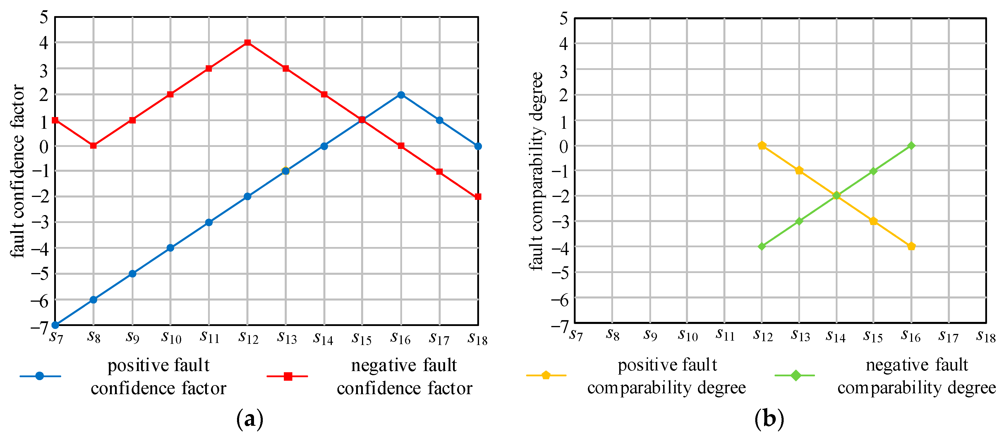
Suppose section s₁₂ and section s₁₆ fail at the same time. In actual engineering, FTUs are mostly installed outdoors and work in harsh environments, and the reported fault information may be misreported or missed, and other distortions may occur. Therefore, in the case of a small-scale distortion of information, it should be able to output the correct location results as much as possible. To assess the fault-tolerance ability of the fault section location method in this example, we assume that node 8 misses the fault information, i.e., I₈ = 1→0. At this time, the fault information reported by FTU is [I₁~I₃₃] = [1 1 1 1 1 1 1 0 1 1 1 1 1 0 0 0 0 0 0 −1 −1 −1 −1 −1 −1 −1 −1 −1 −1 −1 0 0 0 0 0 0 0 0 0 0]. According to the fault area location method described in Section 3, A₆ is determined to be a fault area, and the fault section location operation is initiated. A₆ is a dual power supply fault area, and the preliminary screening is performed first. The fault information of nodes 7~18 inside A₆ [I₇~I₁₈] = [1(I₇) 0(I₈) 1(I₉) 1(I₁₀) 1(I₁₁) 1(I₁₂) 0(I₁₃) 0(I₁₄) 0(I₁₅) 0(I₁₆) −1(I₁₇) −1(I₁₈)] are extracted, and the fault confidence factor is calculated according to Equations (29) and (30). Taking section s₁₂ as an example, the calculation process and results of $Z_{12}^{D+}$ and $Z_{12}^{D-}$ are shown in Equations (34) and (35).

$$\begin{array}{lll}{Z}_{12}^{D+}& =& {\displaystyle \sum _{j\in N_{7,s_{12}}}(I_j^1-I_j^0-I_j^{-1})}=\left(I_7^1-I_7^0-I_7^{-1}\right)+\left(I_8^1-I_8^0-I_8^{-1}\right)+\left(I_9^1-I_9^0-I_9^{-1}\right)\\ & +& \left(I_{10}^1-I_{10}^0-I_{10}^{-1}\right)+\left(I_{11}^1-I_{11}^0-I_{11}^{-1}\right)+\left(I_{12}^1-I_{12}^0-I_{12}^{-1}\right)\\ & =& \left(1-0-0\right)+\left(0-1-0\right)+\left(1-0-0\right)+\left(1-0-0\right)+\left(1-0-0\right)+\left(1-0-0\right)=4\end{array}$$

(34)

$$\begin{array}{lll}{Z}_{12}^{D-}& =& {\displaystyle \sum _{j\in N_{s_{12},s_{18}}}\left(I_j^{-1}-I_j^1-I_j^0\right)}=\left(I_{13}^{-1}-I_{13}^1-I_{13}^0\right)+\left(I_{14}^{-1}-I_{14}^1-I_{14}^0\right)+\left(I_{15}^{-1}-I_{15}^1-I_{15}^0\right)\\ & +& \left(I_{16}^{-1}-I_{16}^1-I_{16}^0\right)+\left(I_{17}^{-1}-I_{17}^1-I_{17}^0\right)+\left(I_{18}^{-1}-I_{18}^1-I_{18}^0\right)\\ & =& \left(0-0-1\right)+\left(0-0-1\right)+\left(0-0-1\right)+\left(0-0-1\right)+\left(1-0-0\right)+\left(1-0-0\right)=-2\end{array}$$

(35)

Similarly, the results of the fault confidence factors of other sections in A₆ are as shown in Figure 7a.

From Figure 7a, it can be seen that section s₁₂ has the largest forward fault confidence factor, and section s₁₆ has the largest negative fault confidence factor. Therefore, the fault section in the fault candidate scenarios ${\mathit{X}}_{7,s_{18}}^{*}$ should be between s₁₂ and s₁₆. Since s₁₂ ≠ s₁₆, a secondary screening is required. The fault comparability degree of the section in ${\mathit{S}}_{s_{12},s_{16}}$ is calculated according to Equations (32) and (33). Taking section s₁₄ as an example, the calculation process and results of $Y_{14}^{+}$ and $Y_{14}^{-}$ are shown in Equations (36) and (37).

$$Y_{14}^{+}={\displaystyle \sum _{j\in N_{s_{12},s_{14}}}\left(I_j^1-I_j^0\right)}=\left(I_{13}^1-I_{13}^0\right)+\left(I_{14}^1-I_{14}^0\right)=\left(0-1\right)+\left(0-1\right)=-2$$

(36)

$$Y_{14}^{-}={\displaystyle \sum _{j\in N_{s_{14},s_{16}}}\left(I_j^{-1}-I_j^0\right)}=\left(I_{15}^{-1}-I_{15}^0\right)+\left(I_{16}^{-1}-I_{16}^0\right)=\left(0-1\right)+\left(0-1\right)=-2$$

(37)

Similarly, the results of the fault comparability degree of other sections in A₆ are shown in Figure 7b.

From Figure 7b, we can see that the positive fault comparability degree of section s₁₂ is non-negative and the set S⁺ = {s₁₂}. The negative fault comparability degree of section s₁₆ is non-negative and the set S⁻ = {s₁₆}. According to Rule 4, section s₁₂ has been taken out and section s₁₆ is found to be located downstream of s₁₂; s₁₂ and s₁₆ are selected as the fault sections to construct the fault candidate scenario as ${\mathit{X}}_{7,s_{18}}^{*}=\left[x_7~x_{18}\right]=\left[000001000100\right]$. Since there is only one fault candidate scenario, we can directly output ${\mathit{X}}_{7,s_{18}}^{*}$ as the result of fault section location and determine section s₁₂ and section s₁₆ as the fault sections.

The following is an analysis of the dimensionality reduction effect. Without fault screening, the solution space is composed of the operation states of sections s₇~s₁₈ in fault area A₆. Since each section contains both fault and normal operation states, the size of the solution space is 2¹², and there is only one fault candidate scenario after filtering. It can be seen that the introduction of fault filtering reduces the search dimension of the fault sections by (2¹² −1)/2¹² = 99.98%.

Large-scale distribution networks usually contain a large number of feeder sections within the area, and the size of the solution space for fault section location links is substantial if they are not filtered by faults. The exhaustive enumeration of all possible fault scenario seriously reduces the computational efficiency. While locating fault sections with the help of intelligent algorithms can guarantee computational efficiency to a certain extent, local convergence may occur, and accuracy cannot be guaranteed. This section achieves a reduction in dimensionality with the help of fault filtering and avoids the random intelligent search operation. It is foreseeable that the fault filtering method proposed in this section has great potential for improving the computational efficiency and accuracy of fault location in the context of large-scale active distribution networks.

5. Fault Location Process

The implementation flow of the fault location method proposed in this paper is shown in Figure 8. The specific steps are as follows:

• Step 1: Read the distribution network information and set the algorithm parameters. Build the hierarchical optimization model. Collect the information reported by the FTU;
• Step 2: Extract the fault information of the port nodes and start the fault area location link. Initialize the velocity and displacement of the particle population based on Equations (20) and (21). Set the iteration number of the algorithm t = 1, and set the maximum number of iterations allowed by the algorithm to t_max;
• Step 3: Calculate the objective function of the particle according to Equation (5). Determine the individual extremum P_i and the population extremum G. Denote the value of the objective function corresponding to the population extremum G as f(G). Let t = t + 1;
• Step 4: Update the particle population according to Equations (15)–(17) and perform mutation operations on the population according to Equations (22) and (23);
• Step 5: Judge whether the convergence condition is reached according to Equation (18) (i.e., whether the maximum number of iterations has been reached (t > t_max) or the objective function of the population extreme value point reaches the optimal value (f(G) = 0.5)). If it is satisfied, output the population extreme value point G as the result of fault area location. Otherwise, go to Step 3;
• Step 6: Determine the type of the fault area. If it has only upstream power, go to Step 7; if it has only downstream power, go to Step 8; otherwise, go to Step 9;
• Step 7: Calculate the positive fault confidence factor according to Equation (24), and determine the section with the largest value as the fault section;
• Step 8: Calculate the negative fault confidence factor according to Equation (27), and determine the section with the largest value as the fault section;
• Step 9: Calculate the fault confidence factor according to Equations (29) and (30), and obtain the section s_p and s_q with the largest positive and negative fault confidence factors. If s_p = s_q, then section s_p(s_q) will be judged as the fault section; otherwise, go to Step 10;
• Step 10: Calculate the fault comparability degree of the section according to Equations (32) and (33), and screen the fault candidate scenarios according to Rule 4;
• Step 11: The fault candidate scenario with the smallest objective function is used as the location result, and the fault section is determined.

6. Simulation Analysis

In order to verify the effectiveness of the algorithms in this paper, this section simulates and tests the fault location of the algorithms in this paper using an IEEE 33-node distribution network and an IEEE 69-node distribution network as examples. They are compared with other algorithms in terms of accuracy, fault tolerance, and computational efficiency, respectively. The algorithms involved in the comparison include the binary particle swarm optimization algorithm (Algorithm 1) [19], improved binary particle swarm optimization algorithm (Algorithm 2), the immune optimization algorithm (Algorithm 3) [24], and the bald eagle search algorithm (Algorithm 4) [25]. The specific fault location methods of various algorithms are shown in

Table 4. Fault location methods for various algorithms.

Algorithm Number	Fault Location Method
Algorithm 1	A single-level fault location model is used to locate the fault section by applying the binary particle swarm algorithm (BPSO).
Algorithm 2	A single-layer fault location model is used to locate the fault section by applying the improved binary particle swarm optimization algorithm (IBPSO) in this paper.
Algorithm 3	Using the traditional hierarchical model, the immune optimization algorithm is applied to locate the fault area and fault section.
Algorithm 4	Using the traditional hierarchical model, the bald eagle search algorithm is applied to locate the fault area, and the fault section is then determined by applying the exhaustive method.
Algorithm 5	The algorithm presented in this paper, using the improved hierarchical optimization model, applies the IBPSO to locate the fault area and locate the fault section by screening the fault candidate scenarios based on the fault confidence factor.

. The simulated experimental environment in this paper was based on an Intel(R) Core (TM) i7-1260U processor with a 2.10 GHz CPU, 16.00 G of RAM, and a Windows 11 (64-bit) operating system.

6.1. IEEE 33-Node Distribution Network

The IEEE 33-node distribution network is shown in Figure 6. It has one main power source, three distributed power sources, one substation distribution side outgoing circuit breaker, three DG grid-connected switches, 32 sectional switches and 33 feeder sections, and the DG is connected to the distribution network through the end of the supply. The DGs are motor-type DGs, and the short-circuit capacity is set to 20% of the main short-circuit capacity. K₁~K₃ denote DG-grid-connected switches. Suppose that the communication network is intact, and all FTUs report sound fault information in addition to the set information distortion point. The parameters involving the intelligent optimization algorithm are set as follows: the population size of the algorithm is set to 50, and the maximum number of iterations is 30.

6.1.1. Accuracy

To test the accuracy of the algorithm, multiple fault types such as single fault, multiple faults, and end-of-supply faults are set. The algorithm is run 100 times in a loop, and the ratio of the number of correct locations to the total number of runs is taken to describe the accuracy of the algorithm in which K = [K₁, K₂, K₃] indicates the dynamic throwing and cutting of distributed power DG1~DG3. K_i = 1 when the DGi is put into operation; otherwise, K_i = 0. The test results of the accuracy of each algorithm are shown in

Table 5. Accuracy test results.

Equipment Number	K	Preset Fault Section	Accuracy (%)
			Algorithm 1	Algorithm 2	Algorithm 3	Algorithm 4	Algorithm 5
1	[0, 1, 1]	s3	88	90	100	100	100
2	[0, 0, 0]	s22	87	91	100	100	100
3	[1, 1, 1]	s10	76	86	99	100	100
4	[1, 0, 1]	s26	70	75	100	100	100
5	[1, 1, 1]	s4, s32	72	88	Misjudgment	Misjudgment	100
6	[1, 1, 0]	s14, s29	92	90	98	100	100
7	[0, 0, 0]	s18, s24	82	82	99	100	100
8	[1, 0, 0]	s5, s16	83	85	Misjudgment	Misjudgment	100

.

As can be seen from Table 5, the correct rate of Algorithm 1 is approximately 80%. Thanks to the BPSO improvement strategy proposed in this paper, the accuracy of Algorithm 2 is approximately 5% higher than that of Algorithm 1. On the other hand, the dimensionality reduction effect of the hierarchical model has a more obvious effect on the accuracy improvement, where the accuracies of Algorithm 3 and Algorithm 4 are close to 100% for most of the fault cases. However, due to the influence of the power coupling phenomenon of the T-section, Algorithm 3 and Algorithm 4 misjudge the fault cases of serial numbers 5 and 8. The hierarchical model constructed in this paper achieves decoupled identification of faults on T-sections and branches. Therefore, it can accurately identify complex fault cases in which both the upstream and downstream branches of the T-sections fail at the same time while also achieving a dimensionality reduction. The test results confirm that Algorithm 5 achieves a 100% accuracy for the fault cases in Table 5.

The fault case 5 in Table 5 is used as an example to illustrate the execution process of the algorithm in this paper. In fault case 5, both upstream and downstream branches of T-type section s₆ fail at the same time. The algorithm first starts the fault area location operation. The fault information of the port nodes [1(I₁) 1(I₂) 1(I₃) 1(I₄) −1(I₆) −1(I₇) −1(I₁₉) −1(I₂₃) 1(I₂₆)] is extracted. Running the IBPSO algorithm determines the fault areas to be A₇ and A₉. Next, the fault section location operation is initiated. The fault section A₇ is determined to be a dual power supply fault area, and the fault information of nodes 4~6 inside A₇ are extracted [1(I₄) −1(I₅) −1(I₆)]. The fault confidence factors are calculated for the sections s₄, s₅, and the results are as follows: $Z_4^{D+}=1$, $Z_5^{D+}=0$, $Z_4^{D-}=2$, $Z_5^{D-}=1$. The section with the largest positive and negative fault confidence factor is s₄; therefore, s₄ is determined to be the fault section. The fault section A₉ is determined to be a positive power supply fault area, and the fault information of nodes 26~33 inside A₉ is extracted [1(I₂₆) 1(I₂₇) 1(I₂₈) 1(I₂₉) 1(I₃₀) 1(I₃₁) 1(I₃₂) 0(I₃₃)]. The positive fault confidence factors for the sections s₂₆~s₃₃ are calculated, and the results are as follows: $Z_{26}^{+}=1$, $Z_{27}^{+}=2$, $Z_{28}^{+}=3$, $Z_{29}^{+}=4$, $Z_{30}^{+}=5$, $Z_{31}^{+}=6$$Z_{31}^{+}=6$, $Z_{32}^{+}=7$, $Z_{33}^{+}=6$. The section with the largest positive fault confidence factor is s₃₂; therefore, s₃₂ is determined to be the fault section. The fault location operation is completed and the fault sections s₄ and s₃₂ are output.

6.1.2. Fault Tolerance

In actual engineering, the FTU and communication equipment are mostly installed outdoors, which makes the equipment susceptible to lightning, external forces, and electromagnetic influences, and the reported fault information may be misreported or missed, and other distortions may occur. Therefore, to ensure the reliability of fault identification, the fault tolerance of the algorithm should be improved as much as possible in the case of small-scale aberrations in the reported information of FTU.

In this section, the distortion signals of nodes 1 to 3 are set to simulate the distortion of the actual project to check the fault tolerance of the algorithm. The simulation results are shown in

Table 6. Fault Tolerance results.

Equipment Number	Preset Fault Section	Preset Information Distortion	Accuracy (%)
			Algorithm 1	Algorithm 2	Algorithm 3	Algorithm 4	Algorithm 5
1	s32	I27: 1 → 0	82	83	100	100	100
2	s6	I29: 0 → 1, I9: −1 → 0	84	85	100	100	100
3	s12	I16: −1 → 0	78	78	99	100	100
4	s19	I7: −1 → 1	73	80	100	100	100
5	s20, s24	I28: 0 → 1	70	76	100	100	100
6	s5, s10	I13: −1 → 0, I30: 0 → 1	73	72	98	100	100
7	s12, s16	I5: 1 → 0	79	81	99	100	100
8	s15, s26	I2: 1 → 0, I11: 1 → −1, I25: −1 → 0	73	79	99	100	100

. Suppose that all DGs are put into operation.

The fault information distortion causes the values of the objective function in the solution space to become closer, thus increasing the probability of local convergence of the intelligent algorithm. As can be seen from Table 6, the accuracies of Algorithm 1 and Algorithm 2, which are based on the single-layer model, are reduced to approximately 75% and 79%, respectively. Algorithm 3, Algorithm 4, and Algorithm 5, which are based on the hierarchical model, still maintain high accuracy rates, and algorithm 5 maintains a 100% accuracy rate for the fault conditions in Table 6. This shows that the algorithm in this paper has a high fault-tolerance ability.

6.2. IEEE 69-Node Distribution Network

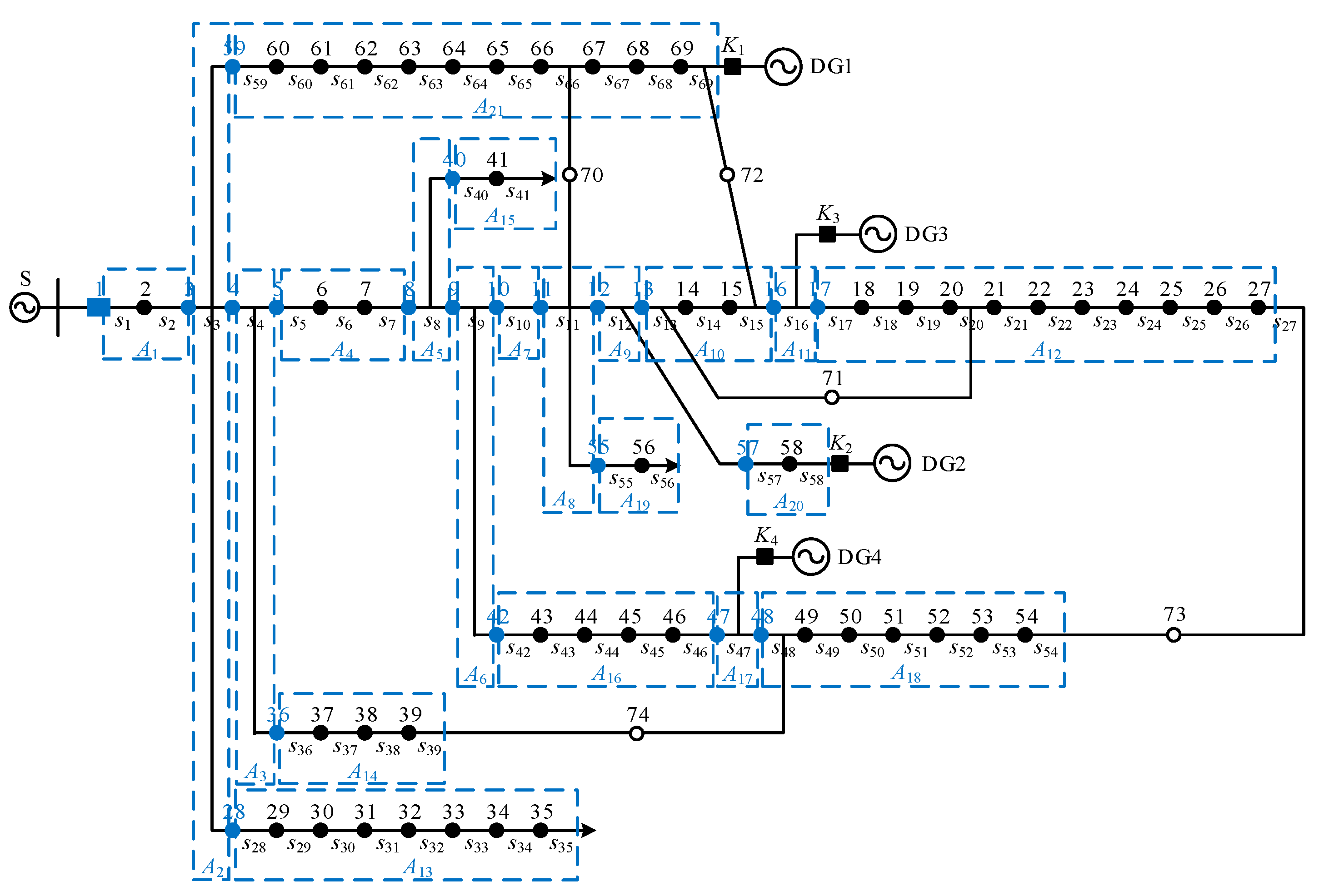
The IEEE 69-node distribution network is shown in Figure 9. It has one main power source, four distributed power sources, one substation distribution side outlet circuit breaker, four DG-grid-connected switches, sixty-eight sectional switches, five interconnection switches and sixty-nine feeder sections, and the DG is connected to the distribution network through the end of the supply and the “T” connection form. The DGs are motor-type DGs, and the short-circuit capacity is set to 20% of the main short-circuit capacity. K₁~K₄ denote DG-grid-connected switches. Suppose that the communication network is intact, and all the FTUs report sound fault information in addition to the set information distortion point. The results of the area division of the distribution network are shown in Figure 9. In Figure 9, the port nodes and the area are marked in blue. The parameters of the intelligent optimization algorithm are set as follows: the population size of the algorithm is set to 100, and the maximum number of iterations is 70.

To further verify the adaptability of the algorithm in this paper in large-scale distribution networks, this section provides a comprehensive comparison of the accuracy and computational efficiency of the algorithm under various fault scenarios. The test cases in this section are shown in

Table 7. Test cases for IEEE 69-node distribution network.

Equipment Number	[K1, K2, K3, K4]	Preset Fault Section	Preset Information Distortion
1	[1, 1, 1, 1]	s27	-
2	[0, 1, 1, 1]	s33	I15: -1 → 0
3	[0, 0, 0, 0]	s44	I6: 1 → 0, I23: 0 → −1, I64: 0 → 1
4	[1, 0, 0, 1]	s54	I7: 1 → −1, I14: 0 → 1, I26: 0 → −1, I44: 1 → −1, I50: −1 → 1
5	[0, 0, 1, 1]	s7, s40	-
6	[1, 0, 1, 0]	s64, s69	I44: −1 → 1, I61: 1 → 0
7	[1, 1, 1, 0]	s5, s58	I1: 1 → 0, I19: 0 → −1, I20: 0 → 1, I32: 0 → 1
8	[1, 1, 0, 1]	s43, s52	I4: 1 → − 1, I46: − 1 → 0
9	[1, 1, 1, 1]	s35, s66	-
10	[1, 1, 1, 0]	s2, s10, s34	-
11	[1, 1, 1, 1]	s7, s60, s69	I13: −1 → 0, I31: 0 → −1, I63: 0 → 1
12	[0, 0, 0, 0]	s18, s42, s64	I10: 1 → 0, I22: 0 → 1, I25: 0 → −1, I38: 0 → −1

and cover various fault cases such as single fault, multiple faults, sound fault information, and distorted fault information. Among these cases, the dynamic throwing cases of distributed power supplies DG1~DG4 are represented by [K₁, K₂, K₃, K₄]. When DGi is put into operation, K_i = 1; otherwise, K_i = 0.

6.2.1. Accuracy

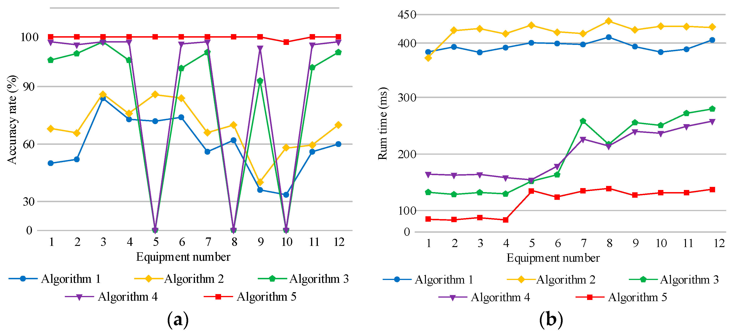
As can be seen from Figure 10a, the accuracies of Algorithm 1 and Algorithm 2 decrease to a large extent, and the accuracy for some test cases has been reduced to less than 50%. This indicates that the single-layer model is not suitable for large-scale distribution networks. Algorithm 3 applies the intelligent algorithm to locate the fault section. With the increase in the number of feeder sections in the distribution network areas, its accuracy decreases to a certain extent. The accuracy of Algorithm 4 is higher than that of Algorithm 3 because Algorithm 4 applies the exhaustive method to locate the fault section and avoids the random search operation. Moreover, Algorithm 3 and Algorithm 4 are affected by the power coupling phenomenon of the T-section, which misjudges the fault cases of serial numbers 5, 8, and 10. In this paper, we avoid the random search operation by screening fault candidate scenarios based on the fault confidence factor. The test results show that, thanks to the above measures, the accuracy of the algorithm in this paper is minimally affected by the network size, and the accuracy reaches 100% in all fault cases in Table 7.

6.2.2. Computational Efficiency

Each algorithm is run 100 times in a loop, and the average time taken for a single run is used as a measure of the computational efficiency of the algorithm. The test results are shown in Figure 10b.

As can be seen from Figure 10b, the computational efficiency of Algorithm 1 is approximately 400 ms, and the computational efficiency of Algorithm 2 is approximately 420 ms. This is due to the fact that the algorithm based on the single-layer model requires iterative operations in a high-dimensional solution space. The hierarchical model has a more obvious effect on the improvement of the computational efficiency. The computational efficiency of Algorithm 3 for single and multiple faults is approximately 132 ms and 260 ms, respectively, and the computational efficiency of Algorithm 4 for single and multiple faults is approximately 162 ms and 239 ms, respectively. In this paper, we further reduce the search dimension of the fault section location by screening fault candidate scenarios. The simulation results show that the computational efficiency of Algorithm 5 for a single fault and for multiple faults is approximately 80 ms and 130 ms, respectively, which is 300 ms higher than the results of Algorithm 1 and Algorithm 2 and approximately 0.5 times higher than the results of Algorithm 3 and Algorithm 4.

7. Conclusions

With the massive switch-on of distributed generation and the rising electricity load, the structure and tide of distribution networks are becoming increasingly large and complex. This leads to great challenges for fault location methods. For this reason, an active distribution network fault location method based on a hierarchical optimization model and fault confidence factor is proposed in this paper. In addition, through the simulation experiments of the IEEE 33-node distribution network and the IEEE 69-node distribution network, the following conclusions can be drawn.

• The hierarchical optimization model constructed in this paper reduces the solution space and provides theoretical support for improving the performance of the algorithm. At the same time, the model achieves the decoupling identification of the T-section and branch faults. It can therefore accurately identify the complex fault condition in which the upstream and downstream branches of the T-section fail at the same time, and it is suitable for solving the problem of a DG connected to the distribution network in “T” mode;
• The optimization of the convergence criterion and the introduction of chaotic maps and mutation strategies reduce the probability of the local convergence of BPSO and effectively improve the accuracy of fault area localization;
• The fault-confidence-factor-based fault candidate scenario screening method further reduces the search dimension of the fault section, effectively improving the accuracy and computational efficiency of fault section location;
• The accuracy and computational efficiency of the algorithm in this paper are minimally affected by the scale of the network. This demonstrates prospects for its application in large-scale, complex active distribution networks.

This paper performs fault location based on the fault current direction uploaded by FTU, which has the advantages of small data communication and high localization efficiency. However, when the number of information distortions exceeds the acceptable number of redundancies for the fault location or when crosstalk occurs for multiple faults, misjudgments or omissions may occur. The development of communication technologies and measurement systems provide a hardware basis for the system to obtain multiple source fault information. Future research can use the short-circuit current amplitude, fault recording, or other transient quantity information to correct the location results of this paper’s method to further improve the reliability of distribution network fault location.

References

1. Li, W.; Li, Y.; Zhang, M.; Deng, Y.; Deng, Y.; Li, J.; Zhu, Q.; Zhang, L.; Zhang, S. A fully decentralized multi-agent fault location and isolation for distribution networks With DGs. IEEE Access 2021, 9, 27748–27757. [Google Scholar] [CrossRef]
2. Lin, Y.; Wang, Z.; Wang, T.; Zheng, B. Discussion on building a stronger first line of defense for grid security. Power Syst. Prot. Control 2022, 50, 170–178. [Google Scholar]
3. Galvez, C.; Abur, A. Fault Location in Active Distribution Networks Containing Distributed Energy Resources (DERs). IEEE Trans. Power Deliv. 2021, 36, 3128–3139. [Google Scholar] [CrossRef]
4. He, Z.; Li, B.; Liao, K.; Hu, S.; Ma, Z.; Li, J.; Ke, Y.; Yang, J. Key technologies for protection and control of novel urban power grids. Proc. CSEE 2020, 40, 6193–6206. [Google Scholar]
5. Li, M.; Zhang, S.; Cheng, H.; Yang, D.; Gao, M.; Ni, Z. Hierarchical fault location method for active distribution network with distributed generations. Proc. CSU-EPSA 2021, 33, 79–87. [Google Scholar]
6. Shen, G.; Zhang, Y.; Qiu, H.; Wang, C.; Wen, F.; Salam, M.; Weng, L.; Zhang, L.; Zhang, S. Fault diagnosis with false and/or missing alarms in distribution systems with distributed generators. Energies 2018, 11, 2579. [Google Scholar] [CrossRef] [Green Version]
7. Wang, S.; Song, L.; Shu, X. Adaptive overcurrent protection of active distribution network with high penetration of distributed generations and multiple loads. High Volt. Eng. 2019, 45, 1783–1794. [Google Scholar]
8. Ji, X.; Zhang, S.; Zhang, Y.; Han, X.; Xiao, Y.; Zeng, R. Fault section location for distribution network based on improved electromagnetism-like mechanism algorithm. Autom. Electr. Power Syst. 2021, 45, 157–165. [Google Scholar]
9. Zhao, Q. Research on Wide Area Protection of Smart Distribution Grid; North China Electric Power University: Beijing, China, 2017. [Google Scholar]
10. Li, G.; Chen, Q.; Zhang, J. Novel faulted section location method for distribution network based on status information of fault indicating equipment. Appl. Sci. 2020, 10, 5910. [Google Scholar] [CrossRef]
11. Xu, B.; Yin, X.; Zhang, Z.; Pang, S.; Li, X. Fault location for distribution network based on matrix algorithm and optimization algorithm. Autom. Electr. Power Syst. 2019, 43, 152–158. [Google Scholar]
12. Guo, L.; Li, F.; Zhao, X.; Zhou, J. Fault zone location in DG-containing distribution networks based on sub-network segmentation. Power Syst. Prot. Control 2020, 48, 76–84. [Google Scholar]
13. Zhao, Q.; Wang, Z.; Dong, W.; Bao, W. Research on fault location in a distribution network based on an immune binary particle swarm algorithm. Power Syst. Prot. Control 2020, 48, 83–89. [Google Scholar]
14. Zheng, T.; Ma, L.; Li, B. Fault section location of active distribution network based on feeder terminal unit information distortion correction. Power Syst. Technol. 2021, 45, 3926–3934. [Google Scholar]
15. Jiao, Y.; Du, S.; Wang, Q.; Chen, C. Information aberrance correction and fault-section location for distribution networks based on the information contradiction theory. Power Syst. Prot. Control 2014, 42, 43–48. [Google Scholar]
16. Guo, Z.; Xu, Q.; Hong, J.; Mao, X. Integer linear programming based fault section diagnosis method with high fault-tolerance and fast performance for distribution network. Proc. CSEE 2017, 37, 786–795. [Google Scholar]
17. Wei, Z.; He, H.; Zheng, Y. A refined genetic algorithm for the fault sections location. Proc. CSEE 2002, 22, 127–130. [Google Scholar]
18. Guo, Z.; Chen, B.; Liu, C.; Xu, K.; Li, J. Fault location of distribution network based on genetic algorithm. Power Syst. Technol. 2007, 31, 88–92. [Google Scholar]
19. Li, C.; He, Z.; Zhang, H.; Gao, H. Fault location for radialized distribution networks based on BPSO algorithm. Power Syst. Prot. Control 2009, 37, 35–39. [Google Scholar]
20. Liu, B.; Wang, F.; Chen, C.; Huang, H.; Dong, X. Harmony search algorithm for solving fault location in distribution networks with DG. Trans. China Electrotech. Soc. 2013, 28, 280–284. [Google Scholar]
21. Guo, Z.; Wu, J. Electromagnetism-like mechanism based fault section diagnosis for distribution network. Proc. CSEE 2010, 30, 34–40. [Google Scholar]
22. Wang, Q.; Jin, T.; Shen, T.; Zhu, S.; Liu, S. A complete analytic model of section location in distribution network based on multi-factor dimensionality deduction. Trans. China Electrotech. Soc. 2019, 34, 3012–3024. [Google Scholar]
23. Wang, Q.; Jin, T.; Tan, H.; Li, Z. The technology on fault location of distribution network based on hierarchical model and intelligent checking algorithm. Trans. China Electrotech. Soc. 2018, 33, 5327–5337. [Google Scholar]
24. Li, W.; Tong, X.; Huang, C.; Peng, Y.; Li, D.; Wang, J. F A fault location method for a distribution network with DG based on a hierarchical location model. Power Syst. Technol. 2022, 50, 160–166. [Google Scholar]
25. Yang, G.; Feng, J.; Liu, X.; Chen, R.; Pan, H.; Yang, Q. Fault location of a distribution network hierarchical model with a distribution generator based on IBES. Power Syst. Prot. Control 2022, 50, 1–9. [Google Scholar]
26. Zhang, R.; Liu, L. Distribution network regionalized fault location based on an improved manta ray foraging optimization algorithm. Electronics 2022, 11, 2342. [Google Scholar] [CrossRef]
27. IEC TR 61850-90-6; Communication Networks and Systems for Power Utility Automation—Part 90-6: Use of IEC 61850 for Distribution Automation Systems. International Electrotechnical Commission: Geneva, Switzerland, 2018; pp. 89–103.
28. Li, Y.; Wang, Z.; Zhao, Q. Distributed fault section location for ADN based on bayesian complete analytic model and multi-factor dimension reduction. Power Syst. Technol. 2021, 45, 3917–3925. [Google Scholar]
29. Li, Z.; Wang, Z.; Zhang, Y.; Qiao, X. Fault section location method for active distribution network based on linear programming with ascending dimension. Autom. Electr. Power Syst. 2021, 12, 122–131. [Google Scholar]
30. Kennedy, J.; Eberhart, R.C. A discrete binary version of the particle swarm algorithm. In Proceedings of the 1997 IEEE International Conference on Systems, Man, and Cybernetics. Computational Cybernetics and Simulation, Orlando, FL, USA, 12–15 October 1997; Volume 5, pp. 4104–4108. [Google Scholar]
31. Jiang, Y.; Xu, X.; Xu, F.; Gao, B. Multi-strategy fusion improved adaptive mayfly algorithm. J. Beijing Univ. Aeronaut. Astronaut. 2022, in press.
32. Chen, X.; Wu, L.; Yang, X. Fractional order PID parameter tuning based on improved sparrow search algorithm. Control Decis. 2022, in press.
33. Kui, X.; He, R.; Chen, J. Research on underwater acoustic spread spectrum communication technology based on chaotic encryption. Ship Sci. Technol. 2022, 44, 101–104. [Google Scholar]
34. Xu, Y.; Zhang, H.; Sun, Y. Fault recovery strategy of active distribution network based on mutation particle swarm optimization algorithm. Electr. Power Autom. Equip. 2021, 41, 45–53. [Google Scholar]
Figure 1. Distribution network fault location system based on FTU fault information.
Electronics 12 01314 g001
Figure 2. Typical active distribution network.
Electronics 12 01314 g002
Figure 3. Area division results of a typical distribution network.
Electronics 12 01314 g003
Figure 4. Distribution network with “T” connected to DG.
Electronics 12 01314 g004
Figure 5. Chebyshev mapping distribution.
Electronics 12 01314 g005
Figure 6. IEEE 33-node distribution network.
Electronics 12 01314 g006
Figure 7. Correlation variables of dual power supply fault area. (a) Fault confidence factor; (b) fault comparability degree.
Electronics 12 01314 g007
Figure 8. Flowchart of fault location.
Electronics 12 01314 g008
Figure 9. IEEE 69-node distribution network.
Electronics 12 01314 g009
Figure 10. The test results of IEEE 69-node distribution network. (a) Accuracy comparison; (b) comparison of computational efficiency.
Electronics 12 01314 g010