A Single-Tree Point Cloud Completion Approach of Feature Fusion for Agricultural Robots

Abstract

With the continuous development of digital agriculture and intelligent forestry, the demand for three-dimensional modeling of trees or plants using agricultural robots is also increasing. Laser radar technology has gradually become an important technical means for agricultural robots to obtain three-dimensional information about trees. When using laser radar to scan trees, incomplete point cloud data are often obtained due to leaf occlusion, visual angle limitation, or operation error, which leads to quality degradation of the subsequent 3D modeling and quantitative analysis of trees. At present, a lot of research work has been carried out in the direction of point cloud completion, in which the deep learning model is the mainstream solution. However, the existing deep learning models have mainly been applied to urban scene completion or the point cloud completion of indoor regularized objects, and the research objects generally have obvious continuity and symmetry characteristics. There has been no relevant research on the point cloud completion method for objects with obvious individual morphological differences, such as trees. Therefore, this paper proposes a single-tree point cloud completion method based on feature fusion. This method uses PointNet, based on point structure, to extract the global features of trees, and EdgeConv, based on graph structure, to extract the local features of trees. After integrating global and local features, FoldingNet is used to realize the generation of a complete point cloud. Compared to other deep learning methods on the open source data set, the CD index using this method increased by 21.772% on average, and the EMD index increased by 15.672% on average, which proves the effectiveness of the method in this paper and provides a new solution for agricultural robots to obtain three-dimensional information about trees.

1. Introduction

As the international community pays increasing attention to the ecological environment, the importance of forests is also increasing. As an important part of forests, trees play an important role in reducing carbon dioxide concentrations and mitigating global warming [1]. On the one hand, trees can provide a protective capacity and economic benefits to human society, such as water and soil conservation and timber resources [2,3]. Mastering the precise structure of trees is crucial to understanding their growth decline, soil competition, and photosynthesis [4]. Three-dimensional modeling of tree structures using agricultural robots to realize the scientific management of forest vegetation has been widely used in forestry management, ecological simulation, and climate prediction. The performance of the three-dimensional modeling of agricultural robots will directly affect the accuracy of the description of the geometric structure of tree branches and the quantitative extraction of the forest structure parameters and parameter factors reflecting the real growth of trees, for example, the branch grade and number, branch volume, trunk volume, aboveground biomass, diameter at breast height (DBH), and tree height [5]. Therefore, how to carry out accurate 3D modeling of tree structures has always been a key area of research in the field of forestry.

With the rapid development of artificial intelligence technology, intelligent forestry urgently needs to solve the problem of data collection. Light detection, ranging, and LiDAR were not the best technical means for forestry data collection in the early stage due to their high costs and technical limitations [6,7]. In recent years, the software and hardware platforms of laser radar have been rapidly improved, especially those of near-ground platforms (ground, mobile, vehicular, backpack, and unmanned aerial vehicles, etc.), which has greatly reduced the cost while improving the accuracy and timeliness of laser radar data acquisition [8,9]. Three-dimensional laser scanning technology has gradually replaced the traditional method of measuring tree structures manually [10,11,12]. Although the reliability of LiDAR technology has been confirmed, in its large-scale application, in the case of poor forest conditions, the laser beam emitted by ground vehicles is often blocked by obstacles and trees outside the forest, resulting in incomplete or redundant point cloud data collection, and it is difficult to complete accurate measurements [13]. When using agricultural robots or vehicle-mounted platforms to collect large-scale forest data, the obtained point cloud data often contain the point cloud information of multiple trees. These data are overlapped or missing due to the trunk occlusion or the natural intersection between tree crowns [14]. Especially when the calculation method based on single point cloud segmentation is adopted, the error caused by this phenomenon is difficult to eliminate, which seriously affects the volume calculation based on these incomplete data and other subsequent processing work. Therefore, how to measure the tree structure parameters with high accuracy in the case of incomplete point cloud data has become an obstacle restricting the application of 3D laser scanning technology in 3D tree modeling.

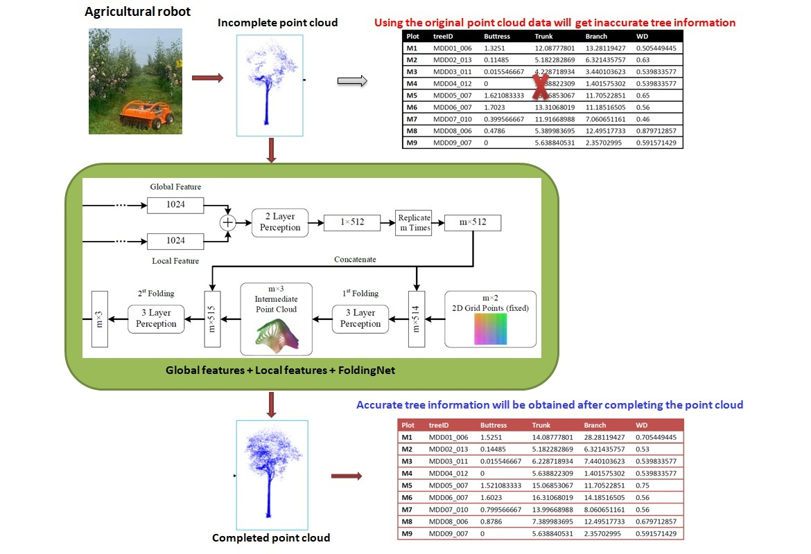
A good point cloud completion method can find clues about global features from partially incomplete point cloud data so as to accurately predict the generation of missing point cloud data. The completed point cloud can be more effectively applied to the modeling and quantitative analysis of the quantitative structure of trees. In order to complete the shape of 3D objects with unordered and unstructured point cloud data, one needs to fully mine the structural information and long-range relationship in the known point cloud. Therefore, the point cloud completion problem can be modeled as a translation problem from one incomplete set to another complete set. Deep learning, an artificial intelligence (AI) method widely used in recent years, has been widely introduced to solve this problem. The existing point cloud completion methods based on deep learning are mainly applied to the point cloud completion of urban scenes and indoor regularized objects, but the research objects generally have obvious continuity and symmetry characteristics. There has been no relevant research on the point cloud completion method for objects with obvious individual morphological differences, such as trees.

The purpose of this work is to provide a method that can complement the point cloud of a single tree. The point cloud of a single tree can be independently collected or obtained from the point cloud of multiple trees. The proposed method firstly uses PointNet, based on point structure, to extract the global features of trees, and then uses EdgeConv, based on graph structure, to extract the local features of trees. After integrating the global and local features, FoldingNet is used to generate a complete point cloud so as to complete the tree point cloud with obvious individual morphological differences. The organizational structure of this paper is as follows. Section 2 describes the latest progress in point cloud completion research using deep learning methods, while Section 3 describes the deep learning model proposed to solve the point cloud completion problem of trees without obvious symmetry characteristics. Section 4 introduces the experimental test and verification results used to verify the effect of tree point cloud completion. Finally, the last section of this paper summarizes the conclusions and future work.

2. Related Work

As an important research direction of machine learning, deep learning has achieved great success in the field of computer vision. After SqueezeNet [15] was proposed, deep learning began to be widely used in image recognition, image segmentation, and image restoration. With the declining cost of 3D data acquisition hardware and the improvement in data acquisition performance, a large number of 3D data have begun to emerge. However, the data collected by 3D devices often cause partial data loss due to occlusion or interference. As the most potential solution in machine vision, deep learning has been widely introduced, moving closer to point cloud data completion. When using a deep learning network to complete a point cloud, it can be divided into two stages: the point cloud feature extraction stage, and the complete point cloud reconstruction stage.

In the feature extraction stage of a point cloud, PointNet [16] introduced max-pooling for the first time to effectively solve the disorder of point cloud data and introduced T-Net to solve the rotation invariance of point cloud data so as to directly extract the features of the original point cloud data. However, this pooled feature extraction method easily loses context information, resulting in an inability to describe structural features in detail. In order to correct this point, PointNet++ [17] added a local area feature extraction module based on the K-neighborhood algorithm to the basic structure of PointNet so as to realize the multi-scale sampling of point cloud data to meet the feature extraction of different local structures. Inspired by the huge success of two-dimensional image convolution calculations, a large number of recent studies have used improved three-dimensional convolution methods to complete feature extraction by extending convolution to irregular coordinate spaces [18,19,20,21,22,23,24]. At the same time, the graph-based method regards the point cloud as a graph structure and the point as a node and uses edges to represent its local connectivity [24,25]. EdgeConv [24] was proposed to deal with k-nearest neighbor nodes and realize the dynamic extraction of local features according to the coordinate distance and semantic affinity. Although these deep learning networks can describe the local structure well, they cannot consider the global shape at the same time.

In the reconstruction phase of a complete point cloud, in order to complete the 3D coordinate points, existing research works have designed a large number of different forms of decoders. Among them, the more representative ones include a decoder based on a multi-layer perceptron [26], decoders based on tree and pyramid multi-level structures [27,28], and a point cloud generator optimized through continuous iteration [29]. A breakthrough research work developed FoldingNet [30], which has provided inspiration for the design of various subsequent generators by guiding the nonlinear folding of 2D meshes to represent 3D point clouds. PCN [31] generates a dense complete point cloud with real structure in the missing area by distributing the use of a full-connection-based decoder and a fold-based decoder at different stages. AtlasNet [32] was proposed as a new method for generating 3D surfaces and completes a point cloud by predicting the position of a group of 2D squares on the point cloud surface. MSN [33] divides the process of point cloud completion into two stages. In the first stage, coarse-grained point cloud completion is achieved in a way similar to AtlasNet. In the second stage, a new sampling algorithm is used to fuse the coarse-grained predicted values with the input point cloud. SA-Net [34] is a hierarchical folding method that can gradually generate detailed spatial structure. SFA-Net [35] does not improve the folding mechanism but solves the problem of information loss in the process of global feature extraction. Recently, SPG [36] comprehensively compared and studied the advantages and disadvantages of various point cloud generators and proposed using a differentiable renderer to project the completed data points onto a depth map and applying a countermeasures network to enhance the perceptual authenticity from different viewpoints.

3. Deep Learning Network Structure

This chapter introduces the proposed method of depth filling a single-tree point cloud based on feature fusion, which can complete the tree point cloud with obvious individual shape differences by solving the local incomplete problem in the filling. The overall network architecture is shown in Figure 1. Section 3.1 first introduces the tree global feature extraction method based on a point-structured PointNet network. Then, in Section 3.2, the local feature extraction method of trees based on an EdgeConv network of a graph structure is introduced. Section 3.3 proposes a FoldingNet point cloud generation network integrating global and local features.

3.1. PointNet-Based Global Feature Extraction Network

In order to better capture the global information of a single point cloud, in this study, the global feature extraction network of PointNet was used for reference, as shown in Figure 2. The network can directly use the 3D coordinates of the point cloud as input.

Due to the rotation invariance of point cloud data, a natural solution is to align all input sets into a standard space before feature extraction. The PointNet-based network introduces a T-Net network to learn the rotation of a point cloud so as to align objects in a space. Jaderberg et al. [37] introduced a spatial converter when aligning 2D images for the first time, and the input form of a point cloud allows for a simpler processing method. This method does not need to introduce a new neural network layer, nor does it need to introduce aliases such as 2D images. In this study, we only needed to design a small network T-Net to predict the affine transformation matrix and apply the transformation directly to the input coordinates for alignment.

$$L_{reg}=\Vert I-A{A}^T\Vert {}_F^2$$

(1)

This idea can be further extended to feature space alignment. In this study, another alignment network was inserted into the point features, and a feature transformation matrix was predicted to align the point cloud features from different inputs, as shown in Formula (1), where A is the feature alignment matrix of a small network prediction. Orthogonal transformation will not lose any input information, and by adding regularization terms, the optimization will become more stable, and the model can obtain a better performance. The network then maps the features of the point cloud to a 64-dimensional space through the shared multi-layer perceptron (MLP). When projecting the features of the point cloud to a higher dimension, in order to maintain rotation invariance, the network again uses T-Net for the alignment after extending the feature space. Finally, the shared MLP is used again to map features to a 1024-dimensional space. At this time, for each point in the point cloud, there is a 1024-dimensional vector representation.

$$f\left(\left\{x_1,x_2,\dots ,x_n\right\}\right)\approx g\left(h\left(x_1\right),h\left(x_2\right),\dots ,h\left(x_n\right)\right)$$

(2)

Another factor that needs to be focused on when extracting the features of point clouds is their disorder. A simple way to maintain disorder is to use symmetric functions, as shown in Formula (2), where h represents the network estimation value of a multi-layer perceptron, and g represents symmetric functions, which commonly include SUM and MAX. After mapping the 3D point cloud to a 1024-dimensional space, in this study, the MAX function was chosen for calculation, which can increase the efficiency of calculation on the basis of minimizing the feature loss. When using this method for the feature extraction of point clouds, the global features of point cloud data sets can be fully preserved.

3.2. EdgeConv-Based Local Feature Extraction Network

PointNet can better extract the global features of point clouds, but it still has shortcomings in extracting local features. In order to improve the accuracy of extracting the local features of point clouds, this study introduced a convolution network based on EdgeConv. EdgeConv [24] is a method that can effectively capture local features. This method maintains the local geometric structure of a point cloud by constructing the adjacent point graph of the point.

Assume that the point cloud has n F-dimension points, which can be expressed as $X=\left\{{\mathrm{x}}_1,\dots ,{\mathrm{x}}_{\mathrm{n}}\right\}\subseteq {ℝ}^F$. In general, $F=3$, and each point can be represented as a 3D coordinate ${\mathrm{x}}_{\mathrm{i}}=\left(x_i,y_i,z_i\right)$. In the architecture of a deep neural network, each subsequent layer operates on the output of the previous layer, where F represents the characteristic dimension of the given layer. The idea of EdgeConv is to construct each point in the point cloud as a directed graph to represent the local point cloud features, which can be expressed as G = (V,E) where V represents the set of K adjacent points of a point, and E represents the edge set of these points and the center point. At this point, EdgeConv defines the edge feature as $e_{ij}=h_{\mathsf{\Theta }}\left({\mathrm{x}}_{\mathrm{i}},{\mathrm{x}}_{\mathrm{j}}\right), \mathrm{where} h_{\mathsf{\Theta }}:{ℝ}^F\times {ℝ}^F\to {ℝ}^{F^{\prime }}$ is a nonlinear function with parameter $\mathsf{\Theta }$. At this point, a new point feature $x_i^{\prime }$ containing local information can be generated by setting the aggregation operation for this group of edge features, as shown in Figure 3. In order to better capture neighborhood information, this study set the h function, as shown in Formula (3).

$$h_{\mathsf{\Theta }}\left({\mathrm{x}}_{\mathrm{i}},{\mathrm{x}}_{\mathrm{j}}\right)={\overline{h}}_{\mathsf{\Theta }}\left({\mathrm{x}}_{\mathrm{i}},{\mathrm{x}}_{\mathrm{j}}-{\mathrm{x}}_{\mathrm{i}}\right)$$

(3)

This makes the local and global features of the point cloud better connected, where ${\mathrm{x}}_{\mathrm{j}}-{\mathrm{x}}_{\mathrm{i}}$ is used to capture neighborhood information, and ${\mathrm{x}}_{\mathrm{i}}$ is used to represent the location of local features in the global. After the point cloud data flow into the network, each point is calculated by the k-NN algorithm using the Euclidean distance in three-dimensional space to calculate the nearest k neighboring points. The aggregation operation used when aggregating features is shown in Formula (4), which can be implemented as a shared MLP. The parameter of the neural network is $\mathsf{\Theta }=\left({\theta }_1,\dots ,{\theta }_M,{\varphi }_1,\dots ,{\varphi }_M\right).$

$$e_{ijm}^{\prime } = ReLU({\theta }_m · ({\mathrm{x}}_{\mathrm{j}}-{\mathrm{x}}_{\mathrm{i}}) + {\varphi }_m · {\mathrm{x}}_{\mathrm{i}})$$

(4)

The local characteristics of each point are shown in Formula (5).

$$x_{im}^{\text{'}}={}_{j:\left(i,j\right)\in E}{}^{max}e{}_{ijm}^{\text{'}}$$

(5)

The network architecture for local feature extraction is shown in Figure 4. In this study, four EdgeConv layers are continuously used to extract geometric features. The four EdgeConv layers used three shared full-connection layers (64, 64, 128, 256), recalculated the neighborhood graph based on the characteristics of each EdgeConv layer, and used a new graph in the next layer. For all EdgeConv layers, the number of adjacent points k was set to 20. Finally, a shared full-connection layer (1024) was used to aggregate the multi-scale features.

3.3. Point Cloud Generation Network Based on Feature Fusion

In the generation network, the global data and local data are fused, and the two-layer perceptron is used to reduce the dimension. Two consecutive three-layer MLPs are used to guide the fixed 2D grid to be transformed into a three-dimensional point cloud that needs to be reconstructed. The overall network structure is shown in Figure 5. The network copies the fused feature vector m times, and the size is an m × 512 matrix. The matrix is compared with the fixed 2D grid’s m × 2 matrix connection, splicing m × 514. The output size of the matrix is m after being processed by a three-layer perceptron × 3. After that, the copied feature vector is connected to the output matrix again, and sent to the second three-layer perceptron, which outputs the final reconstructed point cloud.

In FoldingNet, the process of connecting the copied feature matrix to low-dimensional grid points and then conducting MLP point by point is called the folding operation. The folding operation process is equivalent to the mapping process of guiding a general 2D mesh to a 3D point cloud. In order to intuitively understand the folding operation, the input 2D mesh points can be represented by a matrix U, where $u_i$ is the ith row of the matrix U, and each row is a two-dimensional grid point. M represents the fused feature vector. After splicing it with the row i of the matrix U, the row i of the input matrix of MLP can be expressed as $\left[u_i,\theta \right]$. Since MLP is applied to each row of the input matrix in parallel, the row i of the output matrix can be written as $f\left(\left[u_i,\theta \right]\right)$, where f represents the function constructed by MLP. The function can be regarded as a parameterized high-dimensional function, and the eigenvector θ is used as the parameter to guide the function structure (folding operation).

Because MLPs are good at approximating nonlinear functions, they can perform fine folding operations on 2D meshes. The high-dimensional feature matrix essentially stores the force required for folding, which makes the folding operation more diversified. The generator uses two consecutive collapse operations. The first is to fold 2D meshes into a 3D space, and the second is to carry out more refined folding inside the 3D space. Each folding operation has a relatively simple operation. The combination of the two folding operations can produce a fairly fine surface shape. Although the first folding seems simpler than the second, they together produce substantial changes in the final output. If a finer surface shape is needed, more successive folding operations can be applied.

4. Experimental Evaluation

4.1. Computing Platform and Test Environment

In order to verify the effectiveness of the single-tree point cloud completion method based on feature fusion proposed in this paper, this study used PyTorchto develop the neural network model described above. In order to quickly complete the pre-training of the multi-agent reinforcement learning model, in this step, the server was used as the training node, and the GPU graphics card was used to accelerate the training of the neural network. The hardware and software configuration of the server is shown in

Table 1. Hardware configuration.

Hardware	Configuration
Processor	Intel(R) Xeon(R) Gold 6278C CPU @ 2.60GHz * 2
Graphics card	NVIDIA GeForce RTX 3090 * 2
Memory	128 GB
Disk	2TB * 2 HDD

and

Table 2. Software configuration.

Software	Version
Operating system	Ubuntu 20.04
GPU driver	460.32.03
CUDA library	11.2
Python	3.9.1
PyTorch	1.9.0 + cu111

.

4.2. Experimental Data

In this study, the tree data set collected by Wageningen University in the Netherlands was used. The data set is composed of 29 single-tree TLS point clouds, destructive sampling data, and forest survey data. The tree point cloud was generated by RIEGL VZ-400 3D^® and collected by a ground laser scanner. For the detailed configuration of the tree selection and scanner, please refer to paper [38], published earlier. The paper also provides the destructive geometric measurement data of 29 trees from Peru, Indonesia, and Guyana. The data cover the sample plot number, tree number, and tree species name, as well as the geometric size, DBH, tree height, and wood basic density of different parts of each tree, the main information is given in

Table 3. Study site descriptions [38].

	Peruvian Site	Indonesian Site	Guyanese Site
Number of plots	9	10	10
Forest type	Lowland tropical moist terra firme forest	Peat swamp forest	Lowland tropical moist forest
Region	Madre de Dios. Southwestern Amazon	Mentaya River (Central Kalimantan)	Vaitarna Holding’s concession
Lat/long	−12.27 lat −69.10 long	−2.41 lat 113.13 long	6.04 lat −58.70 long
Mean elevation	312 m a.s.l.	22 m a.s.l.	117 m a.s.l.
Mean stem density (trees with diameter at breast height (DBH) > 10 cm)	565 stems/ha	1314 stems/ha	516 stems/ha
Mean DBH harvested trees (SD)	90.0 cm (22.2 cm)	58.4 cm (18.2 cm)	73.7 cm (12.0 cm)

and

Table 4. Terrestrial laser scanning specifications [38].

Equipment Specifications	Value
Wavelength	1550 nm
Beam divergence	0.35 mrad
Scan range	360° in azimuth 100° in zenith
Scan resolution	0.06°

.

This study selected the data of 29 trees as the complete point cloud data set. In order to reduce the amount of computation, the data of the point cloud were down-sampled to 30,000 data points, and the method in the study by [31] was used to convert it into a missing point cloud data set so that each tree generated 2000 incomplete point clouds, 23 trees were randomly selected as the training data set, and the remaining 6 trees were used as the test data set. In the training process, the number of iterations (epoch) of the neural network was 150, the batch size was 32, the parameter optimizer was Adam, and the learning rate decreased by 0.1 per 100 cycles. The computing platform in Table 1 and Table 2 was used to collect the training and test data.

4.3. Loss Function

Because point clouds are unordered, it is necessary to maintain the invariance of point arrangement when determining the similarity of point clouds. Chamfer Distance (CD) [39] and Earth Mover’s Distance (EMD) [33] are commonly used to measure the distance between two point clouds. The lower the values of these two distances, the higher the similarity of the two point clouds. Therefore, a large number of studies have designed loss functions based on these two distances to train the parameters of neural networks.

$${\mathrm{d}}_{\mathrm{CD}}\left({\mathrm{S}}_1,{\mathrm{S}}_2\right)=\frac{1}{\left|{\mathrm{S}}_1\right|}{\displaystyle \sum }_{\mathrm{x}\in {\mathrm{S}}_1}{}_{\mathrm{y}\in {\mathrm{s}}_2}{}^{\min }\Vert \mathrm{x}-{\mathrm{y}\Vert }_2^2+\frac{1}{\left|{\mathrm{S}}_2\right|}{\displaystyle \sum }_{\mathrm{x}\in {\mathrm{S}}_2}{}_{\mathrm{y}\in {\mathrm{s}}_1}{}^{\min }\Vert \mathrm{x}-{\mathrm{y}\Vert }_2^2$$

(6)

$${\mathrm{d}}_{\mathrm{EMD}}\left({\mathrm{S}}_1,{\mathrm{S}}_2\right)=\underset{\varnothing :{\mathrm{S}}_1\to {\mathrm{S}}_2}{\min }\frac{1}{\left|{\mathrm{S}}_1\right|}{\displaystyle \sum }_{\mathrm{x}\in {\mathrm{S}}_1}\Vert \mathrm{x}-\varnothing {\left(\mathrm{x}\right)\Vert }_2$$

(7)

In Formula (6), ${\mathrm{d}}_{\mathrm{CD}}$ represents the chamfer distance between two point clouds, and d_EMD in Formula (7) represents the moving distance between two point clouds. ${\mathrm{S}}_1 \mathrm{and} {\mathrm{S}}_2$ represent the two different point clouds to be compared, and $\mathrm{x}$ and $\mathrm{y}$ represent the points in ${\mathrm{S}}_1$ and ${\mathrm{S}}_2$ respectively. $\varnothing :{\mathrm{S}}_1\to {\mathrm{S}}_2$ represents the bijection of the set, and $\varnothing \left(\mathrm{x}\right)$ represents the point uniquely corresponding to x in ${\mathrm{S}}_2$.

The EMD calculation process of these two distances is relatively complex, but the distance between the best matching points of the two different point clouds can be calculated. However, although the computational complexity of the CD is relatively low, it can only calculate the average distance between the closest points of two different point clouds.

$$\mathrm{Loss}\left({\mathrm{Y}}_{\mathrm{intermediate}},{\mathrm{Y}}_{\mathrm{final}},{\mathrm{Y}}_{\mathrm{gt}}\right)={\mathrm{d}}_{\mathrm{CD}}\left({\mathrm{Y}}_{\mathrm{intermediate}},{\mathrm{Y}}_{\mathrm{gt}}\right)+{\mathsf{\alpha }\mathrm{d}}_{\mathrm{EMD}}\left({\mathrm{Y}}_{\mathrm{final}},{\mathrm{Y}}_{\mathrm{gt}}\right)$$

(8)

When using FoldingNet for folding, this study used two consecutive folding operations. The first fold operation outputs the middle point cloud ${\mathrm{Y}}_{\mathrm{intermediate}}$, and the second outputs the final result ${\mathrm{Y}}_{\mathrm{final}.}$ Therefore, this study used the combination of CD and EMD to construct the loss function. First, the CD was used to evaluate the distance between the intermediate point cloud and the complete (ground truth, gt) point cloud, and the EMD was used to evaluate the distance between the complete point cloud and the final point cloud. The calculation process of the loss function used in the network model in this study is shown in Formula (8).

4.4. Accuracy Comparison between Different Models

In order to highlight the effectiveness of the method in this study, FoldingNet [30], PCN [31], AtlasNet [32], SPG [36], and the method in this study were used to carry out the network training and precision evaluation of point cloud completion for tree data sets. After the point cloud completion network training converged, a group of incomplete point cloud completion data was selected randomly from six trees in the data set for visualization, and the results are shown in Figure 6.

It can be intuitively seen in Figure 6 that the method proposed in this paper was the closest to the original point cloud after completing the incomplete tree point cloud. The SPG method was close to this method. The point cloud completion effects of the FoldingNet and PCN algorithms were relatively poor.

In order to evaluate the effect of point cloud completion more objectively and quantitatively, this study used two widely used point cloud similarity evaluation indicators, CD and EMD. FoldingNet [30], PCN [31], AtalasNet [32], SPG [36], and the method in this paper were used to carry out the network training of point cloud completion on the tree data set. Then each tree was evaluated as a unit, the data were collected, and a histogram was drawn, as shown in Figure 7 and Figure 8. In the figures, the ordinate represents the distance between the CD and the EMD, the abscissa represents the point clouds of different numbers of trees, and the columns of different colors represent different point cloud completion models.

It can be seen in Figure 7 and Figure 8 that the point cloud completion effects of different trees were not the same, which was caused by the different number of data points of point clouds of different trees in the data set and the different shapes of the trees. According to the CD and EMD indexes, the method proposed in this paper had the lowest distance from the original point cloud and the highest point cloud completion accuracy. The SPG method also had an advantageous position from the average value, but it was slightly inferior to the method in this paper. The distance between the point cloud and the original point cloud after the completion of the FoldingNet and PCN algorithms was significantly higher than that of other algorithms, indicating that the completion effect was relatively weak, which is consistent with the analysis conclusion of intuitive comparison in Figure 6. According to the analysis of all the data, this method was superior to the previous work according to the CD and EMD indicators. Taking the minimum value of the distance in the other four models as a reference, the method in this paper had an average increase of 21.772% in the CD index compared to the optimal model. Taking the minimum value of the distance in the other four models as a reference, the EMD index of this method was 15.672% higher than that of the optimal model on average. Thus, this effectively proves that the method in this paper was superior to the other methods in point cloud completion accuracy.

4.5. Comparison of Modeling Accuracy of Single Timber Quantitative Structure

In order to verify the supporting effect of point cloud complement on the three-dimensional geometric structure reconstruction of a single tree, this study used the tree data set collected by the University of Wageningen in the Netherlands [39] and used the AdQSM model as the tree quantitative structure calculation model [40] to conduct quantitative analysis on the original complete point cloud and the point cloud after using FoldingNet [30], PCN [31], AtalasNet [32], SPG [36], and the method of this paper. Select indicators sensitive to occlusion and missing point clouds were used to evaluate the accuracy of the point cloud completion. The indicators selected in this study were as follows: BranchVolume (BV), BranchesNum (BN), and BranchesSurfaceArea (BSA). The evaluation formula for accuracy is shown in (9).

$$F_{accuracy}=\frac{\left|B{V}_{pt}-B{V}_{gt}\right|}{B{V}_{gt}}+\frac{\left|B{N}_{pt}-B{N}_{gt}\right|}{B{N}_{gt}}+\frac{\left|BS{A}_{pt}-BS{A}_{gt}\right|}{BS{A}_{gt}}$$

(9)

When using AdQSM modeling, there are two relatively important parameters, height segmentation (HS) and cloud parameter (CP), which were set to 0.50 and 0.003, respectively, in this study. The statistical data were analyzed and plotted, as shown in Figure 9. Among them, the ordinate represents the 3D reconstruction accuracy of a single tree, the abscissa represents the point cloud of different numbers of trees, and the columns of different colors represent different point cloud completion models.

It can be seen in Figure 9 that the quantitative analysis accuracy of different trees after point cloud completion was not consistent, which was caused by the different number of data points of different tree point clouds in the data set and the different shapes of the trees. From all the data, the method in this paper was superior to the previous works in terms of the $F_{accuracy}$ index. Taking the minimum accuracy of the other four models as a reference, the method in this paper had an average improvement of 37.61% compared to the optimal model in terms of the $F_{accuracy}$ index. This effectively proves that the method in this paper can better support the reconstruction of a 3D geometric structure of a single tree.

4.6. Analysis of Time Cost of the Model

In order to use the point cloud completion method proposed in this paper in agricultural robots and process incomplete point cloud data in real time, it is necessary to introduce a GPU accelerator card to accelerate the neural network model. Nvidia has produced a number of devices suitable for Internet of Things solutions in its Jetson series of equipment products. These include the powerful 512-core Jetson AGX Xavier, the mid-range 256-core Jetson TX2, and the entry-level $99 128-core Jetson Nano. At the same time, Nvidia also provides TensorRT for high-performance deep learning reasoning, which can provide low latency and high throughput for deep learning applications, and its performance is nearly 40 times faster than that of the pure CPU platform. This study selected the entry-level Jetson Nano to complete the real-time processing of residual and defective cloud data. PyTorch, used in this study, can easily complete the training of in-depth learning and point cloud completion with TensorRT.

As can be seen in Figure 10, for network models with different complexity, the speed of processing point cloud data is not the same after training convergence. Among them, FoldingNet and Atlas Net have relatively simple network structures and relatively fast processing speeds. The model structures of PCN and the method in this paper are relatively complex, and the speeds are relatively slow when processing point cloud data. However, the processing times of all models do not exceed 120ms, so the real-time processing requirements can be met when processing point cloud data sets, and the impact of model complexity can be ignored.

5. Conclusions

Regarding the visual perception of agricultural robots, this work introduces a method of using a depth learning model to complete laser point clouds of trees acquired by mobile robots. This method can be used not only to process the point cloud data obtained by scanning a single tree but also to complete the point cloud of a single tree separated from a piece of trees. The paper describes the methods used in the study, the evaluation indicators that prove the effectiveness of the study, and the data used in the evaluation. The experiment shows that this method had obvious advantages in many evaluation indexes. At the same time, the applicability of this method on the agricultural robot platform is illustrated by the calculation time analysis on the common mobile computing platform.

This method not only effectively explores the accurate acquisition of tree point clouds but also provides a good solution for the completion of irregular object point cloud data. However, it should also be noted that this method was only developed for the completion of the point cloud of a single tree. It will be more valuable if it can complete the point cloud of a whole row of trees, which will be an important focus of future work.