A New Hybrid Fault Diagnosis Method for Wind Energy Converters

Abstract

Fault diagnostic techniques can reduce the requirements for the experience of maintenance crews, accelerate maintenance speed, reduce maintenance cost, and increase electric energy production profitability. In this paper, a new hybrid fault diagnosis method based on multivariate empirical mode decomposition (MEMD), fuzzy entropy (FE), and an artificial fish swarm algorithm (AFSA)-support vector machine (SVM) is proposed to identify the faults of a wind energy converter. Firstly, the measured three-phase output voltage signals are processed by MEMD to obtain three sets of intrinsic mode functions (IMFs). The multi-scale analysis tool MEMD is used to extract the common modes matching the timescale. It studies the multi-scale relationship between three-phase voltages, realizes their synchronous analysis, and ensures that the number and frequency of the modes match and align. Then, FE is calculated to describe the IMFs’ complexity, and the IMFs-FE information is taken as fault feature to increase the robustness to working conditions and noise. Finally, the AFSA algorithm is used to optimize SVM parameters, solving the difficulty in selecting the penalty factor and radial basis function kernel. The effectiveness of the proposed method is verified in a simulated wind energy system, and the results show that the diagnostic accuracy for 22 fault modes is 98.7% under different wind speeds, and the average accuracy of 30 running can be maintained above 84% for different noise levels. The maximum, minimum, average, and standard deviation are provided to prove the robust and stable performance. Compared with the other methods, the proposed hybrid method shows excellent performance in terms of high accuracy, strong robustness, and computational efficiency.

1. Introduction

1.1. Background

Wind power systems are supposed to be a sustainable solution to satisfy the increasing energy demand and alleviate the impact of greenhouse gas emissions [1]. High reliability and low maintenance cost are the key to the large-scale development of wind power systems [2,3]. Fault diagnosis is considered as a powerful tool to ensure good operation of the systems, reduce downtime, and improve maintenance efficiency [4,5].

The converter is an indispensable component in a wind power system. The high annual failure rate of 17.5% and downtime percentage of 14.3% indicate that the wind energy converter is vulnerable [6]. Its failure will lead to the increase in harmonics, which can reduce power quality. Its failure will also damage other important components in the system, thus increasing production costs, and even endangering the security of the power grid [7]. Therefore, it is necessary to diagnose the faults of wind energy converters.

1.2. A Survey of Previous Related Work

The model-based method uses the physical knowledge of system structure and dynamics to establish an accurate analysis model for the converter system, and then obtains the fault results by analyzing the residual between the estimation and the actual measurement. A sliding mode observer-based robust fault diagnosis method was proposed for a closed-loop grid-connected inverter [8]. A Kalman filter estimation method was used to directly and quickly detect the fault submodule of modular multilevel converter [9]. These methods can observe the essential fault characteristics of the system and make full use of system information; they are conducive to finding early-stage weak faults. However, the diagnostic accuracy of these methods deeply depends on the accuracy of system parameters and models.

The signal-based method detects and locates converter faults by comparing diagnostic variables and thresholds. The absolute normalized current was calculated to diagnose the open-circuit faults of the converter in a wind turbine [10]. A fault diagnosis strategy based on current trajectory was used for a wind power converter [11]. These methods are simple and straightforward because they do not need a precise converter system model, and they have significant real-time performance. However, they require prior knowledge of the system and are susceptible to threshold. Moreover, the diagnostic accuracy is sensitive to noise and operating conditions.

The data-driven method overcomes the defects of the above methods; it does not need an accurate converter model or prior system knowledge. This method uses mathematical technology to diagnose converter faults, and only requires a large amount of data. Wang extracted the fast Fourier transform (FFT)-principal component analysis (PCA) features of a converter signal to construct the fault feature vector, and identified faults through a multiclass relevance vector machine (mRVM) [12]. FFT-relative principal component analysis (RPCA) was proposed to extract generator-side converter fault features, and a support vector machine (SVM) was used for fault type recognition [13]. The FFT-PCA-Bayes networks (BNs) integration method was presented for inverter fault diagnosis to solve the uncertainty caused by bias and noise of sensors [14]. The discrete wavelet transform (DWT) was used to preprocess inverter current to obtain approximate coefficients, and then their energy vectors were calculated as fault features [15]. DWT was utilized to extract detail coefficients as fault features, and an artificial neural network (ANN) was used to recognize inverter switch faults [16]. The energy of each layer wavelet transform (WT) coefficient was extracted as fault features, and then input into the deep belief networks (DBN) model for fault classification [17]. However, for non-stationary and nonlinear wind energy converter signals, FFT and DWT are unable to guarantee the accuracy of fault diagnosis. This is because FFT generates error information for nonlinear signals and has no time resolution, and DWT is easily affected by wavelet bases and lacks adaptability.

According to the characteristics of the signal itself, empirical mode decomposition (EMD) adaptively decomposes a non-stationary and nonlinear signal into a set of intrinsic mode functions (IMFs) reflecting signal frequency, which overcomes the defects of FFT and DWT [18]. EMD was combined with PCA to extract fault features for converter fault diagnosis, and SVM was used as classification model [19]. In order to improve noise robustness, a fault diagnosis method based on ensemble EMD (EEMD), norm entropy (NE), and SVM was proposed, and the fault features were described by IMF-NE [20]. Complete EEMD (CEEMD) was used to detect the harmonic characteristics of the three-stator currents and the feature was input ANN for converter fault diagnosis [21]. However, these methods have limitations in processing multi-channel signals; each channel signal needs to be decomposed separately, which may lead to different IMF quantities finally obtained, or inconsistency in the corresponding frequency of IMF of the same order [22].

In addition, although SVM has good processing ability for small samples and nonlinear data, its parameters penalty coefficient and kernel function can affect the accuracy of fault diagnosis [23]. They cannot be selected adaptively according to actual samples, leading to low accuracy of classification and slow convergence [24]. Grid search and cross-validation (CV) were used to determine the optimal values of penalty coefficient and kernel function [20]. The average value of three-phase current was taken as the fault feature and input into the SVM classifier optimized by a genetic algorithm (GA), then the power switch faults of the converter were effectively detected and located [25]. An intelligent detection algorithm combining variational mode decomposition and particle swarm optimization (PSO) SVM was proposed, which can not only accurately identify the series arc fault in a solar photovoltaic power generation system, but can also identify the parallel arc fault [26]. A fault identification method based on cuckoo search (CS)-SVM was proposed to monitor the status of wind turbines, and the CS algorithm was used to select the optimal SVM parameters [27]. These methods improve the accuracy of fault diagnosis, but increase the calculation cost.

In order to clarify the advantages of the presented hybrid fault diagnosis method for wind energy converters with other algorithms previously published, a comparison is made, as shown in

Table 1. Comparison of converter fault diagnosis methods.

Ref.	Approach	Method	Advantage	Drawback
[8,9]	Sliding mode observer [8]; Kalman filter estimation method [9]	Model-based	1. Observe the essential fault characteristics of the system; 2. Make full use of system information; 3. Conducive to finding early-stage weak faults.	Heavily depends on the accuracy of system parameters and models
[10,11]	Absolute normalized current [10]; Current trajectory [11]	Signal-based	1. Simple and straightforward; 2. Significant real-time performance	1. Requires prior-knowledge of the system; 2. Susceptible to threshold; 3. Sensitive to noise and operating conditions.
[12,13,14,15,16,17]	FFT-PCA-RVM [12]; FFT-RPCA-SVM [13]; FFT-PCA- BNs [14]; WT-energy vectors [15]; DWT-detail coefficients-ANN [16]; WT-energy vectors-DBN [17]	Data-driven	1. Does not need accurate model; 2. Does not need system prior knowledge.	1. FFT generates error information for nonlinear signals; 2. FFT has no time resolution; 3. DWT is easily affected by wavelet bases and lacks adaptability; 4. Detail coefficients, energy vectors, and principal component energy are sensitive to load, the changing operating conditions, and noise; 5. ANN: needs a large number of samples, heavily relies on learning samples, easy to fall into local optimum; 6. DBN: Heavy complexity and calculation.
[19,20,21]	EMD-PCA-SVM [19]; EEMD-NE-SVM [20]; CEEMD-ANN [21]	Data-driven	1. Nonlinear signal processing; 2. Adaptive signal processing; 3. SVM: suitable for a small number of samples, simple/straightforward, high generalization ability, with global optimality.	1. Have limitations in processing multi-channel signals; 2. ANN: needs a large number of samples, heavily relies on learning samples, easy to fall into local optimum; 3. SVM: difficulty in selecting the penalty factor and radial basis kernel parameter in SVM model.
[20,25,26,27]	CV-SVM [20]; GA-SVM [25]; PSO-SVM [26]; CS-SVM [27]	Data-driven	Improve the diagnostic accuracy	Increase the calculation cost

.

1.3. Motivation

Since the power of the wind energy converter is continuously increasing, and the actual working conditions are very complex and harsh, it is necessary to develop a fault diagnosis method that is easy to transplant, does not need an accurate converter model, and does not need prior knowledge of the signal pattern; moreover, an adaptive fault diagnosis method that is robust enough to withstand noise and changes in operating conditions is also necessary.

As summarized in Table 1, the model dependence of the model-based method and the environmental sensitivity of the signal-based method hinder their application in increasingly complex wind power systems. On the other hand, EMD stands out in signal analysis due to its nonlinear signal processing ability and adaptability. Multi-scale signal analysis is a promising method to improve the accuracy and robustness of diagnosis. It should be noted that feature descriptions such as detail coefficients [16], root mean square [28], energy vector [15], mean [29], standard deviation [30], kurtosis [31], and skewness [32] are sensitive to different working conditions, load disturbance, and noise. Entropy represents the statistical complexity of signals, and can describe the system internal information. Thus, entropy can be used as quantitative description of information contained in signals and quantitative evaluation of system complexity.

This paper presents a multi-scale signal analysis-based hybrid fault diagnosis method for wind energy converters. It combines multivariate empirical mode decomposition (MEMD) and fuzzy entropy (FE) to extract converter fault features, and uses a support vector machine (SVM) optimized by the artificial fish swarm algorithm (AFSA) to identify fault types. Three-phase voltage signals are selected for converter fault diagnosis. Firstly, they are processed using MEMD to obtain three sets of intrinsic mode functions (IMFs), and the same characteristic frequency appears in the same order in different IMF sets. Next, the FE is used to characterize the IMFs’ complexity, and the IMFs-FE value is taken as the fault feature vector. Finally, AFSA is used to optimize the penalty factor and radial basis kernel parameter in the SVM model, and the optimized classifier is used for converter fault identification. The effectiveness of the presented method is verified in a simulated wind energy system, and its robustness is tested. The main contributions are as follows:

• The multi-scale analysis tool MEMD is used to extract the common modes matching the timescale. It studies the multi-scale relationship between three-phase voltages, realizes the synchronous analysis of three-phase voltages, and ensures that the number and frequency of the extract modes match and align;
• IMFs-FE reflects the complexity of intrinsic oscillations, increasing the robustness to operating conditions and noise;
• The best, average, and worst results, and the standard deviations are reported to prove the robust and stable performance;
• The hybrid method shows outstanding performance in terms of high diagnosis accuracy, strong robustness, and high computational efficiency.

The rest of this paper is organized as follows. Section 2 describes a wind energy converter system and analyzes the fault modes. Section 3 presents an intelligent fault diagnosis method, MEMD-FE-AFSA-SVM. Section 4 verifies the effectiveness and robustness of the method in a simulated model. Section 5 provides conclusions.

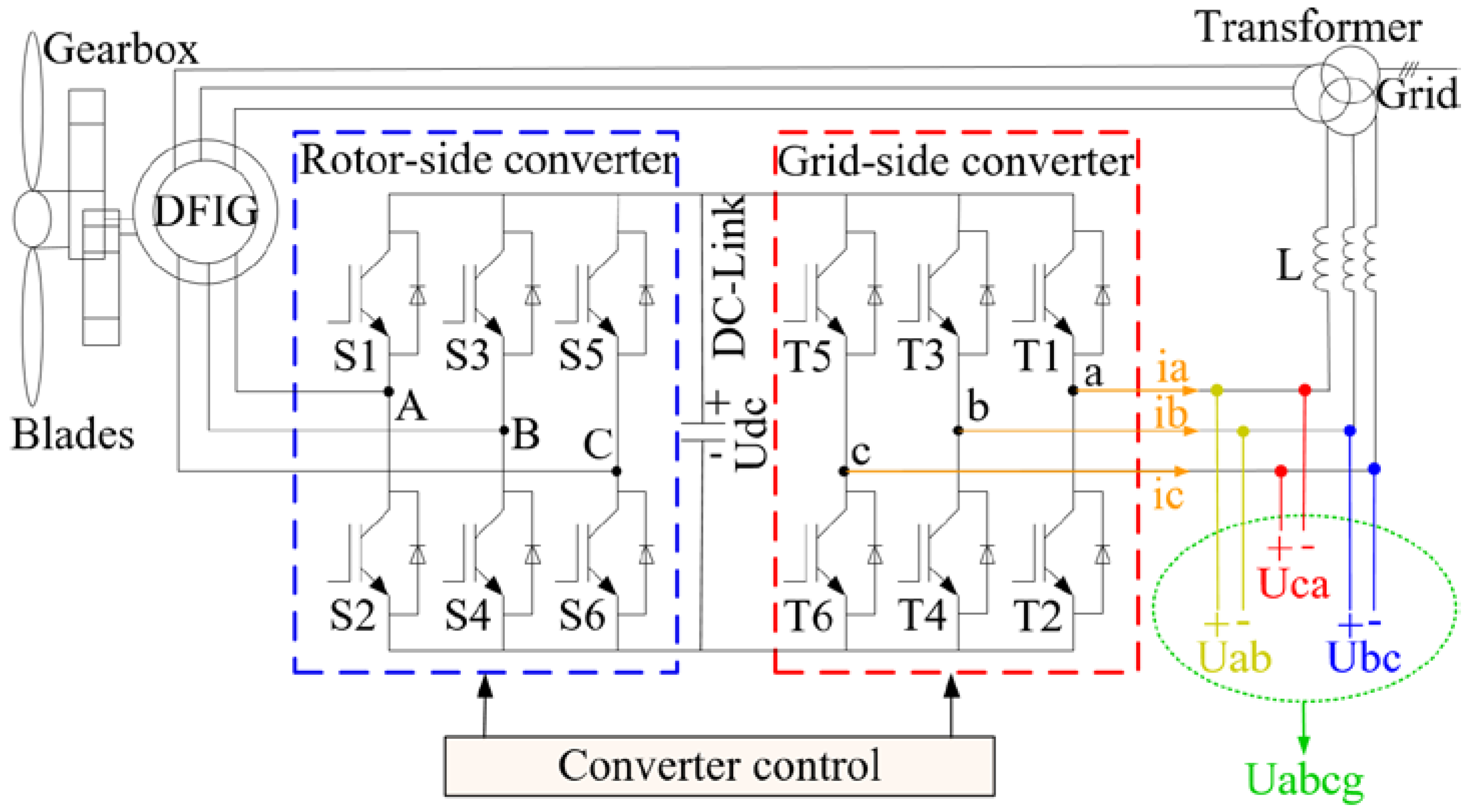
2. Fault Diagnosis System

2.1. System Description

A doubly fed induction generator (DFIG) wind power generation system is shown in Figure 1. It is mainly composed of a converter, control system, generator, blades, and gearbox. The converter converts the alternating current (variable frequency and amplitude) from the generator into constant-frequency alternating current, and it adopts a back-to-back structure. The converter near the grid is called the grid-side converter. It suppresses the current harmonics and stabilizes the DC-link voltage. The converter near the generator is called the rotor-side converter. It tracks the maximum wind energy and improves the system operation efficiency. The grid-side converter and the rotor-side converter have the same structure. The grid-side converter has three bridge arms, and each arm is composed of two insulated gate bipolar transistors (IGBTs). Each IGBT (i.e., Ti) is driven by a gate signal; it is turned off when the signal is 0, and it is turned on when the signal is 1.

Converter faults mainly include open-circuit (OC) faults and short-circuit (SC) faults. The SC fault can generate abnormal overcurrent, which will trigger system protection and cause immediate shutdown, so it is easy to detect. The OC fault will cause current offset in healthy phase and fault phase, leading to generator torque oscillation, and it will also cause high current harmonics, which will reduce the power factor of the grid. Furthermore, it may damage the capacitor and generator. However, OC faults are usually slow to respond and do not result in an immediate shutdown of the system. Therefore, OC fault diagnosis is necessary to reduce operational risk and improve power production.

Selecting the fit signal is the first task of intelligent fault diagnosis. Due to the characteristic that the output voltage of the converter is not affected by the change in load, while the current varies, the three-phase line-to-line voltage U_abcg (U_ab, U_bc, U_ca) is adopted as the input signal of the fault diagnosis model. The simulated voltages U_abcg (U_ab, U_bc, U_ca) under different faults are shown in Figure 2.

From Figure 2, OC faults cause signal distortion in U_ab, U_bc, and U_ca, and the degree of distortion varies with different faults. Therefore, the variation in U_ab, U_bc, and U_ca can reflect the fault state of the converter, and it is reasonable to use them as diagnostic signals to identify the fault type of the converter.

The complex and changeable operating conditions of wind power systems make the output signals of the converter nonlinear and non-stationary, thus, the fault diagnosis method for the converter should have superior processing capability for nonlinear and non-stationary signals. The high dynamics of wind power systems cause abrupt changes in torque, so the converter fault diagnosis should be robust enough to withstand wind speed. Since the signals measured by sensors contain noise, the fault diagnosis method should have robustness to withstand noise.

2.2. Fault Types

Different combinations of IGBT open circuits form different fault types. For the grid-side converter, when all IGBTs are working healthily, the converter is in normal state. When only one IGBT fails, six fault modes are formed: T1, T2, T3, T4, T5, and T6. When two IGBTs in the same half-bridge fail at the same time, six fault modes are formed: T1 and T5, T1 and T3, T3 and T5, T2 and T6, T2 and T4, T4 and T6. When two IGBTs in the same bridge arm are faulty simultaneously, three fault modes are formed: T1 and T2, T3 and T4, T5 and T6. When two IGBTs in different half-bridges fail at the same time, six fault modes are formed: T1 and T6, T1 and T4, T3 and T6, T3 and T2, T5 and T4, T5 and T2. It is rare that OC faults occur in three or more IGBTs simultaneously, so the OC fault diagnosis of single IGBT faults and double IGBTs faults is studied in this work. Thus, there are a total of 22 fault modes in both the faulty and healthy state.

3. Fault Diagnosis Method

3.1. The Proposed Fault Diagnosis Method

The fault diagnosis steps of wind energy converters proposed in this paper include fault feature extraction, classification diagnosis model, and diagnostic results output. The detailed fault diagnosis process is as follows.

Step 1. Acquire the three-phase voltage signal U_abcg (U_ab, U_bc, U_ca) of the converter under different working conditions and take them as input to train and test the fault diagnosis model.

Step 2. Process three fault signals U_ab, U_bc, and U_ca synchronously using MEMD, and three sets of IMFs with matching and aligned number and frequency are obtained.

Step 3. Calculate the FE features of IMFs, and take them as fault features. Then, the fault feature of a sample is obtained as follows.

$$H_{FE}=[H_{FE}(\mathrm{IMFs}{/}_{U_{\mathrm{ab}}}),H_{FE}(\mathrm{IMFs}{/}_{U_{\mathrm{bc}}}),H_{FE}(\mathrm{IMFs}{/}_{U_{\mathrm{ca}}})]$$

where

$$\begin{array}{l}{H}_{FE}(\mathrm{IMFs}{/}_{U_{\mathrm{ab}}})=[H_{FE}(\mathrm{IMF1}{/}_{U_{\mathrm{ab}}}),H_{FE}(\mathrm{IMF2}{/}_{U_{\mathrm{ab}}}),\dots ,H_{FE}(\mathrm{IMF}l{/}_{U_{\mathrm{ab}}})]\\ H_{FE}(\mathrm{IMFs}{/}_{U_{\mathrm{bc}}})=[H_{FE}(\mathrm{IMF1}{/}_{U_{\mathrm{bc}}}),H_{FE}(\mathrm{IMF2}{/}_{U_{\mathrm{bc}}}),\dots ,H_{FE}(\mathrm{IMF}l{/}_{U_{\mathrm{bc}}})]\\ H_{FE}(\mathrm{IMFs}{/}_{U_{\mathrm{ca}}})=[H_{FE}(\mathrm{IMF1}{/}_{U_{\mathrm{ca}}}),H_{FE}(\mathrm{IMF2}{/}_{U_{\mathrm{ca}}}),\dots ,H_{FE}(\mathrm{IMF}l{/}_{U_{\mathrm{ca}}})]\end{array}$$

l is the number of IMF in each set.

Step 4. The fault features are divided into training samples and test samples. The training samples are used to train the SVM classification model, and the test samples are used to validate the diagnostic performance.

Step 5. Train SVM classification model and output diagnostic results. The SVM model is optimized by a swarm intelligence algorithm AFSA to obtain the best model parameters.

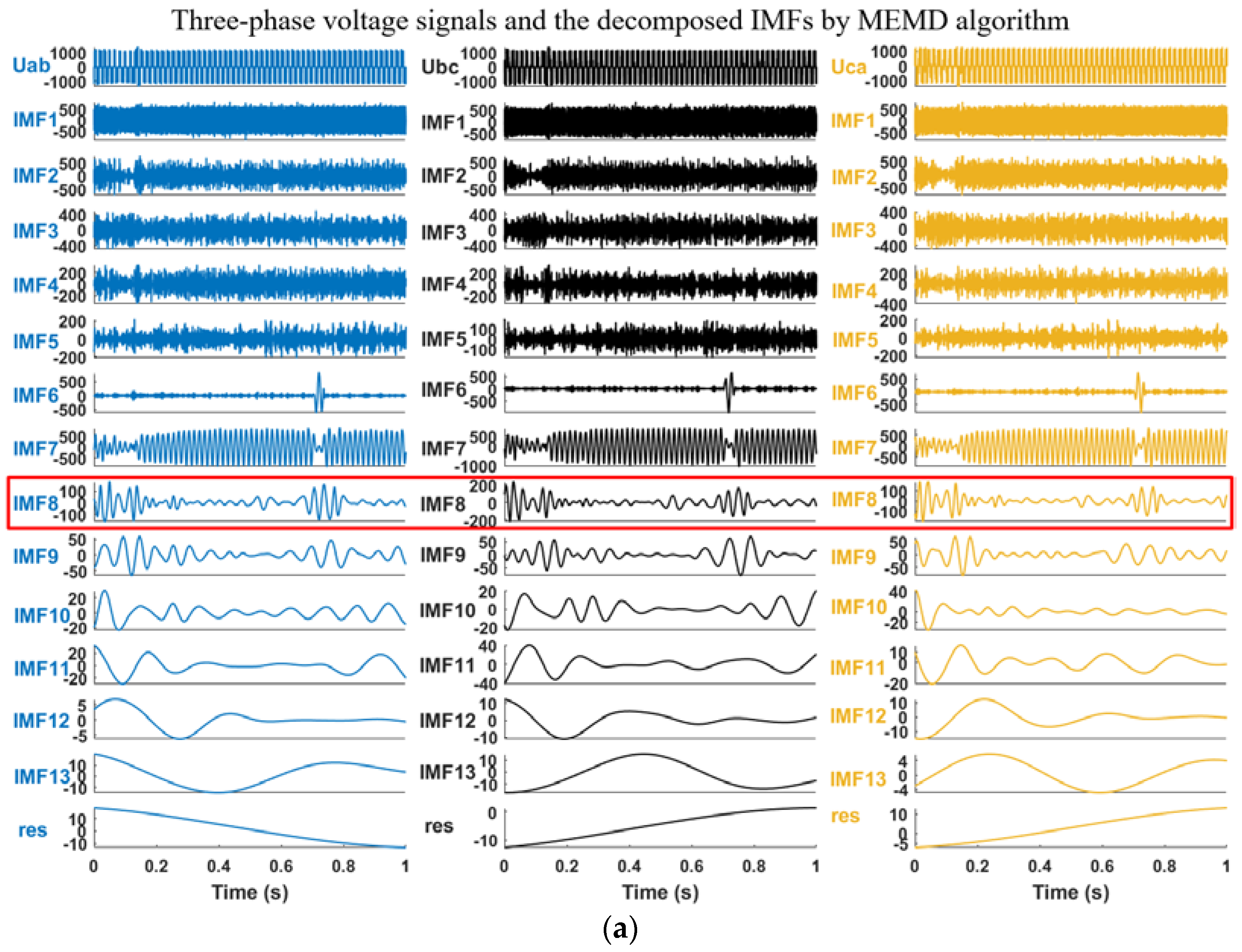
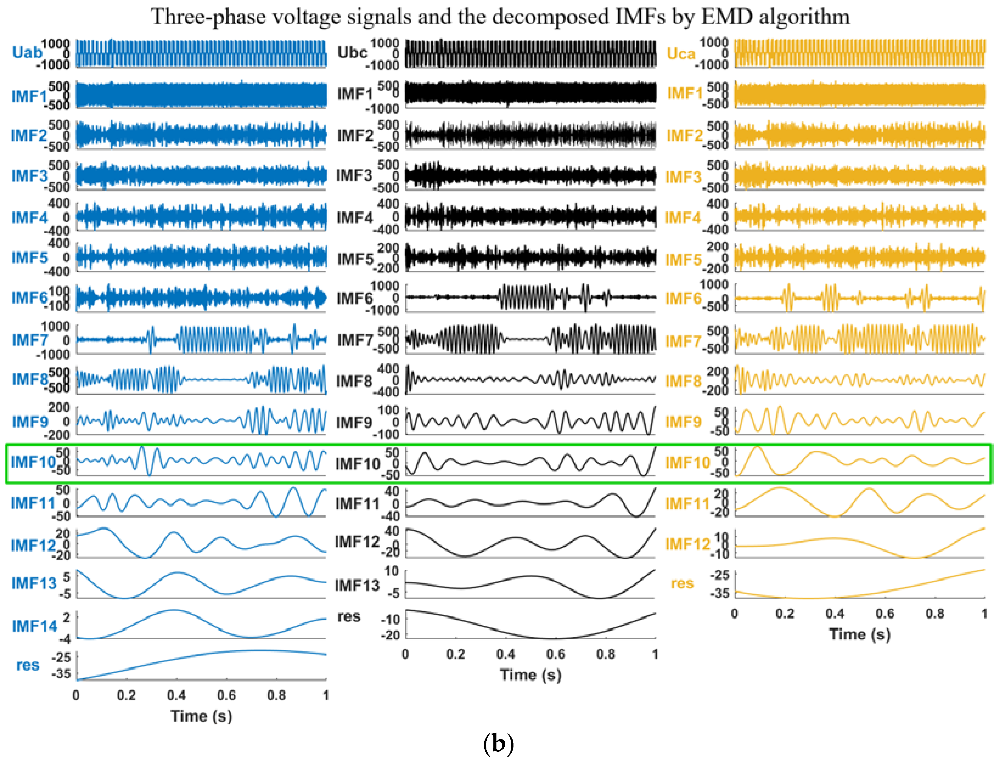
3.2. Signal Decomposition Using MEMD

Multivariate empirical mode decomposition (MEMD) extends EMD to multivariate signal processing [33]. MEMD projects multi-dimensional signals to the direction vector of the hypersphere in the multi-dimensional space. By calculating the envelopes and local means of the projections along different directions, it realizes the same mode decomposition of the multi-dimensional signal in different frequency bands. Thus, MEMD achieves simultaneous joint analysis of multiple signals, overcomes the uncertainty of scale arrangement of EMD multiple signal decomposition, ensures the matching and alignment of different IMF sets in terms of number and frequency, and solves the mode calibration problem of multiple signals. The specific steps of MEMD are described below.

Step 1. Let n-channel signals be an n-dimensional vector ${\{s(t)\}}_{t=1}^T=\{s_1(t),s_2(t),\dots ,s_n(t)\}$, where T is the length of the signal.

Step 2. Generate a V-point Hammersley sequence for uniform sampling on the $n-1$ dimensional sphere, and then obtain the direction vectors of n-dimensional space.

Step 3. Calculate the projection $q_{\theta \upsilon }(t)$ of the input signal ${\{s(t)\}}_{t=1}^T$ along each direction vector $x_{\theta \upsilon }$, then obtain a set of projections ${\{q_{\theta \upsilon }(t)\}}_{\upsilon =1}^V$.

Step 4. Obtain the instantaneous time ${\left\{t_{\theta \upsilon }^i\right\}}_{\upsilon =1}^V$ corresponding to the extremum of the projected signal set ${\{q_{\theta \upsilon }(t)\}}_{\upsilon =1}^V$.

Step 5. Interpolate $[t_{\theta \upsilon }^i,s(t_{\theta \upsilon }^i)]$ via spline function to yield $V$ multivariate envelopes ${\{e_{\theta \upsilon }(t)\}}_{\upsilon =1}^V$.

Step 6. For the $V$ direction vectors, calculate the mean of the multi-dimensional envelopes: $\beta (t)=\frac{1}{V}{\displaystyle \sum _{\upsilon =1}^V{e}_{\theta \upsilon }(t)}$.

Step 7. Calculate the detail: $d(t)=s(t)-\beta (t)$. If $d(t)$ satisfies the IMF conditions, $d(t)$ is an IMF component, and set $h(t)=s(t)-d(t)$. Then, go to step 3 and apply the following steps to $h(t)$; else, repeat step 3~step 7 for $d(t)$.

When all projections satisfy the EMD stop criteria [34], the multi-dimensional IMF sifting process stops. After the decomposition is completed, the original signal ${\{s(t)\}}_{t=1}^T$ is decomposed as $s(t)={\displaystyle \sum _{i=1}^I{d}_i(t)}+\partial (t)$, where $I$ is the number of layers of the multivariable IMFs. Thus, MEMD can decompose n-variable signals into n sets of IMFs ${\{d_i^1(t),d_i^2(t),\dots ,d_i^n(t)\}}_{t=1}^T$ and residue ${\{{\partial }^1(t),{\partial }^2(t),\dots ,{\partial }^n(t)\}}_{t=1}^T$.

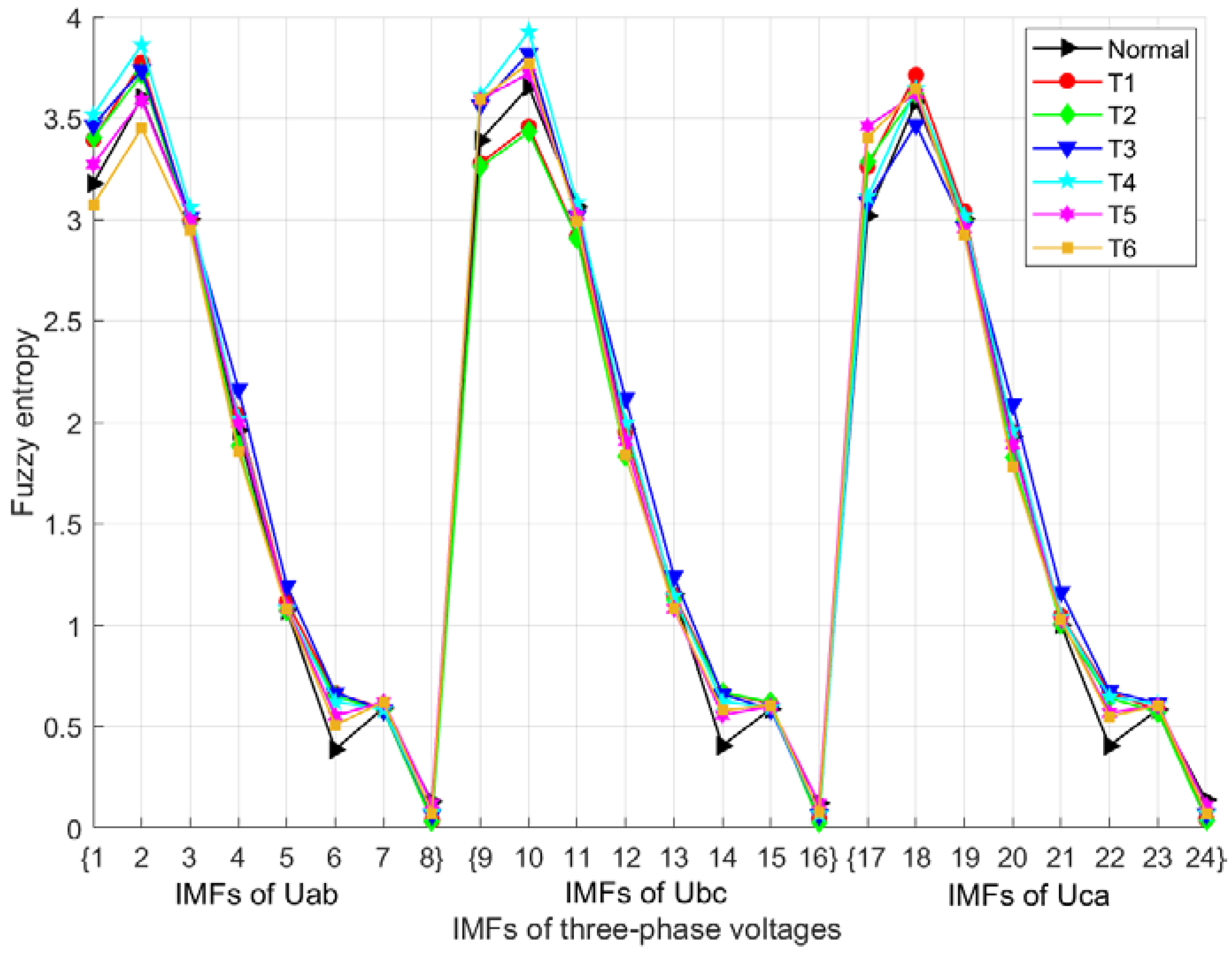
3.3. Feature Extraction Using FE

In order to visually represent the difference between different faults of the converter, it is necessary to extract distinctive fault feature information. Fuzzy entropy (FE) is a nonlinear dynamic index to measure the complexity of the system [35]; it can measure the irregularity of the system. Therefore, the FE of the system signal changes with the fault state of the system. Thus, the FE of IMF is calculated to form the fault feature vector. For a given signal $u(n)=\{u(1),u(2),\dots ,u(N)\}$, the FE is calculated as follows.

Step 1. Define embedding dimension $m(m\le N-2)$ and similarity tolerance $r$, then reconstruct the phase space:

$$\begin{array}{l}X(i) = \{u(i),u(i+1),\dots ,u(i+m-1)\}-u_0(i)\\ i=1, 2 , \dots , N-m+1\\ u_0(i)=\frac{1}{m}{\displaystyle \sum _{j=0}^{m-1}u(i+j)}\end{array}$$

(1)

Step 2. Introduce fuzzy membership function $A(x)$ to define the similarity of the vector space:

$$A(x)=\{\begin{array}{cc}1& x=0\\ \exp [-\ln 2{(x/r)}^{\alpha }]& x>0\end{array}$$

(2)

where $\alpha$ is weight, which determines the gradient of the similar tolerance boundary.

Calculate the similarity between $X(i)$ and $X(j)$:

$$\begin{array}{l}{A}_{ij}^m=\exp [-\ln 2{({\ell }_{ij}^m/r)}^{\alpha }]\\ j=1, 2 , \dots , N-m, and j\ne i\end{array}$$

(3)

where ${\ell }_{ij}^m$ is the maximum absolute difference between $X(i)$ and $X(j)$:

$$\begin{array}{l}{\ell }_{ij}^m=\ell [X(i),X(j) ]\\ =\underset{p=1,2,\dots ,m}{\max }(\left|u(i+p-1)-u_0(i)\right|-\left|u(j+p-1)-u_0(j)\right|)\end{array}$$

(4)

Step 3. Calculate the average value of $A_{ij}^m$:

$${\Psi }_i^m(\alpha ,r)=\frac{1}{N-m-1}{\displaystyle \sum _{j=1,j\ne i}^{N-m}{A}_{ij}^m}$$

(5)

Step 4. Define:

$${\Phi }^m(\alpha ,r)=\frac{1}{N-m}{\displaystyle \sum _{i=1}^{N-m}{\Psi }_i^m(r)}$$

(6)

Step 5. The fuzzy entropy of the signal is defined as:

$$FuzzyEn(m,\alpha ,r)=\ln {\Phi }^m(\alpha ,r)-\ln {\Phi }^{m+1}(\alpha ,r)$$

(7)

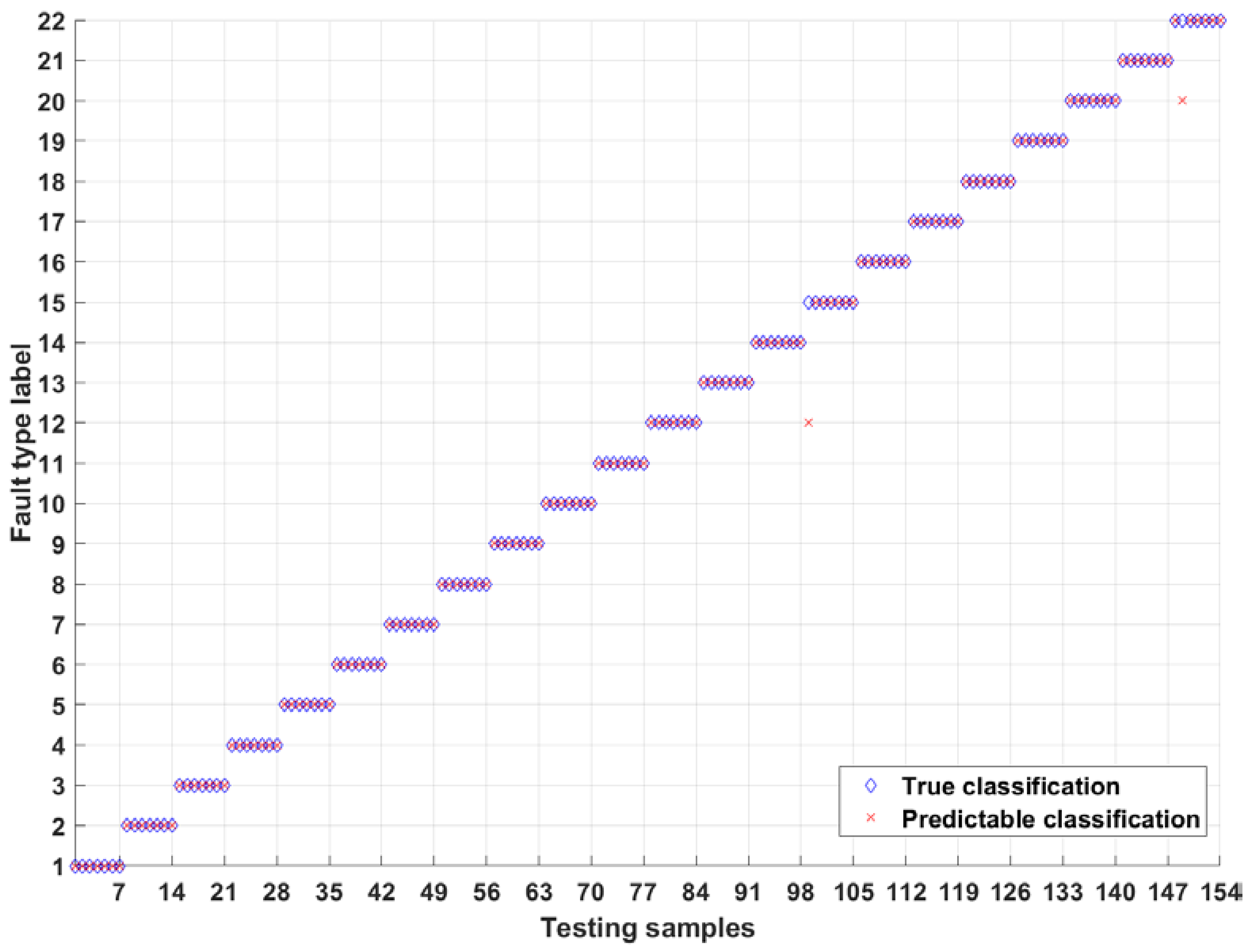
3.4. Fault Classification Diagnosis Using AFSA-SVM

SVM isolates different categories by establishing an optimal hyperplane [36]. For a dataset $G=\{(x_i,y_i),i=1,2,\dots ,I\}$, the classification decision function is defined as:

$$y_i=w^T\varphi (x_i)+\eta$$

(8)

where $x_i$ and  $y_i$ are the input sample and the corresponding category label, respectively. $\eta$ is offset, and $w$ is the weight vector orthogonal to the classification hyperplane.

Calculate the optimal hyperplane.

$$\underset{w,\eta ,\xi }{\min }\frac{1}{2}{w}^{T}w+C{\displaystyle \sum _{i=1}^I{\xi }_i}$$

(9)

subject to

$$\begin{array}{l}{y}_i(w^T\varphi (x_i)+\eta )\ge 1-{\xi }_i\\ {\xi }_i\ge 0,i=1,2,\dots ,I\end{array}$$

(10)

where $C$ is the penalty coefficient and ${\xi }_i$ is the slack variable.

$k(x_i,x_j)=\varphi {(x_i)}^T\varphi (x_j)$ is a kernel function. It is used to map linearly indivisible low-dimensional data to high-dimensional areas. The radial basis function is used in this paper:

$$k(x_i,x_j)=\exp (-\gamma {\Vert x_i-x_j\Vert }^2),\gamma >0$$

(11)

where $\gamma$ is the bandwidth of kernel function.

Penalty coefficient $C$ is used to adjust the ratio of confidence interval and empirical risk in the determined subspace to optimize the classification ability of the classifier. Kernel function parameter $\gamma$ reflects the distribution of data after mapping to feature space, and the suitable $\gamma$ can map the data to the proper feature space. $\gamma =\frac{1}{2{\sigma }^2}$, $\sigma$ is standard deviation.

The artificial fish swarm algorithm (AFSA) is a swarm intelligence optimization algorithm based on animal behavior [37]. The parameter optimization process of AFSA is realized by simulating the behavior of fish looking for food. AFSA has a simple structure, good global convergence, strong robustness, and fast speed. The penalty coefficient and kernel function parameter of SVM are optimized by AFSA, which avoids the problem of traditional methods falling into local optimization, improves the prediction accuracy of the model, and overcomes the problem of slow convergence of traditional methods. AFSA optimization steps are as follows:

Step 1. Initialization. Set population size $N$, individual state of artificial fish $X_i=\left\{x_1,x_2,\dots ,x_{\rho }\right\}$, food concentration $Y_i=f(X_i)$, distance between artificial fish ${\epsilon }_{ij}=\left|X_i-X_j\right|$, visual field of artificial fish $visual$, step length $step$, crowding factor $\zeta$, and number of foraging trials $\kappa$.

Step 2. The individuals in the fish school represent the parameters (C, σ) in the SVM model. Choose to use more cross-validation methods to seek the optimal parameters as the fitness function.

Step 3. Evaluate each individual and perform artificial fish behavior, including foraging, clustering, and rear-end.

Foraging behavior: Comparing the food concentration function $\mathsf{{\rm Y}}$ of the two times, the movement direction of the artificial fish is determined by the food concentration function $\mathsf{{\rm Y}}$. If ${\mathsf{{\rm Y}}}_i>{\mathsf{{\rm Y}}}_j$, move one step; otherwise, a state $X_j$ is selected at random for comparison. If the artificial fish cannot decide which way to move after several attempts, it moves one step at random. Suppose $rand(\cdot )$ represents any random number between 0 and 1, then a random state $X_j$ is represented as $X_j=X_i+rand(\cdot )\times visual$. The state of the artificial fish after moving one step is $X_{inext}$:

$$X_{inext}=\{\begin{array}{cc}{X}_i+rand(\cdot )\cdot step\cdot \frac{{{\displaystyle X}}_j - {{\displaystyle X}}_i}{\left|{{\displaystyle X}}_j - {{\displaystyle X}}_i\right|}& {{\displaystyle \mathsf{{\rm Y}}}}_i<{{\displaystyle \mathsf{{\rm Y}}}}_j\\ X_i+rand(\cdot )\cdot step& {{\displaystyle \mathsf{{\rm Y}}}}_i>{{\displaystyle \mathsf{{\rm Y}}}}_j\end{array}$$

(12)

Clustering behavior: Suppose the number of artificial fish in the current field of view is $\lambda$, the state of artificial fish in the cluster center is $X_{\mu }$. In the cluster center, the food concentration is ${\mathsf{{\rm Y}}}_{\mu }$. When $\frac{{\mathsf{{\rm Y}}}_{\mu }}{\lambda }>\delta {\mathsf{{\rm Y}}}_i$ indicates that the center is not crowded, the artificial fish moves toward the center; otherwise, foraging behavior is performed. The formula is as follows:

$$X_{inext}=\{\begin{array}{cc}{X}_i+rand(\cdot )\cdot step\cdot \frac{{{\displaystyle X}}_{\mu } - {{\displaystyle X}}_j}{\left|{{\displaystyle X}}_{\mu } - {{\displaystyle X}}_j\right|}& \frac{{\mathsf{{\rm Y}}}_{\mu }}{\lambda }>\delta {\mathsf{{\rm Y}}}_i\\ Foraging behavior& \frac{{\mathsf{{\rm Y}}}_{\mu }}{\lambda }<\delta {\mathsf{{\rm Y}}}_i\end{array}$$

(13)

Rear-end behavior: Suppose the position of artificial fish with high food concentration is denoted as $X_j$, corresponding to food concentration ${\mathsf{{\rm Y}}}_j$. If $\frac{{\mathsf{{\rm Y}}}_j}{\lambda }>\delta {\mathsf{{\rm Y}}}_i$ indicates that the food at state $X_j$ is more than the food at the current position and this position is not crowded, then the artificial fish moves one step to position $X_j$; otherwise, foraging behavior will be carried out, as follows:

$$X_{inext}=\{\begin{array}{cc}{X}_i+rand(\cdot )\cdot step\cdot \frac{{{\displaystyle X}}_j - {{\displaystyle X}}_i}{\left|{{\displaystyle X}}_j - {{\displaystyle X}}_i\right|}& \frac{{\mathsf{{\rm Y}}}_j}{\lambda }>\delta {\mathsf{{\rm Y}}}_i\\ Foraging behavior& \frac{{\mathsf{{\rm Y}}}_j}{\lambda }<\delta {\mathsf{{\rm Y}}}_i\end{array}$$

(14)

Step 4. After foraging, clustering and rear-end behavior, each individual replaces the better value by comparing the current state with the optimal value. Each individual reaches the optimal state after many iterations.

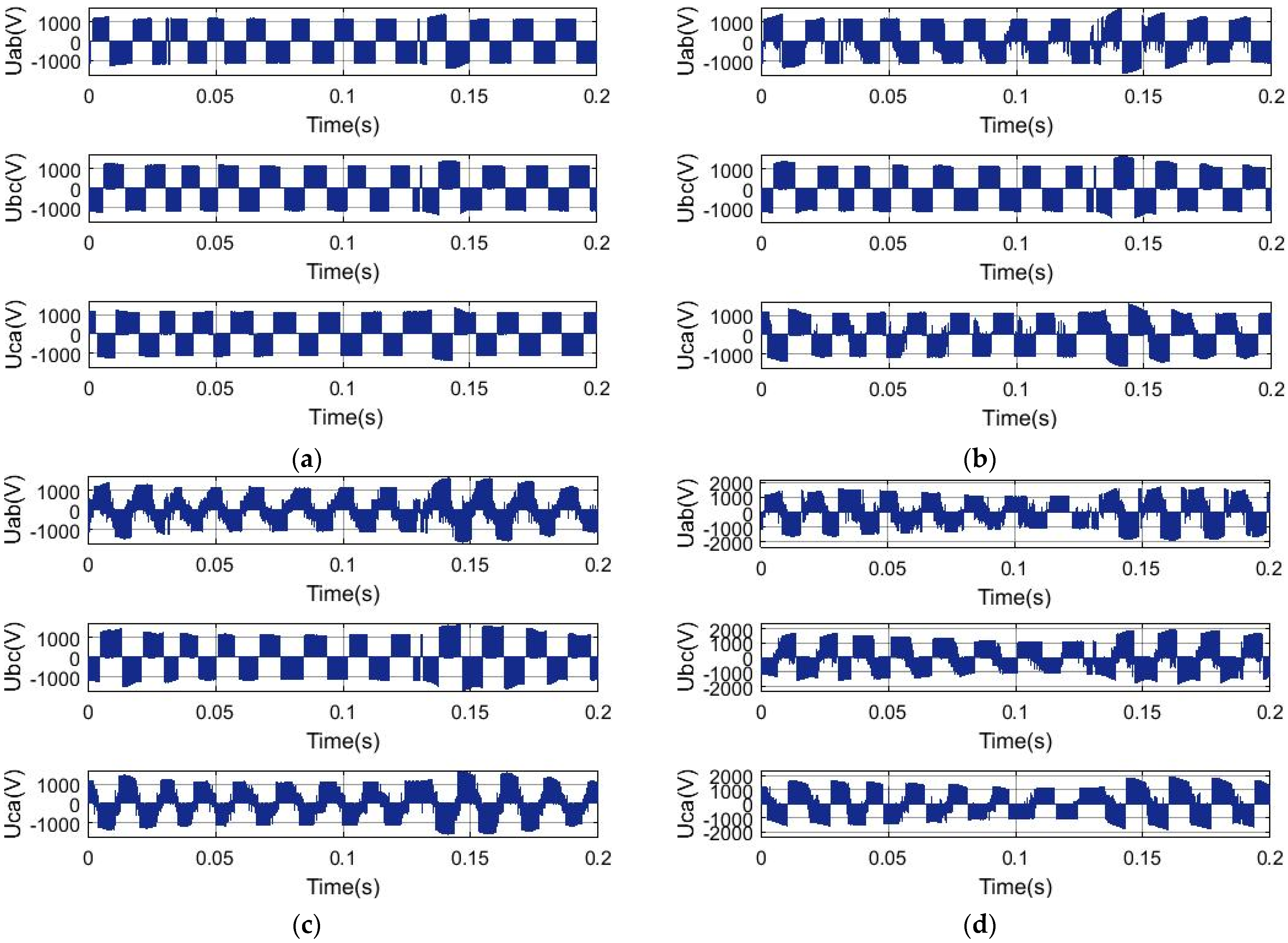
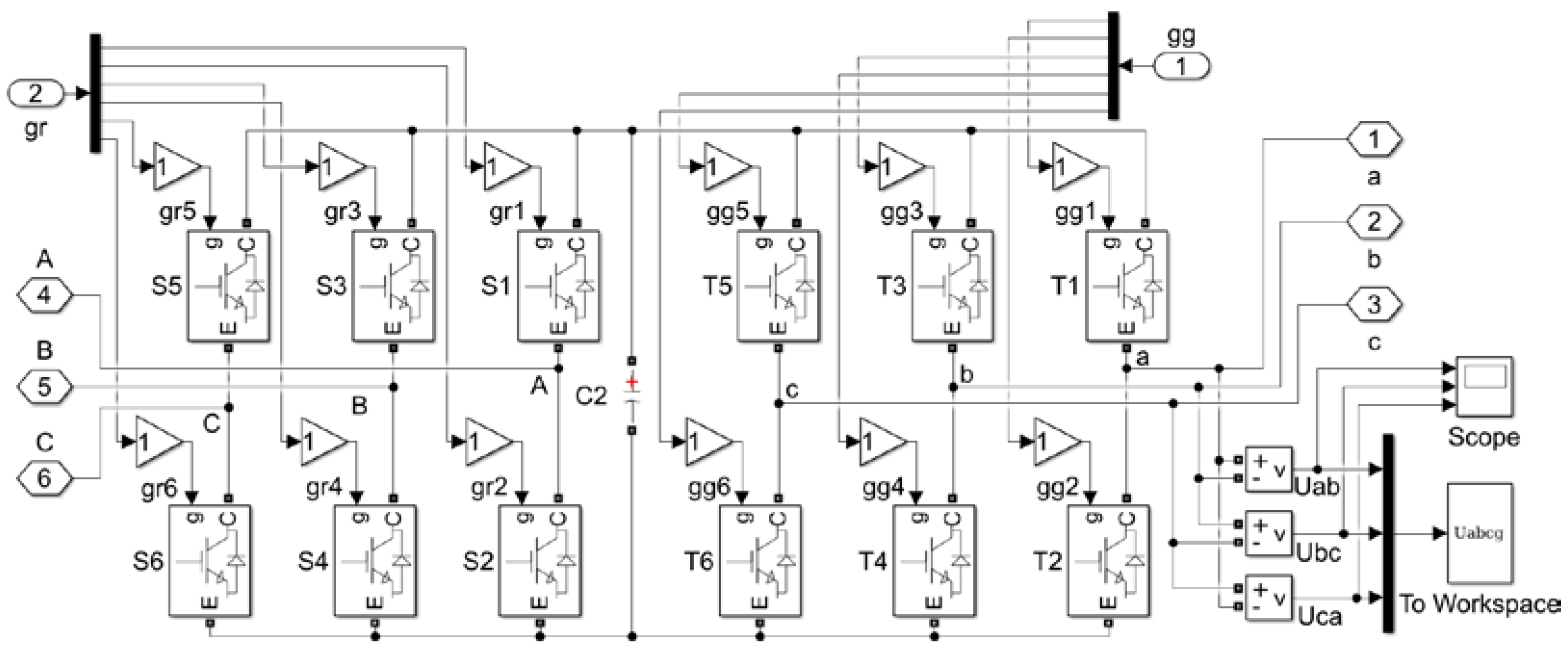
4. Simulation Results and Discussion

4.1. Simulation Platform

The DFIG wind power system simulation model is established to assess the performance of the proposed intelligent fault diagnosis method MEMD-FE-AFSA-SVM. The wind energy converter model is shown in Figure 3, and the main parameters are shown in

Table 2. Main parameters of the wind power system.

Quantity	Value	Quantity	Value
Nominal power	1.5 MW	Resistance of rotor	0.016 pu
Nominal voltage	575 V	Leak inductance of rotor	0.16 pu
Resistance of stator	0.023 pu	Pole pairs number	3
Leak inductance of stator	0.18 pu	Magnetizing inductance	2.9 pu

.

We set the sampling frequency of the simulation to 10 kHz and the sampling time to 1 s, and obtained the sample with the size of 10,000. The OC fault of IGBT is simulated by removing the corresponding gate signal; for instance, an OC fault is inserted in T1 by setting gg₁ to 0.

For assessing the robustness of the proposed fault diagnosis method to wind speed, the three-phase voltages U_ab, U_bc, and U_ca are measured when the wind speed varies from 10 m/s to 15 m/s, and the interval is 0.0625 m/s. Thus, there are 81 sets of three-channel signals as the original samples. For 22 fault modes, there are 1782 sets of original samples in total. In order to verify the robustness of the proposed fault diagnosis method to noise, white noise with different signal-to-noise ratios (30 dB, 20 dB, and 10 dB) is, respectively, added to the original voltage signals.

We perform MEMD decomposition on each set of three-channel samples, and the matching and aligned IMFs of each set of samples were obtained. Then, we calculated the fuzzy entropy of the IMFs as fault features of the converter, denoted as $[H_{FE}(\mathrm{IMFs}{/}_{U_{ab}}),H_{FE}(\mathrm{IMFs}{/}_{U_{bc}}),H_{FE}(\mathrm{IMFs}{/}_{U_{ca}})]$. Finally, we input the fault feature samples into the AFSA-SVM model to identify the fault modes. Randomly select the training samples and test samples under each fault state, and the number of training samples is larger than that of test samples.

4.2. Results of Decomposition

MEMD is used to extract the common mode of the three-phase voltages U_ab, U_bc, and U_ca matching with the aligned timescale. Figure 4a shows these scale-aligned modes in the order of timescales from small to large. In order to highlight the advantages of MEMD, the EMD decomposition results are shown in Figure 4b.

From Figure 4a, there are the same number of IMF components in each group of IMFs by MEMD, and U_ab, U_bc, and U_ca are all decomposed into 14 IMFs. Furthermore, the IMF in different voltages has the same frequency on the same timescale, such as the IMF8 (marked in red box), and the frequencies of U_ab, U_bc, and U_ca are essentially equal. Thus, MEMD solves the difficulty of matching and aligning the number and frequency of IMFs in U_ab, U_bc, and U_ca.

As shown in Figure 4b, the number of IMFs obtained from each signal decomposition is different; U_ab is decomposed into 15 IMF components by EMD, while U_bc and U_ca are decomposed into 14 IMFs and 13 IMFs, respectively. In addition, IMF frequencies of different signals in the same order are different; for example, for IMF10 (marked in the green box), the frequency of U_ab is the largest, followed by the frequency of U_bc, and the frequency of U_ca is the smallest. As a result, the IMF sets of the three-phase voltage signals U_ab, U_bc, and U_ca by EMD decomposition do not match in quantity and frequency. This is because the EMD decomposition process of U_ab, U_bc, and U_ca is independent for each signal without considering the internal correlation.

In order to more accurately verify the superiority of the results, the corresponding timescales measured by FFT are shown in

Table 3. The timescales of the common modes extracted by MEMD.

Mode	Uab	Ubc	Uca
IMFs 1	2.14	2.14	2.14
IMFs 2	3.87	3.87	3.87
IMFs 3	9.08	6.02	9.08
IMFs 4	11.61	13.49	11.61
IMFs 5	19.96	19.96	19.96
IMFs 6	54.95	38.31	38.31
IMFs 7	82.65	82.65	82.65
IMFs 8	277.80	277.80	277.80
IMFs 9	526.36	588.29	588.29
IMFs 10	909.18	909.18	909.18
IMFs 11	2000.20	2000.20	2000.20
IMFs 12	3333.66	3333.66	3333.66
IMFs 13	5000.50	5000.50	5000.50
res	5000.50	>T	5000.50

Note: T = 10,000 is the length of the sample.

and

Table 4. The timescales of the common modes extracted by EMD.

Mode	Uab	Ubc	Uca
IMFs 1	2.14	2.14	2.14
IMFs 2	5.61	4.67	6.02
IMFs 3	9.08	6.02	9.08
IMFs 4	13.49	13.49	13.49
IMFs 5	19.96	19.96	19.96
IMFs 6	19.96	49.75	41.49
IMFs 7	82.65	82.65	163.95
IMFs 8	163.95	322.61	344.86
IMFs 9	312.53	500.05	625.06
IMFs 10	500.05	833.41	1666.83
IMFs 11	1111.22	2000.20	2500.25
IMFs 12	2000.20	2500.25	3333.66
IMFs 13	3333.66	3333.66	>T
IMFs 14	3333.66	>T	-
res	>T	-	-

Note: T = 10,000 is the length of the sample.

.

As shown in Table 3, MEMD effectively captures the common characteristics of three-phase voltage signals, and its timescale is basically the same within the same group, but different between groups. In particular, the timescales of IMFs 7–8 and IMFs 10–13 have no difference within the group and no overlap between groups. Although there is intra-group difference in IMFs 9, it is very small, which is far less than the difference between groups with IMFs 8 and IMFs 10. Therefore, such a satisfactory analysis is helpful for the subsequent feature extraction, thus improving the accuracy of converter fault diagnosis.

The results in Table 4 show that although the intra-group differences in IMFs 1–4 are relatively small, there is inter-group overlap of U_ab between IMF 5 and IMF 6. In addition, the timescale misalignment occurs from IMFs 6. For example, the timescales of IMF 10 are 500.05, 833.41, and 1666.83, and the intra-group difference completely exceeds the inter-group difference. Therefore, compared with MEMD, the analysis results of EMD are very unsatisfactory, and serious mode mixing occurs.

Because MEMD directly acts on three-phase voltage signals U_ab, U_bc, and U_ca at the same time, it provides internal information about the interaction of the three voltages, providing physical insight into the operation status of the converter system. Therefore, the signal processing of MEMD reduces the difficulty of subsequent fault diagnosis.

The adaptive decomposition characteristic of MEMD results in the outcome that the number of IMFs obtained after the decomposition of 1782 sets of data samples in 22 fault modes may not be equal. After decomposition, the minimum number of IMFs of all samples is calculated to be eight.

4.3. Results of Feature Extraction

The calculation of fuzzy entropy mainly involves three parameters: $m$, $r$, and $\alpha$. A larger $m$ can reconstruct the dynamic process of the system in more detail. However, the larger the $m$, the longer data length required. Generally, the data length is ${10}^m~{30}^m$. According to the length of converter simulation data 10,000, $m$ is chosen as 3. $r$ determines the width of the boundary of the fuzzy function. Too large an $r$ causes information loss, while too small an $r$ will increase the sensitivity of the result to noise. When $r=0.2std$, where $std$ is the signal standard deviation, not only is the complete feature information retained, but also the robustness is guaranteed. $\alpha$ represents the boundary gradient, and too large an $\alpha$ will cause information loss; the value of 2 can increase the probability of similarity between the nearest vectors’ weights. The fuzzy entropy results of the MEMD-IMFs of three-phase voltages in different fault modes are shown in Figure 5.

Figure 5 shows that there are significant differences between fuzzy entropy values under different converter fault states, especially IMF1 and IMF2 for U_ab, IMF10 for U_bc, and IMF17 for U_ca. Thus, fuzzy entropy can measure the complexity of the three-phase voltages. Therefore, it is reasonable to use fuzzy entropy as a feature vector to characterize and observe different fault modes of the converter.

4.4. Results of Classification

We added 30 dB white noise to the original voltage signals, and input the extracted IMF-FE fault features into the AFSA-SVM classifier for training and testing to realize intelligent fault diagnosis. We set the relevant parameters of the AFSA algorithm as follows: population size is 20, number of iterations is 50, congestion factor is 0.3, visual is 10, step length is 1.25, and number of foraging trials is 5. The diagnostic results of the AFSA-SVM classification model are shown in Figure 6.

As shown in Figure 6, among 154 testing samples with 22 fault modes, only 2 samples are identified incorrectly, and the rest are all correctly output; thus, the diagnostic accuracy of the AFSA-SVM model is 98.7%. The results show that the proposed fault diagnosis method can diagnose the converter fault accurately and effectively. Therefore, this method has strong robustness to wind speed and noise in a wind power generation system.

4.5. Comparison of Different Methods

In order to evaluate the reliability and robustness of the proposed fault diagnosis method MEMD-FE-AFSA-SVM for converters, different feature extraction methods combined with the AFSA-SVM classification model for all the noise conditions (30 dB, 20 dB, and 10 dB) are compared, including MEMD-FE, EMD-FE, and MEMD-sample entropy (SE). The simulations were run 30 times and we recorded the maximum, minimum, and average value of accuracy, as well as standard deviations. The results are shown in

Table 5. Comparison of diagnosis results with different feature extraction methods.

Noise Level	Different Methods	Accuracy (%)
		Maximum	Minimum	Average	Standard Deviation
30 dB	MEMD-FE	99.7532	91.3117	95.5758	1.9344
	EMD-FE	84.1688	79.6234	82.0260	3.4044
	MEMD-SE	99.1039	91.9610	95.2727	2.3996
20 dB	MEMD-FE	93.6250	89.6477	92.1477	1.3312
	EMD-FE	76.3766	60.1429	69.8182	4.6368
	MEMD-SE	92.5065	86.7662	90.4286	2.8846
10 dB	MEMD-FE	86.1169	82.2727	84.2338	1.7167
	EMD-FE	65.9870	58.1948	63.0000	3.1679
	MEMD-SE	80.4148	73.3125	76.3807	2.5971

.

As shown in Table 5, the average diagnostic accuracies of the MEMD-FE method at all noise levels are higher than 84%, and the standard deviations are lower than 2%, indicating that this method has good noise robustness and stability. Although the average accuracy of the MEMD-SE method is close to that of the MEMD-FE method at 30 dB and 20 dB, the standard deviation of the MEMD-SE method is very large, about 2.4% at 30 dB and 2.9% at 20 dB, so the stability of the MEMD-SE method is not as good as that of the MEMD-FE method. Moreover, the average diagnostic accuracy of the MEMD-FE method at 10 dB (84.2338%) is significantly higher than that of the MEMD-SE method at 10 dB (76.3807%), thus, the noise robustness of the MEMD-FE method is better than that of the MEMD-SE method. It can be seen from Table 5 that the average accuracy of the EMD-FE method is significantly lower than that of the MEMD-FE method at all noise levels, and its standard deviation is greater than 3% at all noise levels. As a result, the MEMD-FE method has stronger noise robustness and higher stability than the EMD-FE method.

To sum up, the MEMD-FE method is optimal; it is strong and robust enough to withstand noise, and it is very stable and reliable.

In order to verify the advantages of AFSA, different methods based on MEMD-FE features combined with different optimized SVM algorithms are compared, including AFSA-SVM, CS-SVM, PSO-SVM, GA-SVM, and CV-SVM. Running 30 times, the accuracy and computing time of different optimization SVM classification models for all the noise conditions (30 dB, 20 dB, and 10 dB) were recorded as shown in

Table 6. Comparison of diagnosis results with different classification models.

Noise Level	Different Methods	Accuracy (%)				Time (s)
		Maximum	Minimum	Average	Standard Deviation	Maximum	Minimum	Average	Standard Deviation
30 dB	AFSA-SVM	99.7532	91.3117	95.5758	1.9344	515.9140	437.5331	484.7235	19.5119
	CS-SVM	93.2597	77.6753	85.4675	7.3005	1.2609 × 10³	439.8244	811.4330	337.8004
	GA-SVM	95.1875	86.5227	91.9631	2.4902	1.2842 × 10³	1.0122 × 10³	1.1841 × 10³	91.7936
	PSO-SVM	94.1558	81.1688	90.3896	5.2833	2.1020 × 10³	1.9771 × 10³	2.0466 × 10³	44.6337
	CV-SVM	95.0519	88.9610	92.0130	2.8886	224.5880	214.4492	223.4154	3.1523
20 dB	AFSA-SVM	93.6250	89.6477	92.1477	1.3312	573.9010	496.1134	536.6309	25.9141
	CS-SVM	88.6104	69.4805	82.3896	7.9602	924.5070	597.9579	736.4997	168.8008
	GA-SVM	90.8571	83.0130	87.0433	2.9281	1.1761 × 10³	1.1144 × 10³	1.1422 × 10³	31.2674
	PSO-SVM	89.4545	79.0649	86.9091	5.3152	2.7518 × 10³	2.6897 × 10³	2.7298 × 10³	34.8368
	CV-SVM	90.5864	82.4156	88.8571	3.0546	420.1174	410.2499	416.5160	2.8462
10 dB	AFSA-SVM	86.1169	82.2727	84.2338	1.7167	821.9604	727.2384	771.6015	29.3344
	CS-SVM	82.7143	65.3247	76.7370	7.2453	2.0202 × 10³	1.1984 × 10³	1.5256 × 10³	299.4243
	GA-SVM	82.7662	76.2208	80.3853	2.5804	1.8279 × 10³	1.6829 × 10³	1.7595 × 10³	72.8349
	PSO-SVM	83.4156	72.0779	79.7078	5.7196	3.7101 × 10³	3.6438 × 10³	3.6783 × 10³	30.0669
	CV-SVM	83.1169	72.0779	78.0519	3.5672	313.5173	311.3903	311.8531	0.6606

, including the maximum, minimum, average, and standard deviation.

Table 6 shows that the average accuracy of the AFSA-SVM classification model is significantly higher than other classification models in all noise levels, and its standard deviation is the smallest. Although the average accuracy of the GA-SVM method, PSO-SVM method, and CV-SVM method is higher than 90% at 30 dB, their standard deviation is large, exceeding 2.4%, and the standard deviation of the PSO-SVM method even exceeds 5.2%. Therefore, compared with other optimized classification models, the AFSA-SVM method not only has good noise robustness, but also has stable diagnostic performance. In addition, the average computing time of the AFSA-SVM method (484.7235 s) is significantly lower than that of CS-SVM (811.4330 s), GA-SVM (1.1841 × 10³ s) and PSO-SVM (2.0466 × 10³ s) at 30 dB, thus, the AFSA optimization algorithm has the advantage of high computing efficiency compared with other methods. Furthermore, the standard deviation of calculation time of AFSA-SVM is the smallest (19.5119 s), and that of CS-SVM is very large, over 337 s, so the optimization calculation of the AFSA method is more stable. Although the average value and standard deviation of the calculation time of the CV-SVM method surpass that of the AFSA-SVM method, its diagnostic accuracy is significantly lower than that of the AFSA-SVM method. Therefore, the AFSA-SVM classification model has outstanding advantages in accuracy and computational efficiency.

To sum up, the fault diagnosis method MEMD-FE-AFSA-SVM proposed in this paper not only has high diagnosis accuracy and strong robustness, but also high computational efficiency. Therefore, it has practical application value.

5. Conclusions

In order to increase the durability of wind energy converters, this paper presents a new hybrid fault diagnosis method for wind energy converters based on multivariate empirical mode decomposition (MEMD), fuzzy entropy (FE), and an artificial fish swarm algorithm (AFSA)-support vector machine (SVM). Three-phase voltage signals of the converter are directly and simultaneously decomposed by MEMD, realizing the matching and alignment of the number and frequency of IMFs in the multi-channel signals. MEMD provides internal information about the interaction of the three-phase voltage signals, achieving physical insight into the converter operating states. The results show that the method has strong robustness to wind speed variation, and the final diagnostic accuracy of 22 fault modes is 98.7% for different wind speeds. The FE reflecting the complexity of intrinsic oscillations is used to construct fault feature vectors and input into AFSA-optimized SVM; this increases the robustness to noise, and the average accuracy can reach 95.5758% at 30 dB noise. The superiority of this method is verified by strict comparison of different methods.

As an effective fault diagnosis tool, the method proposed in this paper can be extended to fault diagnosis based on multi-source signals. This method can also be applied to other converter systems. This study only considers the impact of wind speed and noise in the wind power system, and it will be fascinating to study the applicability of more variable operating conditions. In future work, it also will be interesting to explore new robust feature extraction methods and more time-efficient model optimization algorithms for actual engineering applications.

References

1. Papadopoulos, P.; Coit, D.W.; Ezzat, A.A. Seizing Opportunity: Maintenance Optimization in Offshore Wind Farms Considering Accessibility, Production, and Crew Dispatch. IEEE Trans. Sustain. Energy 2022, 13, 111. [Google Scholar] [CrossRef]
2. Saidi, L.; Benbouzid, M. Prognostics and Health Management of Renewable Energy Systems: State of the Art Review, Challenges, and Trends. Electronics 2021, 10, 2732. [Google Scholar] [CrossRef]
3. Guo, Y.; Sheng, S.; Phillips, C.; Keller, J.; Veers, P.; Williams, L. A methodology for reliability assessment and prognosis of bearing axial cracking in wind turbine gearboxes. Renew. Sustain. Energy Rev. 2020, 127, 109888. [Google Scholar] [CrossRef]
4. Nie, X.; Liu, S.; Xie, G. A Novel Autoencoder with Dynamic Feature Enhanced Factor for Fault Diagnosis of Wind Turbine. Electronics 2020, 9, 600. [Google Scholar] [CrossRef] [Green Version]
5. Li, S.; Cao, B.; Li, J.; Cui, Y.; Kang, Y.; Wu, G. Review of condition monitoring and defect inspection methods for composited cable terminals. High Volt. 2023. [Google Scholar] [CrossRef]
6. Artigao, E.; Martínez, S.; Escribano, A.; Lázaro, E. Wind turbine reliability: A comprehensive review towards effective condition monitoring development. Appl. Energy 2018, 228, 1569. [Google Scholar] [CrossRef]
7. Liang, J.; Zhang, K.; Durra, A.A.; Muyeen, S.M.; Zhou, D. A state-of-the-art review on wind power converter fault diagnosis. Energy Rep. 2022, 8, 5341. [Google Scholar] [CrossRef]
8. Guang, X.; Wang, Z.; Li, L.; Su, Q. Robust fault diagnosis for closed-loop grid-connected inverter based on sliding mode observer and identifier. Electr. Power Syst. Res. 2023, 217, 109097. [Google Scholar]
9. Jia, H.; Deng, Y.; Hu, X.; Deng, Z.; He, X. A Concurrent Diagnosis Method of IGBT Open-Circuit Faults in Modular Multilevel Converters. IEEE J. Emerg. Sel. Top. Power Electron. 2023. [Google Scholar] [CrossRef]
10. Zhao, H.; Cheng, L. Open-circuit faults diagnosis in back-to-back converters of DF wind turbine. IET Renew. Power Gener. 2017, 11, 417. [Google Scholar] [CrossRef]
11. Qiu, Y.; Jiang, H.; Feng, Y.; Cao, M.; Zhao, Y.; Li, D. A new fault diagnosis algorithm for PMSG wind turbine power converters under variable wind speed conditions. Energies 2016, 9, 548. [Google Scholar] [CrossRef]
12. Wang, T.; Xu, H.; Han, J.; Elbouchikhi, E.; Benbouzid, M.E. Cascaded H-bridge multilevel inverter system fault diagnosis using a PCA and multiclass relevance vector machine approach. IEEE Trans. Power Electron. 2015, 30, 7006. [Google Scholar] [CrossRef]
13. Wang, T.; Qi, J.; Xu, H.; Wang, Y.; Liu, L.; Gao, D. Fault diagnosis method based on FFT-RPCA-SVM for cascaded-multilevel inverter. ISA Trans. 2016, 60, 156. [Google Scholar] [CrossRef] [PubMed]
14. Cai, B.; Zhao, Y.; Liu, H.; Xie, M. A data-driven fault diagnosis methodology in three-phase inverters for PMSM drive systems. IEEE Trans. Power Electron. 2017, 32, 5590. [Google Scholar] [CrossRef]
15. Wu, F.; Hao, Y.; Zhao, J.; Liu, Y. Current similarity based open-circuit fault diagnosis for induction motor drives with discrete wavelet transform. Microelectron. Reliab. 2017, 75, 309. [Google Scholar] [CrossRef]
16. Dhumale, R.B.; Lokhande, S.D. Neural network fault diagnosis of voltage source inverter under variable load conditions at different frequencies. Measurement 2016, 91, 565. [Google Scholar] [CrossRef]
17. Liu, Y.; Chai, Y.; Wei, S.; Luo, Z. Circuit Fault diagnostic method of Wind Power Converter with Wavelet-DBN. Chin. Intell. Syst. Conf. CISC 2017, 460, 623. [Google Scholar]
18. Huang, N.E.; Shen, Z.; Long, S.R.; Wu, M.C.; Shih, H.H.; Zheng, Q.; Yen, N.-C.; Tung, C.C.; Liu, H.H. The empirical mode decomposition and the Hilbert spectrum for nonlinear and non-stationary time series analysis. Proc. R. Soc. London. Ser. A Math. Phys. Eng. Sci. 1998, 454, 903–995. [Google Scholar] [CrossRef]
19. Beibei, M.; Shen, Y.; Wu, D.; Zhao, Z. Three level inverter fault diagnosis using EMD and support vector machine approach. In Proceedings of the 12th IEEE Conference on Industrial Electronics and Applications (ICIEA), Siem Reap, Cambodia, 18–20 June 2017. [Google Scholar]
20. Liang, J.; Zhang, K.; Durra, A.A.; Zhou, D. A novel fault diagnostic method in power converters for wind power generation system. Appl. Energy 2020, 266, 114851. [Google Scholar] [CrossRef]
21. Cherif, B.; Bendiabdellah, A.; Tabbakh, M. An Automatic Diagnosis of an Inverter IGBT Open-Circuit Fault Based on HHT-ANN. Electr. Power Compon. Syst. 2020, 48, 589. [Google Scholar] [CrossRef]
22. Yan, X.; Liu, Y.; Xu, Y.; Jia, M. Multichannel fault diagnosis of wind turbine driving system using multivariate singular spectrum decomposition and improved Kolmogorov complexity. Renew. Energy 2021, 170, 724–748. [Google Scholar] [CrossRef]
23. Yang, Y.; Zhu, W. Research Based on Improved CNN-SVM Fault Diagnosis of V2G Charging Pile. Electronics 2023, 12, 655. [Google Scholar] [CrossRef]
24. Liu, Z.; Li, M.; Zhu, Z.; Xiao, L.; Nie, C.; Tang, Z. Health State Identification Method of Nuclear Power Main Circulating Pump Based on EEMD and OQGA-SVM. Electronics 2023, 12, 410. [Google Scholar] [CrossRef]
25. Ke, L.; Liu, Z.; Zhang, Y. Fault Diagnosis of Modular Multilevel Converter Based on Optimized Support Vector Machine. In Proceedings of the 2020 39th Chinese Control Conference (CCC), Shenyang, China, 27–30 July 2020; pp. 4204–4209. [Google Scholar]
26. Cai, X.; Wai, R.J. Intelligent DC Arc-Fault Detection of Solar PV Power Generation System via Optimized VMD-Based Signal Processing and PSO–SVM Classifier. IEEE J. Photovolt. 2022, 12, 1058. [Google Scholar] [CrossRef]
27. Shakya, S. Performance Analysis of Wind Turbine Monitoring Mechanism Using Integrated Classification and Optimization Techniques. J. Artif. Intell. Capsul. Netw. 2020, 2, 31. [Google Scholar] [CrossRef]
28. Chen, W.; Bazzi, A. Logic-based methods for intelligent fault diagnosis and recovery in power electronics. IEEE Trans. Power Electron. 2017, 32, 5573. [Google Scholar] [CrossRef]
29. Tan, Y.; Zhang, H.; Zhou, Y. Fault Detection Method for Permanent Magnet Synchronous Generator Wind Energy Converters Using Correlation Features Among Three-phase Currents. J. Mod. Power Syst. Clean Energy 2020, 8, 168. [Google Scholar] [CrossRef]
30. Gao, Y.; Wang, L.; Zhang, Y.; Yin, Z. Research on AC Arc Fault Characteristics Based on the Difference between Adjacent Current Cycle. In Proceedings of the Prognostics and System Health Management Conference (PHM-Qingdao), Qingdao, China, 25–27 October 2019. [Google Scholar]
31. Yuan, Y.; Chai, Y.; Qu, J.; Yang, Z.; Xu, S. Circuit fault diagnostic method of wind power converter with VMD-SVM. In Proceedings of the 35th Chinese Control Conference (CCC), Chengdu, China, 27–29 July 2016. [Google Scholar]
32. Baghli, M.; Delpha, C.; Diallo, D.; Hallouche, A.; Mba, D.; Wang, T. Three-level NPC inverter incipient fault detection and classification using output current statistical analysis. Energies 2019, 12, 1372. [Google Scholar] [CrossRef] [Green Version]
33. Rehman, N.; Mandic, D.P. Multivariate empirical mode decomposition. Proc. R. Soc. A 2010, 466, 1291. [Google Scholar] [CrossRef]
34. Rilling, G.; Flandrin, P.; Goncalves, P. On empirical mode decomposition and its algorithms. IEEE-EURASIP Workshop Nonlinear Signal Image Process. 2003, 3, 8–11. [Google Scholar]
35. Chen, W.; Wang, Z.; Xie, H.; Yu, W. Characterization of surface EMG signal based on fuzzy entropy. IEEE Trans. Neural. Syst. Rehabil. Eng. 2007, 15, 266. [Google Scholar] [CrossRef] [PubMed]
36. Vapnik, V.N. The Nature of Statistical Learning Theory; Springer: New York, NY, USA, 1995. [Google Scholar]
37. Liu, W.; Shen, J.; Yang, X. Rolling bearing fault detection approach based on improved dispersion entropy and AFSA optimized SVM. Int. J. Electr. Eng. Educ. 2020, 15, 1. [Google Scholar] [CrossRef]
Figure 1. The topology of a wind turbine system.
Electronics 12 01263 g001
Figure 2. The simulated voltage Uabcg (Uab, Ubc, Uca). (a) Normal state; (b) OC fault occurred in T1; (c) OC fault occurred in T1 and T2; (d) OC fault occurred in T1 and T3.
Electronics 12 01263 g002
Figure 3. Simulation model of the converter.
Electronics 12 01263 g003
Figure 4. The decomposition results of the three-phase voltages Uab, Ubc, and Uca. (a) MEMD; (b) EMD.
Electronics 12 01263 g004aElectronics 12 01263 g004b
Figure 5. The fuzzy entropy of the MEMD-IMFs of three-phase voltages in different fault modes.
Electronics 12 01263 g005
Figure 6. Diagnostic results of AFSA-SVM model.
Electronics 12 01263 g006