Siamese PointNet: 3D Head Pose Estimation with Local Feature Descriptor

Abstract

Head pose estimation is an important part of the field of face analysis technology. It can be applied to driver attention monitoring, passenger monitoring, effective information screening, etc. However, illumination changes and partial occlusion interfere with the task, and due to the non-stationary characteristic of the head pose change process, normal regression networks are unable to achieve very accurate results on large-scale synthetic training data. To address the above problems, a Siamese network based on 3D point clouds was proposed, which adopts a share weight network with similar pose samples to constrain the regression process of the pose’s angles; meanwhile, a local feature descriptor was introduced to describe the local geometric features of the objects. In order to verify the performance of our method, we conducted experiments on two public datasets: the Biwi Kinect Head Pose dataset and Pandora. The results show that compared with the latest methods, our standard deviation was reduced by 0.4, and the mean error was reduced by 0.1; meanwhile, our network also maintained a good real-time performance.

1. Introduction

Head pose estimation is an important part of the field of computer vision and also an important indicator for studying human behavior and attention. It can provide key information for many facial analysis tasks, such as face recognition, facial expression recognition, and driving concentration prediction [1]. The essence of the task is to predict the three pose angles (roll pitch yaw) of the object relative to the sensors. An effective algorithm should include the following main factors: a high accuracy, real-time performance, and the ability to cope with partial occlusion and large pose variations [2]. With respect to the above factors, many RGB-based head pose estimation algorithms have been proposed and achieved a very good performance [2]. However, the imaging quality of ordinary RGB sensors depends on light conditions, making them difficult to apply in some scenarios where light is weak or variable, such as night driving concentration detection, expression recognition in weak light environments, etc. [3]. With the development of depth sensors, it is more convenient to obtain high-quality depth images (also known as 2.5D images) [4]. Compared with ordinary RGB sensors, depth cameras have the following two main advantages. One advantage is that their infrared-based imaging principle—where each pixel represents the distance from the target to the sensors—makes the imaging quality mainly related to distances and is stable against variations in the light conditions; thus, it can be safely applied to human daily life [3]. The other advantage is that it can easily achieve background separation based on distance information, which can reduce the interference of the background and enable the task to focus on the object itself [1]. Depth maps can be easily converted into 3D point clouds by a simple coordinate transformation, which enables point clouds to inherit the above advantages of depth maps. Meanwhile, point clouds can better describe the spatial geometric feature of objects in 3D space, and the contours are stretched to have a more hierarchical appearance and clearer outlines; some important information around the outlines can be well retained [5].

Recently, many 3D methods based on different data types were proposed for face analysis, such as mesh, voxel grid, octree, and surface normal map. Compared with these four data types, the mathematical expression of a point cloud is more concise and can directly represent the spatial geometry information of an object. However, the disorder of the point clouds makes them difficult to apply to deep learning. Pioneers Qi et al. [6] relied on the idea of symmetric functions to solve the disorder of 3D point clouds and constructed PointNet. Many point clouds deep learning networks were proposed, such as those by Qi et al. [7], who optimized PointNet and proposed PointNet++. Deng et al. [8] introduced a local region representation to extract local features. Many point cloud methods were proposed for 3D computer vision. However, in the field of head pose estimation, due to the lack of the detailed textures of point clouds, the current pose estimation methods have not focused much attention on the local features of original point clouds, which leads to larger errors under large pose variations. Meanwhile, due to the non-stationary characteristic of the pose change process, previous regression networks were unable to achieve very good results on large-scale synthetic training data [9]. In order to deal with the above problems, we introduce a local feature descriptor coupled with a Siamese regression network for 3D head pose estimation. In our method, we first employ a local feature descriptor to describe the spatial geometric features of the objects; then, a group of PointNets is adopted to extract the local features, and three fully connected layers are used to map the head features to pose angles. Second, we utilize a share weight regression network with similar pose samples to guide the regression process of the pose angles. Finally, a novel loss function is introduced to constrain the difference between two similar features. In order to verify the effectiveness of the proposed method, we conduct experiments on two public datasets: the Biwi Kinect Head Pose dataset and Pandora.

The main contributions of this paper are summarized as follows:

• We introduce a local feature descriptor to describe the detailed features of the point clouds to reduce the impact of their lack of detailed texture.
• We present a new Siamese network to constrain the regression process of 3D head pose angles, which significantly reduced the errors of the original regression network. To the best of our knowledge, this is the first work to estimate 3D head poses by using a Siamese network.
• The experimental results on public datasets show that our accuracy outperforms the latest approaches and also exhibits a good real-time performance.

2. Related Works

In recent years, the most widely used head pose estimation methods have mainly been proposed on RGB images. Drouard et al. [10] extracted HOG-based descriptors from face bounding boxes and mapped them to the corresponding head poses. Patacchiola et al. [11] proposed a convolutional neural network (CNN) supplemented with adaptive gradient methods to make the method robust for real-world applications. Hsu et al. [9] adopted a classification network to supervise the regression process of pose angles, which significantly improved the accuracy of the head pose estimation. Ruiz et al. [12] jointly combined pose classification and regression training with a multi-loss convolutional neural network on a large synthetically expanded dataset, which reduced the dependence on landmarks and enhanced the robustness of the network. Recently, Huang et al. [13] introduced a head pose estimation method using two-stage ensembles with average top-k regression, which combined the two subtasks by considering the task-dependent weights instead of setting coefficients by using grid search. Based on the driver’s head pose and multi-head attention, Mercat et al. [14] proposed a vehicle motion forecasting method. In order to cope with complex situations, Liu et al. [15] proposed a robust three-branch model with a triplet module and matrix Fisher distribution module. Considering the discontinuity of Euler angles or quaternions and the observation that MAE may not reflect the actual behavior, Cao et al. [16] proposed an annotation method which uses three vectors to describe the head poses and measurements using the mean absolute error of the vectors (MAEV) to assess the performance. Relying on head poses, Jha et al. [17] proposed a formulation based on probabilistic models to create salient regions describing the driver’s visual attention. In order to bridge the gap between better predictions and incorrectly labeled pose images, Liu et al. [18] introduced probability values to encode labels, which took advantage of the adjacent pose’s information and achieved a very good performance.

Compared to RGB images, depth maps cope well with dramatic light changes but lack texture detail [5], and very few studies only rely on depth maps [3]. Ballotta et al. [4] constructed a fully convolutional network to predict the location of the head’s center. Wang et al. [19] combined the perception of deep learning and the decision-making power of machine learning to propose a convolutional neural network for multi-target head center localization. Borghi et al. [1] converted the depth maps into gray-level images and motion images via the GAN network, and they combined them to predict the head pose; this method relies on three types of training samples and greatly improved the head pose’s prediction accuracy. Lei et al. [20] only relied on depth maps and constructed a one-shot network for face verification, which achieved a high accuracy with a small training sample. Recently, Wang et al. [21] employed an L2 norm to constrain head features in order to reduce the interference of partial occlusions for face verification.

As mentioned above, based on point clouds, many methods have been proposed and made breakthrough progress. Xiao et al. [2] utilized PointNet++ to extract the global features of the head and constructed a regression network for pose estimation. Xu et al. [22] presented a statistical and articulated a 3D human shape modeling pipeline, which captured various poses together with additional closeups of the individual’s head and facial expressions. Then, Xiao et al. [23] adopted a classification network associated with soft labels to supervise the regression process of the pose angles. Hu et al. [24] leveraged the 3D spatial structure of the face and combined it with bidirectional long short-term memory (BLSTM) layers to estimate head poses in naturalistic driving conditions. Considering that the point clouds lack texture, Zou et al. [25] combined gray images and proposed a sparse loss function for 3D face recognition. Recently, Ma et al. [26] combined PointNet and deep regression forests to construct a new deep learning method in order to improve the efficiency of the head pose estimations. Cao et al. [27] proposed the RoPS local descriptor to map local features to three different planes and leveraged FaceNet to achieve 3D face recognition with a high accuracy. Based on a multi-layer perceptron (MLP), Xu et al. [28] constructed a classification network to predict the probability of each angle, and they also combined it with a graph convolutional neural network to reduce computation and memory costs.

In our method, we employ a Siamese network to supervise the regression process of the pose angles. The Siamese network was first proposed by Bromley et al. [29]; they applied this network to signature and verification certificate tasks. Based on the Siamese network, many methods have been proposed for computer vision. Melekhov et al. [30] used a Siamese network to extract a pair of features and calculated the similarity to determine whether the images matched. Varga et al. [31] introduced a deep multi-instance learning approach for person re-identification. Considering the local patterns of the target and their structural relationships, Zhang et al. [32] proposed a local structure learning method, which provides more accurate target tracking. Recently, Wang et al. [33] conducted a formal study on the importance of asymmetry by explicitly distinguishing the two encoders within the network and exploiting the asymmetry for Siamese representation learning.

3. Methods

In this section, we first introduce PointNet for point cloud feature extraction, and we propose a local feature descriptor to describe the local regions. Second, we construct a head pose regression network for the pose estimation. Finally, a Siamese network with similar samples is introduced to guide the training process of the pose regression network.

3.1. Introduction of Point Clouds and Feature Extraction

A point cloud is a series of points in a 3D space, and it is expressed as matrix $n\times 3$, where n is the number of points and 3 represents the coordinate (x, y, z) of a point in the world coordinate system, but the sequence of the points of the same object is not necessarily consistent [5]; moreover, due to the disorder of the point clouds, they cannot have an index sequence similar to regular 2D images or 3D voxels to achieve weight sharing for convolution operations [34]. Solving the disorder of the point clouds and performing an effective feature extraction is the key factor for facial analysis based on point clouds [2]. According to Theorem 1, Qi et al. [6] utilized the idea of a symmetric function to construct a deep learning network in order to deal with the disorder of the point clouds.

Theorem 1.

Suppose$f:\chi \to ℝ$is a continuous set function w.r.t Hausdorff distance$d_H(\cdot ,\cdot )$$\forall \epsilon >0$, $\exists$a continuous function h, and a symmetric function$g(x_1,x_2,x_{3,}\cdots ,x_n)=\gamma \circ MAX$such that for any$S\in \chi$,

$$\left|f(S)-\gamma \left(\underset{x_i\in S}{MAX}\{h(x_i)\}\right)\right|<\epsilon$$

(1)

where$x_1,x_2,x_{3,}\cdots ,x_n$is the full list of elements in S ordered arbitrarily,$\gamma$is a continuous function, and MAX is a vector max operator that takes n vectors as the input and returns a new vector of the element-wise maximum.

Theorem 1 shows that if there are enough feature dimensions in the MAX operator, function f can be arbitrarily approximated by $\gamma \left(\underset{x_i\in S}{MAX}\{h(x_i)\}\right)$.

Inspired by Theorem 1, a multilayer perceptron (MLP) is adopted to construct the right side of Equation (2) in order to approximate the left side:

$$f(x_1,x_2,x_{3,}\cdots ,x_n)\approx \gamma \circ g(h(x_1),h(x_2),h(x_3),\cdots ,h(x_n))$$

(2)

where f and h are different general functions that map independent variables $(x_1,x_2,x_{3,}\cdots ,x_n)$ and $x_i$ to different feature spaces ${ℝ}^m$ and ${ℝ}^l$, respectively. G is a symmetric function (approximates the MAX operator in Theorem 1, and the function result is independent of the input order of the arguments). R is another general function ${ℝ}^l\to {ℝ}^m$ which maps the result of the symmetric function g to feature space ${ℝ}^m$ [5]. For a disordered point cloud, Qi et al. [6] employed a convolutional neural network as the MLP and a Max pooling layer as the symmetric function to extract the global feature of the object for classification and segmentation tasks. However, head pose estimation is a regression task, and it has difficulty achieving accurate results when only using global features. In this step, we adopt a shallow network structure, which deletes the transform net of PointNet, and we adjust the dimensions of each layer to make it suitable for local feature extractions in the next step. The structure of our proposed network is shown in Figure 1.

As shown in Figure 1, for an input point cloud object with n points, we use three convolutional layers with 64, 128, and 256 filters to map every point to a high-dimensional feature space: ${ℝ}^3\to {ℝ}^{64}\to {ℝ}^{128}\to {ℝ}^{256}$. Moreover, inspired by [6,35,36,37], a Max pooling layer was utilized as the symmetric function (the MAX operator in Theorem 1) to solve the disorder of the points set and to extract the feature in ${ℝ}^{256}$.

In order to ensure that the network has the same feature input dimension and can evenly sample the points, the farthest point sampling method is adopted to sample a fixed number of points for each object (each object samples 4096 points) before PointNet.

3.2. Local Feature Descriptor

Compared with RGB images, point clouds lack detailed textures, which results in difficulty in effectively characterizing objects by only using global features [2], and the position information of the points cannot directly reflect the geometric relationship between the points [8]. In order to enhance the description of the geometric details of the local region, in this step we adopt a local feature descriptor to describe the geometric characteristics of the local region.

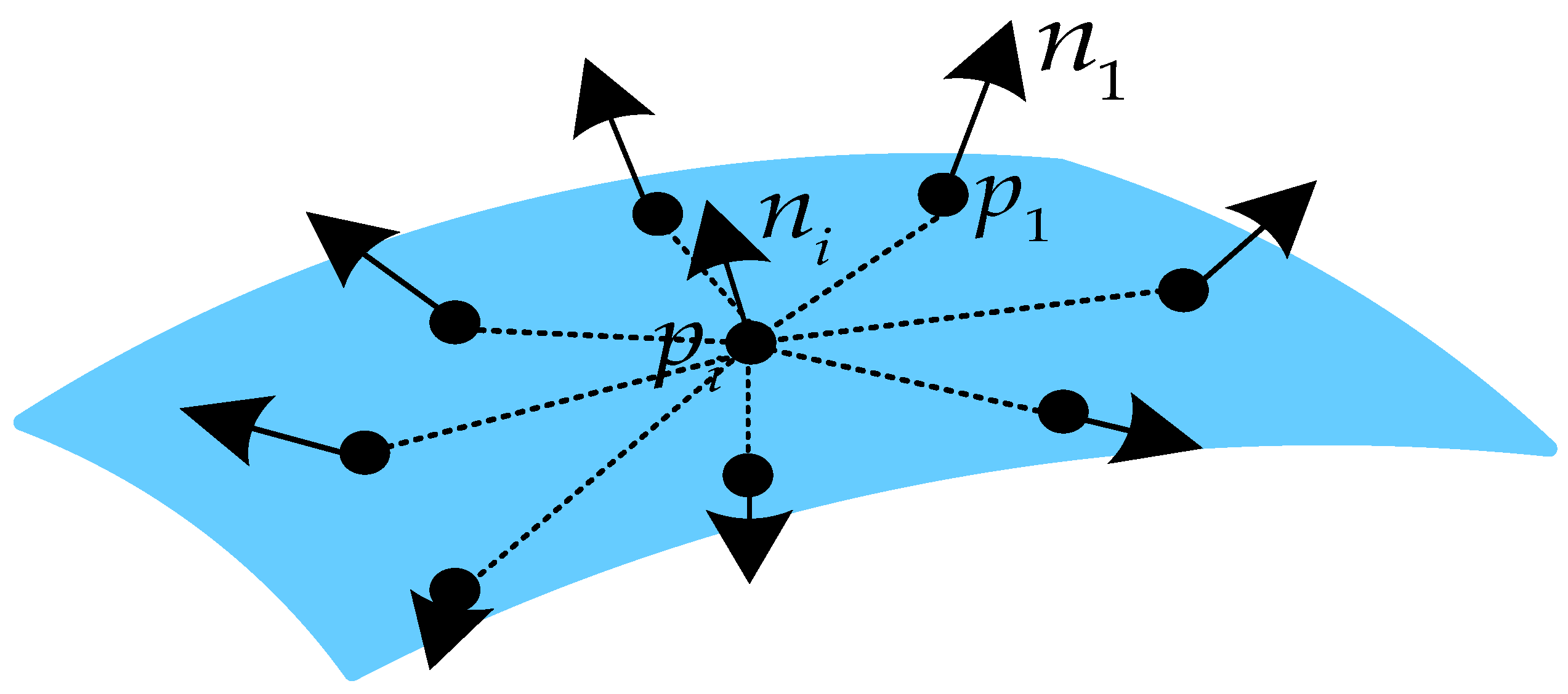
For a pair of points $(p_i,p_j)$ in a local region, in order to describe the geometric relationship between two points, a four-dimensional descriptor is introduced:

$${\psi }_{ij}=(\Vert d\Vert ,\angle (n_i,d),\angle (n_j,d),\angle (n_i,n_j))$$

(3)

where d is the vector, which represents the difference between two points in the feature space, and $\Vert ·\Vert$ is the Euclidean distance. $n_i$ and $n_j$ are the normal vectors of $p_i$ and $p_j$ in the local region, respectively. As shown in Equation (4), $\angle$ is the angle between two normal vectors.

$$\angle (n_i,n_j)=a\tan 2(\Vert n_i\times n_j\Vert ,n_i·n_j)$$

(4)

The four-dimensional descriptor describes the spatial geometric characteristics of the points pair. For all points $\{p_1,p_2,p_3,\dots ,p_j\}$ in a local region, with $p_i$ as the center and k as the radius (k is 0.4 in our method), we contain j point pairs with center point $p_i$. Then, the encoding method of this local region is expressed as Equation (5):

$$F_i=[p_1,n_1,p_2,n_2,\dots ,p_j,n_j,{\psi }_{i1},{\psi }_{i2}\dots ,{\psi }_{ij}]$$

(5)

where $n_j$ is the normal vector of point $p_j$, and ${\psi }_{ij}$ is the four-dimensional feature descriptor between point $p_j$ and center point $p_i$. As shown in Figure 2, $F_i$ describes the spatial geometric characteristics of the local region via the local feature descriptor between all points with center point $p_i$ in this local region.

3.3. Pose Prediction Network

In this section, we utilize the PointNet with the local feature descriptor to construct a prediction network for head pose estimations; the structure of the head pose prediction network is shown in Figure 3.

As shown in Figure 3, for an input object with 4096 points $\{p_1,p_2,p_3,\cdots ,p_{4096}\}$, we select every point as the center of a sphere with radius k (k is 0.4 in our method), and the points in the same sphere are regarded as being in the same local region $\{L_1,L_2,L_3,\cdots ,L_{4096}\}$. For each $L_i$, we adopt the local feature descriptor to describe the geometric characteristics of the local region: $\{{\psi }_1,{\psi }_2,{\psi }_3,\cdots ,{\psi }_{4096}\}$ (${\psi }_i$ represents a local geometric characteristic of local region $L_i$). Then, PointNet, as shown in Figure 1, is utilized to extract the features of each ${\psi }_i$. After the above steps, we obtain a set of local features in high-dimensional feature space $\{f_1,f_2,f_3,\cdots ,f_{4096}\}$. Subsequently, a Max pooling layer is used to extract the entirety of feature $F_w$ of all the local features $\{f_1,f_2,f_3,\cdots ,f_{4096}\}$. Finally, three fully connected layers with 256, 64, and 3 filters are adopted to map head feature $F_w$ to three pose angles.

The loss function of our head pose prediction network is defined as follows:

$$L_{predict}={\displaystyle \sum _j^n{\Vert G_j-P_j\Vert }_2^2}$$

(6)

where $G_i$ represents the ground truth of three pose angles (expressed in Euler angles: roll, pitch, and yaw), and $P_i$ is the prediction value of our head pose prediction network.

3.4. Siamese Network for Pose Constraint

As described above, a regression network is constructed to predict head poses, but due to the non-stationary characteristic of the head pose change process, it is difficult for a single regression network to cope with large-scale synthetic training data [23], which will result in a large prediction error. In order to deal with the above problem, a Siamese network with similar samples was proposed to constrain the prediction values and guide the regression process of the pose prediction network.

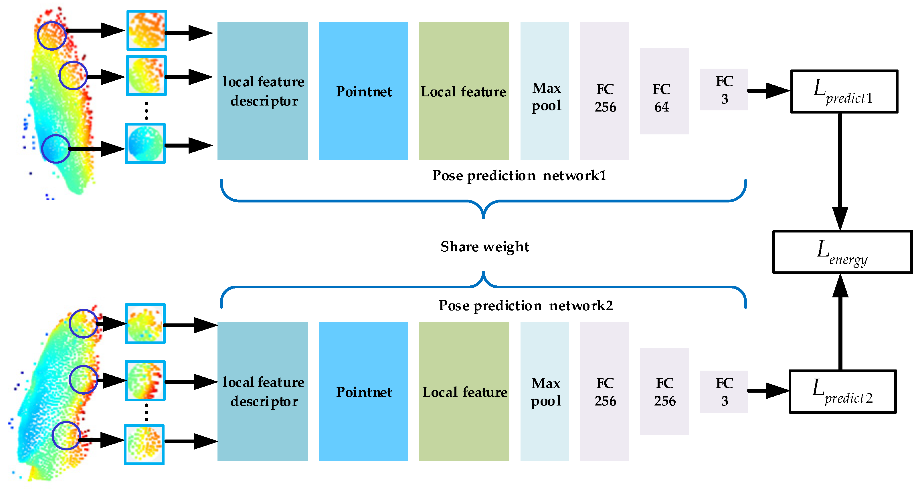
The structure of the proposed Siamese network is shown in Figure 4. The network consists of two identical branches, which accept similar pose samples as the inputs and extract features. The ends of the two branches are connected by an energy function to compute the difference between the two features:

$$L_{energy}={\displaystyle \sum {}_j{}^n\Vert D_{net}(x_i)-D_{gt}(x_i)\Vert {}_2^2}$$

(7)

$$D_{net}(x_j)=P_{1j}-P_{2j}$$

(8)

$$D_{gt}(x_j)=G_{1j}-G_{2j}$$

(9)

where $D_{net}$ is the difference between the two predicted pose angles extracted by their own branch, and $D_{gt}$ represents the difference in their ground truth [38].

Considering that the training dataset has a total of N samples, a large number of N/2 possible pairs can be used, and for a specific pair of samples $(S_i,S_j)$, only those with at least $\gamma$ degrees of the total difference between all the pose angles (ground truth value) are selected:

$$\left|G_{s_i}-G_{s_j}\right|<\gamma$$

(10)

where $\gamma$ determines the similarity of the pair of samples. In the training process, the energy function $L_{energy}$ is also regarded as the loss function of the Siamese network.

Compared with a single-branch network, the proposed Siamese network has two main advantages. First, the parameters between the identical networks are shared, which can guarantee that a pair of very similar samples is not mapped to very different locations in a feature space by the respective networks. Second, as the loss function ($L_{energy}$) converges during training, similar pose samples within $\gamma$ are extracted by their own network, which enables two regression networks to supervise each other and prevents the other side from being mapped to a more distant area in the feature space. In the testing stage, we only employ one pose prediction network to estimate the head pose (the parameters of the two networks are tied).

The hyperparameters of our Siamese network are as follows: the learning rate is 0.001, the decay rate is 0.99, the batch size is 64, and the decay step size is 500.

4. Experiments

In this section, we first introduce two public datasets for experiments: the Biwi Kinect Head Pose dataset and Pandora. Second, in order to verify the effect of the local feature descriptor and investigate similarity $\gamma$ in Equation (10), we conduct ablation experiments on the Biwi Kinect Head Pose dataset. Third, we investigate the influence of the input number of points. Finally, we use our best results for comparison experiments with the latest methods and analyze the results.

4.1. Datasets

With respect to the Biwi Kinect Head Pose dataset, Fanelli et al. [39] utilized Kinect to collect this dataset. This dataset has a total of more than 15,000 head pose images, each object contains depth maps and the corresponding RGB images, and the resolution is $640\times 480$. Biwi records 24 sequences of 20 different objects (6 females and 14 males, some of them are recorded twice). It is a challenging dataset with various head poses and partial occlusion. The test set includes sequences 11 and 12, which contain around 1304 images, and the training set contains the remaining 22 sequences, which contain around 14,000 images.

With respect to the Pandora dataset, Borghi et al. [1] collected this dataset specifically for head and shoulder pose estimations. Pandora has a total of more than 250,000 images, and each object contains depth maps (the resolution is $512\times 424$) and corresponding RGB images (the resolution is $1920\times 1080$). The dataset records 110 sequences of 10 male and 12 female objects. The recorded objects belonging to the upper body contain various postures, hairstyles, glasses, scarf, etc.

The above two datasets only provide RGB and depth images. We should transform depth images to point clouds before sending them into the Siamese network. First, we directly use the ground truth of the head center $H_c$ with its depth value $D_c$ to obtain the head areas (head detection is not the focus of our method), and we remove the background: we set the depth value as greater than $D_c+300$ to 0 (300 is the general amount of space for a real head and expressed in mm). Second, we transform the depth map from an image coordinate system to a world coordinate system.

$$\left[\begin{array}{c}x\\ y\\ z\end{array}\right]=D_c\left[\begin{array}{ccc}\frac{1}{f_x}& 0& 0\\ 0& \frac{1}{f_y}& 0\\ 0& 0& 1\end{array}\right]\left[\begin{array}{c}{x}^i\\ y^i\\ 1\end{array}\right]$$

(11)

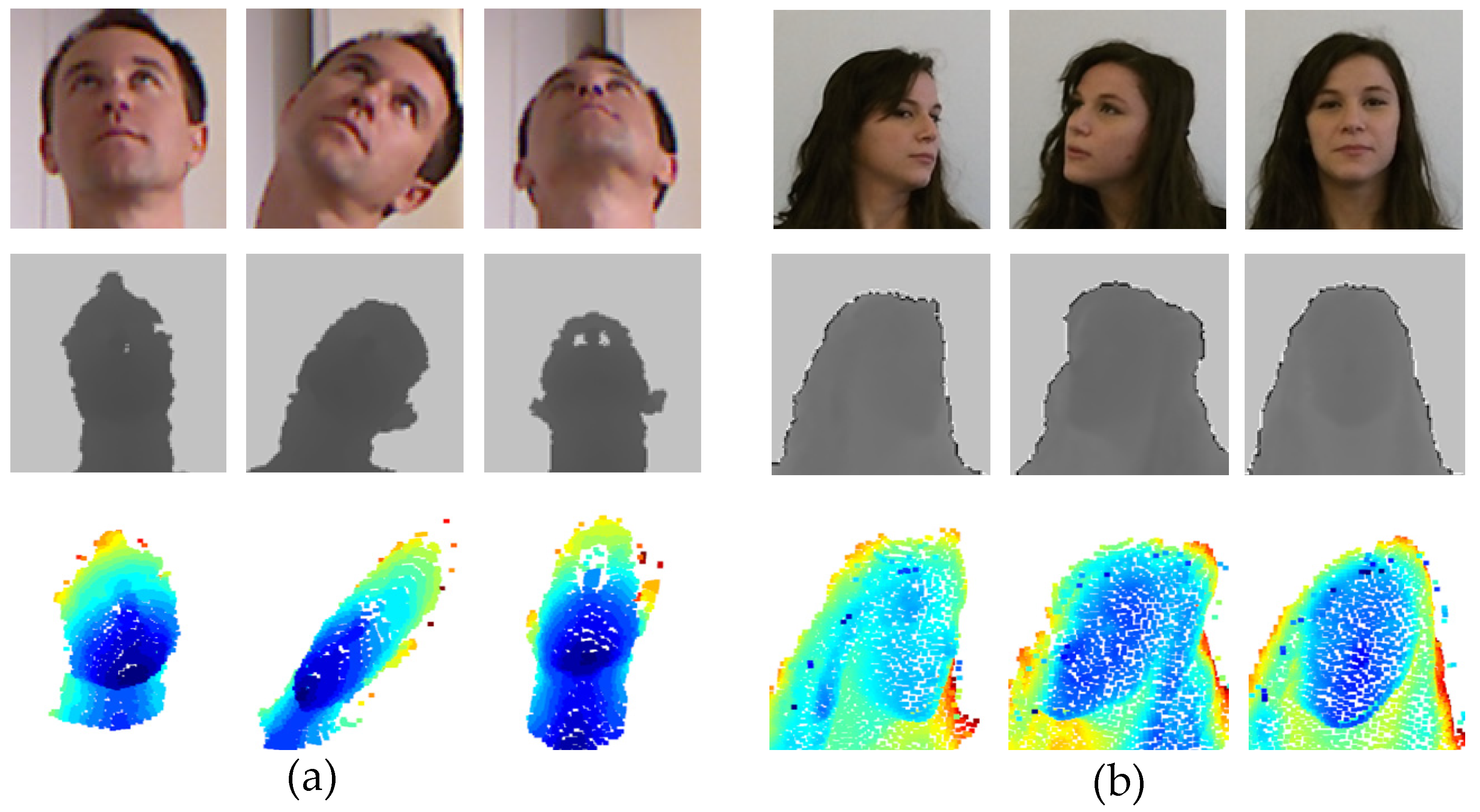
$(x^i,y^i)$ denotes the pixel in the image coordinate system, and $f_x$ and $f_y$ represent the horizontal and vertical focal length of the internal parameters of the depth sensors. $(x,y,z)$ is the position of the point converted from the pixel. Figure 5 shows examples of RGB images, depth maps, and point clouds from the Biwi Kinect Head Pose and Pandora datasets.

Both Biwi Kinect Head Pose and Pandora datasets provide ground truth pose angles (roll, pitch, and yaw). In our experiments, according to previous methods [1,2,23,26,38], we use the mean of the absolute values and the standard deviation to quantitatively evaluate the accuracy:

$$S=\delta \pm \beta$$

(12)

$\delta$ denotes the mean of the absolute values (MAE) of the difference between all ground truth and predicted values, and $\beta$ is the standard deviation of the absolute values (SD) of the difference between all ground truth and predicted values.

4.2. Ablation Experiments

As described in Section 3.2, we introduced a local feature descriptor to describe the local region. In order to verify the effect of our method, according to the method in [7], we replace the local feature descriptor and only use the position information of the points to describe the local region.

In this section, to intuitively demonstrate the effect of the descriptor, we only use a single branch, as shown in Figure 3, to conduct the ablation experiment. The results are reported in

Table 1. Performance evaluation with different local region expressions on the Biwi Kinect Head Pose dataset.

Local Region	Position	Local Feature Descriptor
Roll	$2.2\pm 2.6$	$1.7\pm 2.0$
Pitch	$2.4\pm 2.1$	$2.0\pm 2.2$
Yaw	$2.4\pm 2.2$	$2.4\pm 2.1$
Avg	$2.3\pm 2.3$	$2.0\pm 2.1$
fps	385	288

.

As shown in Table 1, the accuracy of the head pose prediction network greatly improved with the local feature descriptor, where the MAE is reduced by 0.3 and the SD is reduced by 0.2. This is because the descriptor provides the network with detailed local geometric features, which are more conducive to the extraction of the pose characteristics. On the other hand, our method would lead to extra computational costs, but it still maintains a good real-time performance. The results in Table 1 prove the effectiveness of the proposed local feature descriptor.

According to Equation (10) in Section 3.4, $\gamma$ represents the similarity of the pair of samples. For a deep learning network, training samples are a key factor for the performance. In this step, we conduct comparison experiments on Biwi to decide the best $\gamma$ for the Siamese network; the results are reported in

Table 2. Performance evaluation with different $\gamma$ on the Biwi Kinect Head Pose dataset.

$\mathit{\gamma }$	Roll	Pitch	Yaw	Avg
0	$1.7\pm 2.0$	$2.0\pm 2.2$	$2.4\pm 2.1$	$2.0\pm 2.1$
5	$1.7\pm 2.0$	$1.9\pm 2.1$	$2.2\pm 2.1$	$2.0\pm 2.1$
10	$1.5\pm 1.9$	$1.7\pm 2.0$	$2.2\pm 1.9$	$1.8\pm 1.9$
15	$1.3\pm 1.7$	$1.5\pm 1.8$	$2.2\pm 1.7$	$1.6\pm 1.7$
20	$1.3\pm 1.7$	$1.6\pm 1.8$	$2.3\pm 1.8$	$1.7\pm 1.8$
25	$1.4\pm 1.7$	$1.7\pm 2.0$	$2.3\pm 1.8$	$1.8\pm 1.8$
30	$1.5\pm 1.8$	$1.8\pm 2.0$	$2.4\pm 1.9$	$1.9\pm 1.9$
35	$1.6\pm 1.9$	$1.9\pm 2.2$	$2.4\pm 2.1$	$2.0\pm 2.0$
40	$1.9\pm 2.2$	$2.2\pm 2.3$	$2.4\pm 2.2$	$2.2\pm 2.2$
45	$2.3\pm 2.4$	$2.4\pm 2.5$	$2.5\pm 2.3$	$2.4\pm 2.4$
50	$2.5\pm 2.8$	$2.6\pm 2.7$	$2.5\pm 2.5$	$2.5\pm 2.7$

.

As shown in Table 2, when $\gamma =0$, the inputted pair of samples has the same pose angles (same sample), and when the loss function is $L_{energy}=0$, the constraint of the Siamese network is not utilized. As $\gamma$ increases, the two branches of the Siamese network start to constrain each other. When $\gamma =15$, our network achieves the best results. As $\gamma$ continues to increase, the accuracy begins to decline. This is because obtaining more similar pose samples is more conducive to constraining pose angles within a smaller range. However, when $\gamma$ is too small, the Siamese network also cannot achieve the best results because the pose features of the samples are too close, which makes it difficult for the Siamese network to distinguish the difference.

Figure 6 shows the prediction accuracy with different $\theta$ metrics. For each pose angle, if the absolute value of the difference between the prediction value and the ground truth is less than $\theta$, the pose angle is regarded as accurately predicted. According to Figure 6, when $\theta$ is too small, the accuracy is obviously low. When the total difference, $\gamma$, is 5 and 10, the difference in the head pose is quite small, especially for a certain angle.

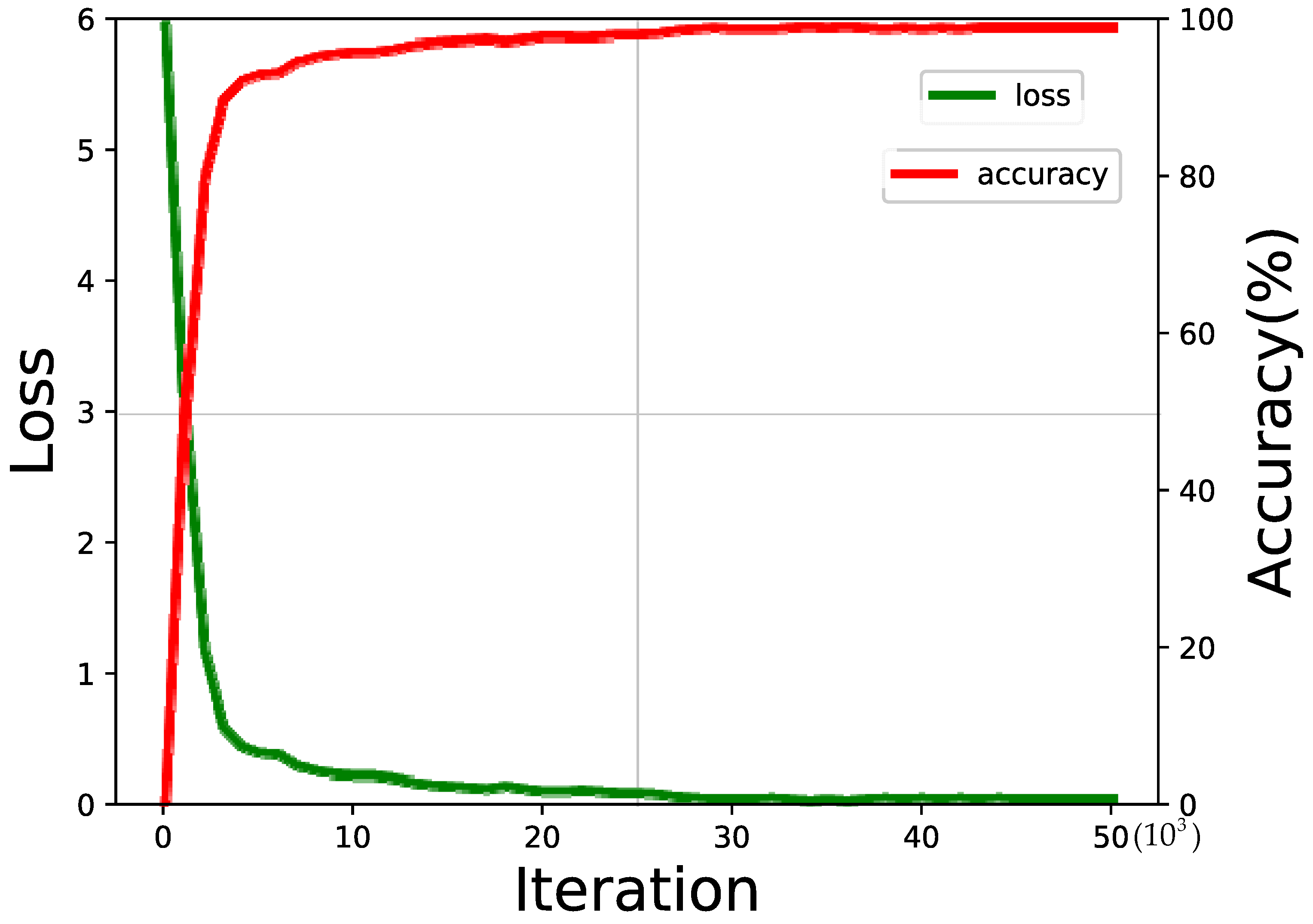
According to Table 2, we set $\gamma =15$ as our best result for comparison experiments. Figure 7 shows the curves of the loss function and the accuracy of the Siamese network during training when $\gamma =15$.

4.3. Input Number of Points

As mentioned above, we sampled 4096 points for each object, but the number of input points affects the performance of the network. As shown in Figure 8, this is because the number of points affects the detailed information of the object and also determines the number of local regions. In this section, we investigate the input number of the points by losing half points for each step (we also adopt the farthest point sampling method to the sample points). The results are reported in

Table 3. Results of the different input numbers of points on the Biwi Kinect Head Pose dataset.

Input Number	Acc	fps
4096	$1.6\pm 1.7$	288
2048	$1.7\pm 1.9$	398
1024	$2.0\pm 2.2$	558

.

As reported in Table 3, our network has a higher accuracy when there is an increased input number of points, which indicates that more points are beneficial for describing the more detailed features of the object and can significantly improve the accuracy of the network, but time consumption increases. However, 4096 points with 288 fps also maintained a good real-time performance for most applications.

4.4. Comparison Experiments

In this section, we conduct comparison experiments on two public datasets, and we analyze the results.

Table 4. Comparison of results achieved by different methods on the Biwi Kinect Head Pose dataset.

Methods	Input	Roll	Pitch	Yaw	Avg
Venturelli et al. [38]	Depth	$2.1\pm 2.2$	$2.3\pm 2.7$	$2.8\pm 3.3$	$2.4\pm 2.7$
Borghi et al. [1]	Depth	$1.8\pm 1.8$	$1.6\pm 1.7$	$1.7\pm 1.5$	$1.7\pm 1.7$
Xiao et al. [2]	Point cloud	$1.5\pm 1.4$	$2.3\pm 1.7$	$2.4\pm 1.8$	$2.1\pm 1.6$
Huang et al. [13]	RGB	3.1	5.2	4.6	4.3
Ma et al. [26]	Point cloud	$1.4\pm 2.0$	$1.5\pm 2.3$	$1.5\pm 2.1$	$1.5\pm 2.1$
Cao et al. [16]	RGB	4.1	4.8	3.0	4.0
Liu et al. [18]	RGB	2.6	4.7	3.4	3.6
Ours	Point cloud	$1.3\pm 1.7$	$1.5\pm 1.8$	$2.2\pm 1.7$	$1.6\pm 1.7$

reports the comparison of the results with the latest methods on the Biwi Kinect Head Pose dataset.

Table 4 lists a comparison of the experimental results on the Biwi Kinect Head Pose dataset. The methods in [13,16,18] only report their MAE, and other methods report $MAE\pm SD$. As shown in Table 4, the accuracy of the depth and point cloud methods is obviously higher than the RGB methods. This is because geometric information is more conducive to the extraction of the pose features, especially under partial occlusion and large pose interferences. Compared with depth maps, point clouds have more abundant geometric information and clearer contours, which are more beneficial to pose feature extraction. Although Borghi et al. [1] achieved a very high accuracy and only relied on depth maps, they used two Gan networks to generate gray and motion images, which leveraged three types of images to jointly predict the head pose, and the entire network structure is too complex.

As per the results reported in Table 4, compared with the methods in [1], our MAE was reduced by 0.1, and compared with the methods in [26], although their MAE is lower, our SD was reduced by 0.4. Overall, the accuracy of our method is higher than that of the other methods.

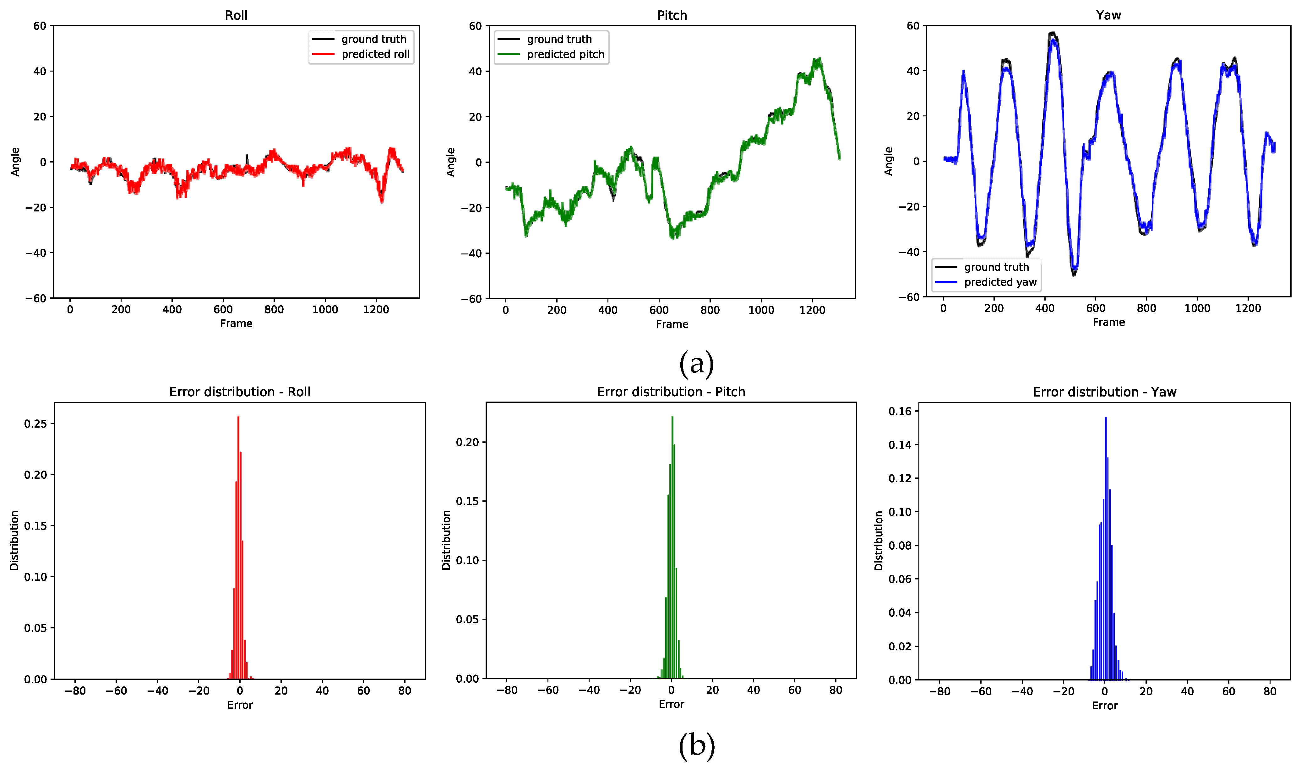
In order to intuitively show the test results on the Biwi Kinect Head Pose dataset, Figure 9a shows the ground truth and the prediction values of all the test samples, and Figure 9b shows the error distributions for each pose angle. As shown in Figure 9, the prediction results are very close to the ground truth, and the error distribution is convergent.

Table 5. Comparison of results achieved by different methods on the Pandora dataset.

Methods	Input	Roll	Pitch	Yaw	Avg
Borghi et al. [1]	Depth	$5.4\pm 5.1$	$6.5\pm 6.6$	$10.4\pm 11.8$	$7.4\pm 7.8$
Xiao et al. [23]	Point cloud	$4.3\pm 4.5$	$6.1\pm 5.6$	$8.6\pm 9.8$	$6.3\pm 6.6$
Ma et al. [26]	Point cloud	$4.9\pm 7.4$	$6.4\pm 10.5$	$9.6\pm 15.3$	$7.0\pm 11.0$
Ours	Point cloud	$4.3\pm 4.7$	$6.0\pm 5.2$	$8.3\pm 9.8$	$6.2\pm 6.6$

lists a comparison of the experimental results on the Pandora dataset, which contains more abundant samples with a series of large body gestures and partial occlusion. As reported in Table 5, our accuracy outperforms the latest methods. Compared with Xiao et al. [23], our accuracy is very close to theirs, and only the MAE was reduced by 0.1, but for each pose angle, our MAE and SD were better than theirs, except for the SD of the roll angle. 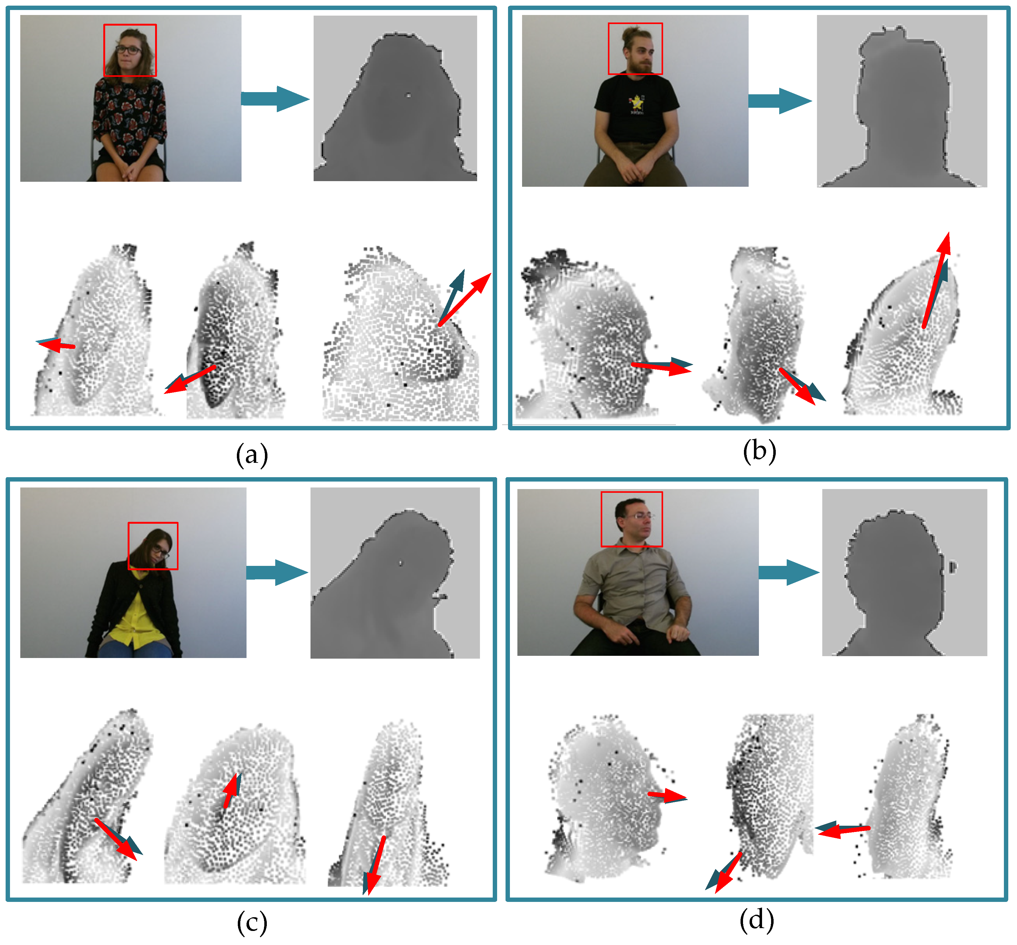Figure 10 shows the examples of our method on Pandora.

As shown in Figure 10, our method can cope well with pose predictions with respect to various pose changes and provide an accurate pose angle estimation.

For the head pose estimation task, except for the accuracy, the time cost is also an important indicator for measuring performance, which determines whether the method can be applied to real application scenarios.

Table 6. Comparison of different methods in terms of time costs.

Methods	fms
Xiao et al., 2020 [2]	125
Xiao et al., 2020 [23]	117
Wang et al., 2022 [21]	148
Wang et al., 2023 [5]	225
Ours	288

lists a comparison of different methods in terms of time costs. Because different data types are processed in different ways, for a fair comparison, we only conducted comparisons with point cloud methods.

As shown in Table 6, compared with recent head feature extraction methods, our method is faster. This is because the local feature descriptor described the spatial geometric features of the local regions in detail before the deep learning network, which allows us to adopt a shallow network to extract the features and enables the network to maintain a good real-time performance.

Combining Table 4 and Table 5, it is noticeable that our accuracy outperforms the latest methods, and Table 6 proves that our network also has a good real-time performance.

We conducted our experiments on the following operating system: Ubuntu16.04. The used hardware is listed as follows: the GPU is NVIDIA GTX1080ti, the CPU is Intel Core i7 (3.40 GHz), the display is SAMSUNG S27R350FHC (75 Hz, resolution: $1920\times 1080$), and the depth cameras are Kinect v2 (resolution: $640\times 480$) for the Biwi Kinect Head Pose dataset and the Kinect one (resolution: $512\times 424$) for the Pandora dataset.

5. Conclusions

In this study, in order to cope with the non-stationary characteristic of the head pose change process, a new Siamese network with a local feature descriptor was constructed for 3D head pose estimations. In the feature extraction stage, a four-dimensional descriptor is introduced to describe the geometrical relationship between a pair of points, which can describe the geometric characteristics of the local regions in detail. In the head pose estimation stage, similar pose samples were used to constrain the regression process of the pose angles. Ablation experiments proved the effectiveness of the local feature descriptor, and the results of the experiments on public datasets show that compared with the latest methods, our accuracy outperformed the other methods (where SD was reduced by 0.4 and MAE was reduced by 0.1). Simultaneously, the proposed method also maintained real-time performance and can be applied to real application scenarios. However, in the case of partial occlusions, the accuracy is still not sufficient. In future studies, we will further explore algorithms and optimize the network and explore new methods for other 3D face analysis technologies.